


Abstract
The  state of the hydrogen molecule has the second largest triplet-state excitation cross-section, and plays an important role in the heating of the upper thermospheres of outer planets by electron excitation. Precise energies of the H2, D2, and HD
  (
( ) levels are calculated from highly accurate ab initio potential energy curves that include relativistic, radiative, and empirical non-adiabatic corrections. The emission yields are determined from predissociation rates and refined radiative transition probabilities. The excitation function and excitation cross-section of the
  state are extracted from previous theoretical calculations and experimental measurements. The emission cross-section is determined from the calculated emission yield and the extracted excitation cross-section. The kinetic energy (Ek) distributions of H atoms produced via the predissociation of the
  state, the
  –
–  dissociative emission by the magnetic dipole and electric quadrupole, and the
  –
–  –
–  cascade dissociative emission by the electric dipole are obtained. The predissociation of the
  and
and  states both produce H(1s) atoms with an average Ek of ∼4.1 eV/atom, while the
  –
–  dissociative emissions by the magnetic dipole and electric quadrupole give an average Ek of ∼1.0 and ∼0.8 eV/atom, respectively. The
  –
–  –
–  cascade and dissociative emission gives an average Ek of ∼1.3 eV/atom. On average, each H2 excited to the
  state in an H2-dominated atmosphere deposits ∼7.1 eV into the atmosphere while each H2 directly excited to the
  and
and  states contribute ∼2.3 and ∼3.3 eV, respectively, to the atmosphere. The spectral distribution of the calculated continuum emission arising from the
  –
–  excitation is significantly different from that of direct
  or
or  excitations.
Export citation and abstract BibTeX RIS
1. Introduction
The electron impact excitation of H2 from the  state to the triplet states takes place via electron exchange processes and has very large cross-sections in the threshold energy region. All triplet excitations, in the absence of collisional deactivation, are dissociative. Therefore, their excitation by low-energy electrons is a very efficient breakup mechanism of H2. Furthermore, the lowest triplet state,
  , is strongly repulsive and the dissociation, predissociation, and dissociative emission of the triplet states, one way or another, are usually due to the
  state. Therefore, the H atoms produced from the breakup process are also often kinetically hot. Although H2 can be excited to the singlet-ungerade states by both photons and electrons, both dissociation and predissociation ultimately take place via the continuum levels of bound states (Liu et al. 2010b). Moreover, the great majority of H2 molecules excited to the singlet-ungerade states return to the discrete levels of the
  state by photoemission. The dissociation and predissociation of the singlet-ungerade states not only have small cross-sections, especially at low impact energies, but also produce slow H atoms (Liu et al. 2009, 2010b, 2012). For these reasons, the triplet excitation is the most efficient breakup channel of H2 in converting the excessive electronic energy into the kinetic energy (Ek) of the outgoing H atoms (Liu et al. 2010a, 2016).
In the upper part of the atmospheres of H2 gas giants, the presence of a large number of low-energy electrons efficiently produces a large number of fast-moving H atoms by triplet excitation and dissociation. The collision of these hot H atoms with H2 and other atmospheric species distributes the heat to other parts of the atmosphere. For this reason, the triplet excitation of H2 by low-energy electrons is a very important mechanism of the energy deposition in H2-dominated atmospheres (Shemansky et al. 2009). The physical parameters for the triplet excitation and dissociation rates, and the kinetic energy distribution of H atoms produced from triplet excitation are required to model the energy deposition rate by electrons.
The  state is the second ungerade state and the second lowest triplet state after the
  state. The
  state also has the second largest triplet excitation cross-section after the
  state. The
  cross-sections measured with electron energy loss (EEL) by Wrkich et al. (2002) are a factor of 2.5 and 4.3 greater than the corresponding
  cross-sections at 20 and 30 eV, respectively. The more recent EEL measurement of Hargreaves et al. (2017) likewise shows that the
  cross-section is a factor of 2.3−2.9 greater than the
  counterpart in the energy region of 14 to 17.5 eV. Unlike excitation to the
  state, which results in 100% direct dissociation and fully converts the excess electronic energy into kinetic energy, the dissociation of H2 in the
  state, depending on the orbital symmetry, takes place via different mechanisms. The
  state is rapidly predissociated within a fraction of a nanosecond by electronic Coriolis coupling with the
  state (de Bruijn et al. 1984; Martín & Borondo 1988). The
  state, however, can only be weakly predissociated by the spin–orbit and spin–spin interactions with the
  state (Chiu & Bhattacharyya 1979; Liu et al. 2017). Consequently, the spontaneous emissions of the
  state by the electric dipole (E1), magnetic dipole (M1), and electric quadrupole (E2) moments are competitive processes (Chiu & Lafleur 1988). The excess electronic energy is fully converted to the Ek of the outgoing H atoms in a predissociation process, whereas it is only partially converted into the Ek of the outgoing H atoms in a dissociative emission process.
The  −
−  and
and  −
−  transition probabilities, and the predissociation rates of the
  state, along with the
  energy levels, were obtained in the recent work of Liu et al. (2017). Those rates have produced calculated lifetimes that are in good agreement with the experimental measurement of the
  (v = 0) levels of H2, HD, and D2, obtained by Johnson (1972), and the other
  levels of H2, obtained by Berg & Ottinger (1994). In the present work, those quantities are further refined by using more accurate potential energy curves and by including an empirical non-adiabatic correction to the bound state. An
  −
−  excitation function is also extracted from the theoretical calculation of Lee et al. (1996). The shape of the derived excitation function agrees well with that of the EEL cross-section of Khakoo & Trajmar (1986) over the entire (20−60 eV) measured range and with that of the
  time-of-flight (TOF) measurement of Ottinger & Rox (1991) from threshold energy to 22 eV. The Ek distributions of the
  and
and  predissociation process and of the
  −
−  and
and  −
−  −
−  dissociative emission, along with the branching ratios of various decay channels, are obtained over a wide range of excitation energies. The present work is the third paper on the kinetic energy distribution of H atoms produced from electron impact H2 triplet excitations. Our earlier work on the distributions from direct excitation to the
  and
and  states have been reported in Liu et al. (2010a) and Liu et al. (2016), respectively.
Some rotational levels of the  state are metastable, which means that radiative emission by electric dipole to a lower state is impossible. It arises from the fact that the rotational levels (N) of the v = 0 state and, possibly, a few very high N levels of the v = 1 state of the
  state fall below their counterparts in the v = 0 state of the
  electronic state. The
  state appears to be the only metastable state of H2 (and its isotopologues). The long lifetime of the
  state makes it an ideal species for experimental investigations of higher triplet states (Helm et al. 1984; de Bruijin & Helm 1986; Jozefowski et al. 1992, 1994a, 1994b; Sprecher et al. 2013). The
  metastable species is usually prepared either with the reaction of
  with alkaline metal vapor (de Bruijn et al. 1984; Lembo et al. 1988, 1990; Koot et al. 1989a, 1989b; Siebbeles et al. 1992; Wouters et al. 1996, 1997) or with the low-energy electron excitation of H2 (Lichten & Wik 1978; Eyler & Pipkin 1981; Ottinger & Rox 1991; Kim & Mazur 1995). Many theoretical calculations of the predissociation (Chiu 1965; Chiu & Bhattacharyya 1979; LaFleur & Chiu 1986; Liu et al. 2017) and radiative decay (Bahattacharyya & Chiu 1979; Chiu & Lafleur 1988) rates of the
  state have been performed in an attempt to reproduce the
  experimental lifetimes of Johnson (1972) and Berg & Ottinger (1994).
Direct photoexcitation from the  state to a triplet state of H2 is strongly forbidden because of very weak electron spin–orbit interaction. Nevertheless, Jungen & Glass-Maujean (2016) recently suggested an indirect mechanism by which triplet states can be populated with a single photon excitation from the
  state. They identified lines from photoexcitation of nf singlet-ungerade Rydberg levels from the
  state, which take place by intensity borrowing through the p–f interaction. Since the singlet and triplet nf Rydberg series can be readily mixed through hyperfine interaction, their observation suggested that the radiative decay of the nf levels and the subsequent cascade can lead to a population at the metastable
  level and other triplet levels.
The structure of H2 triplet states has been investigated extensively using various experimental methods. Dieke and co-workers carried out extensive discharge emission studies with a spectrometer and photographic plates. The results of those investigations were summarized as extensive H2 wavelength tables of Dieke by Crosswhite (1972). Experimental techniques such as electron-induced microwave optical magnetic resonance (Freund & Miller 1973; Miller et al. 1974) and electron–photon or photon–photon delayed coincidence (Mohamed & King 1979; Kiyoshima et al. 1999, 2003) were also utilized to investigate the triplet states. High-resolution laser spectroscopy (Lichten et al. 1979; Eyler & Pipkin 1981; Jozefowski et al. 1992, 1994a, 1994b; Berg & Ottinger 1994; Ottinger et al. 1994; Siebbeles et al. 1996; Sprecher et al. 2013) has also been widely used. Extensive investigations of the dissociation dynamics of the n ≥ 3 triplet Rydberg series have been carried out with  −Cs fast-beam photofragment spectroscopy (de Bruijin & Helm 1986; Bjerre et al. 1988; Lembo et al. 1988, 1990; Koot et al. 1989a; Schins et al. 1991; Siebbeles et al. 1992; Wouters et al. 1996, 1997). Other techniques such as Fourier-transform infrared spectroscopy (Herzberg & Jungen 1982; Jungen et al. 1989, 1990; Bailly & Vervloet 2007) and infrared laser spectroscopy (Dabrowski & Herzberg 1984; Davies et al. 1988, 1990a, 1990b; Uy et al. 2000) have also been employed to study the Rydberg transitions of triplet states.
Unlike the singlet-ungerade states, where the investigations of classical discharge emission spectroscopy (Herzberg & Jungen 1972; Dabrowski 1984; Abgrall et al. 1993a, 1993b, 1993c, 1994; Roncin & Launay 1994) have helped to determine the energies of over 85% of the discrete levels of the first four electronic states, the experimentally determined energy levels of the triplet states are very limited. Even for the two lowest bound triplet states,  and
and  , less than 10% of the energy levels have been experimentally determined. This is primarily caused by much smaller transition probabilities and branching ratios than their counterparts in singlet-ungerade states. As direct photoexcitation from the
  ground state to a triplet state is strongly forbidden, the investigation of triplet states with laser spectroscopy typically requires preparation of metastable H2 by either electron impact excitation from the
  (0) level or reaction of
  with alkaline metal vapor. The similarity of the triplet potential curves limits the range of vibrational levels of the other triplet states that can be accessed from the low v levels of the
  state. One of the goals of the present paper is to provide accurate calculated energies of the
  state that can help future experimental analysis.
All measurements of the absolute excitation cross-section of the  state have so far been carried out with EEL spectroscopy. Khakoo & Trajmar (1986) measured the absolute cross-section at 20, 30, 40, and 60 eV, while Wrkich et al. (2002) reported corresponding values at 17.5, 20, and 30 eV. The difference between the two sets of EEL cross-sections at 20 and 30 eV are greater than their joint error limits. Hargreaves et al. (2017) recently reported EEL measurement of the
  state at 14, 15, 16, and 17.5 eV. Mason & Newell (1986) measured relative excitation functions of the
  metastable species with a TOF technique, while Ottinger & Rox (1991) measured the excitation function with both TOF and laser-induced fluorescence (LIF) techniques. Harries et al. (2004) also obtained the relative excitation function by laser excitation of the metastable H2 to higher Rydberg states followed by a field ionization. Furlong & Newell (1995) investigated the resonant excitation of the
  state. Lee et al. (1993, 1996) calculated the excitation cross-sections in single
  ro-vibronic levels. Lima et al. (1988), da Costa et al. (2005), and Taveira et al. (2006) also computed the cross-sections of
  and other triplet states. More recently, Zammit et al. (2017) obtained the excitation cross-sections of the
  state and other singlet and triplet states over a wide range of excitation energies with more accurate convergent-close-coupling (CCC) calculations. Finally, Laricchiuta et al. (2004) calculated the cross-sections for excitations between several pairs of triplet states.
The triplet states of H2 have been the subject of many theoretical calculations. Depending on the relative velocity of the Rydberg electron and nuclei, two primary theoretical methods are used. For the low n Rydberg state, the Rydberg electron moves much faster than the nuclei. Traditional ab initio calculations are often used. These calculations attempt to obtain accurate Born–Oppenheimer (BO) potentials, adiabatic corrections, electronic transition dipole matrix elements, and occasionally, non-adiabatic coupling matrix elements. The theoretical works of Bishop & Cheung (1981), Kolos & Rychlewski (1977, 1990a, 1990b, 1994, 1995), Orlikowski et al. (1999), Staszewska & Wolniewicz (1999, 2001), Wolniewicz (2007), and Corongiu & Clementi (2009) are instances of traditional ab initio calculations of triplet states. The calculation usually deals with a few isolated low n states, although Wolniewicz et al. (2006) calculated the non-adiabatic coupling matrix elements of the first six  and first four
  states, along with their potential energy curves and the dipole transition moments from the
  state (Wolniewicz & Staszewska 2003a, 2003b). However, as n increases, the excited Rydberg electron gets farther away from the ion core. The velocity difference between the Rydberg electron and nuclei becomes smaller, which renders the traditional adiabatic approximation less appropriate. The other method, multichannel quantum defect theory (MQDT), is employed for the calculation of a large number of (usually close-lying) Rydberg states. MQDT often uses accurate potential energy curves of the low n states obtained from traditional ab initio calculations to extract quantities such as quantum defect (Glass-Maujean & Jungen 2009). When calculating spectral intensities, it also uses the accurate electronic transition moments obtained by the ab initio techniques and extends them to high n Rydberg states. Ross & Jungen (1994), Matzkin et al. (2000), Ross et al. (2001), Kiyoshima et al. (2003), Sprecher et al. (2013, 2014), and Oueslati et al. (2014) have performed a number of MQDT investigations of the triplet structure of H2. Staszewska & Wolniewicz (1999, 2001) have calculated accurate BO potentials and adiabatic corrections of many triplet states as well as the electric dipole transition moments among these states. Fine-structure spin–spin constants for a number of triplet states and transition moments among the triplet states have also been computed by Spielfiedel et al. (2004a, 2004b). The transition probabilities and transition moments for
  and a number of other triplet electronic transitions were also obtained by Guberman & Dalgarno (1992). Finally, Wolniewicz (2007) has calculated accurate energy term values of the
  state by including non-adiabatic correction.
The calculation of the  state is an extreme case of the great success in the application of traditional ab initio methods. The
  energies and nuclear wave functions can be accurately obtained from a single potential energy curve (Pachucki & Komasa 2016), where the effect of the coupling with other states is treated as a small non-adiabatic correction (Wolniewicz 1993, 1995a). Progress made in the past several years on the refinement of the
  state's relativistic (Piszczatowski et al. 2008; Puchalski et al. 2016), radiative (Piszczatowski et al. 2009), adiabatic (Przybytek & Jeziorski 2012; Pachucki & Komasa 2014), and non-adiabatic corrections (Pachucki & Komasa 2015) have helped to reduce the difference between the calculated and measured energies within experimental uncertainties of ∼0.001 cm−1 for low (
 ) levels and ∼0.005 cm−1 for high (
 ) levels (Komasa et al. 2011; Niu et al. 2014, 2015; Tan et al. 2014; Trivikram et al. 2016). However, the difference in the calculated and measured energies for several lowest singlet-ungerade states typically ranges from a few tenths of 1 cm−1 to ∼1.5 cm−1, whether the calculation is by semi-ab initio (Abgrall et al. 1993a, 1993b, 1993c, 1994), coupled Schrödinger equations (Wolniewicz et al. 2006), or MQDT (Glass-Maujean & Jungen 2009; Glass-Maujean et al. 2011a, 2011b, 2013a, 2013b, 2013c). For triplet states, the difference is even larger, ranging from a few tenths of 1 cm−1 to ∼2.5 cm−1 (Ross et al. 2001; Kiyoshima et al. 2003; Wolniewicz 2007; Sprecher et al. 2013, 2014; Oueslati et al. 2014; Liu et al. 2016).
2. Theory
Following the notation of our previous work (Liu et al. 2017), the subscript indices i and j in the present work will be used to denote the appropriate quantum numbers of the  and
and  states. The index k will refer to either the
  or
or  states. Since electron spin interactions of triplet states are generally negligibly small (Lichten et al. 1979; Spielfiedel et al. 2004b), the rotational levels of the
  state is well-described by Hund's case (b) and are labeled by vibrational and rotational quantum numbers (
 ). Consequently, physical parameters such as excitation cross-sections, Franck–Condon factors (FCFs), and spontaneous transition probabilities do not depend on the orientation of the electron spin. However, the predissociation of the
  state, taking place via spin–spin and spin–orbit coupling with the repulsive
  state, depends strongly on the particular fine-structure component of a given (
 ) level (Chiu & Bhattacharyya 1979; Berg & Ottinger 1994; Liu et al. 2017). The three fine-structure components are commonly referred to as the F1, F2, and F3 components, which correspond to J = N + 1, J = N, and J =
  , respectively. Since both J and N must be no less than 1 for the
  state, the F3 component does not exist for the N = 1 level.
2.1. Electron Impact  Excitation

The steady-state volumetric decay rate (I) from continuous electron impact excitation is proportional to the excitation rate and decay branching ratio:

where  is the (
 ) to (
 ) decay rate. In the case of photoemission,
  is the spontaneous transition probability. In the case of predissociation, it is the predissociation rates.
  is the total transition probability that includes both radiative and non-radiative components. The predissociation rate and spontaneous transition probabilities of the
  state used in the present investigation are based on the recent work of Liu et al. (2017), with additional refinements described in Sections 2.2 and 3.2.
The excitation rate,  , to level (
 ) is proportional to the population of molecules in the initial level,
  ), the excitation cross-section (σ), and the electron flux (Fe):

Following the approach of Liu et al. (2003, 2016), the cross-section,  , is given by
where  and
and  are the projections of the total electron orbital angular momentum on the internuclear axis for states i and j, respectively, and (:::) is the Wigner 3j-symbol. It is assumed that the basis function is properly symmetrized so that Λ is non-negative (Lefebvre-Brion & Field 2004).
  measures the relative contribution of the multipolar component to excitation, and the summation of
  over r is unity.
  is the so-called degeneracy factor and is given by

The electronic term,  , of Equation (3) accounts for the magnitude and energy dependence of the electronic band cross-section. The vibrational term,
  , is the rotationally dependent FCF,
  .
.  , which describes the shape of the excitation cross-section, is conveniently represented in a functional form by a set of collision parameters. An appropriate functional form for the spin-forbidden and dipole-allowed excitation such as
  −
−  is (Shemansky et al. 1985a, 1985b)
where Ry and E, both in units of eV, are the Rydberg constant and the electron excitation energy, respectively. X is the dimensionless excitation energy in units of the transition energy (i.e.,  ), and a0 is the Bohr radius. Cm (m = 0−6) are the collision strength parameters, whose absolute values can be determined from a fit of the measured or calculated cross-sections over an appropriate energy range. In the present investigation, the absolute value of C5 and the relative values of Cm/C6 (m = 0−4) are determined from a nonlinear least-squares fit of the cross-sections from Ni = 0 and 2 of the
  (vi = 0) state to Nj = 2 of the vj = 0−3 levels of the
  state calculated by Lee et al. (1996). The absolute value of the C6 term is obtained by normalizing the
  cross-section to the 40 eV EEL cross-section measured by Khakoo & Trajmar (1986).
2.2. Potential Energy Curves
The nuclear wave function and corresponding energy  are calculated by numerically solving the Schrödinger equation. To calculate the vibrational wave functions, energies, and other quantities such as FCFs, predissociation rates, and transition probabilities as accurately as possible, a number of refinements on the potential energy curves used in previous works (Liu et al. 2010a, 2016, 2017) were made. These refinements are described below.
The potential energy curves in the present investigation consist of BO potentials ( ), plus adiabatic (
 ), relativistic (
 , radiative (
 ), and (empirical) non-adiabatic (
 ) corrections:

The  and
and  of the
  ,
,  , and
, and  states are taken from the ab initio calculation of Staszewska & Wolniewicz (1999). The
  of the
  state (up to 20.5 a0) was obtained from the calculations of Wolniewicz (1993), Wolniewicz et al. (1998), and Jamieson et al. (2000). The
  of the
  state, however, was obtained from more accurate calculations of Pachucki & Komasa (2014) and Przybytek & Jeziorski (2012). The relativistic correction,
  , consists of four components, which are usually called the mass–velocity, Breit, and the one- and two-electron Darwin terms (Wolniewicz 1993; Piszczatowski et al. 2009). The two-electron Darwin term declines exponentially at large R. The two-electron Darwin term calculated by Wolniewicz (1993) is used in the present work. Similarly, the one-electron Darwin, Breit, and mass–velocity terms up to R = 10a0 calculated by Wolniewicz (1993) are used. Above 10a0, however, the asymptotic forms of Piszczatowski et al. (2008, 2009) are utilized. For the radiative correction,
  ,
,  , and the one-loop
  obtained by Piszczatowski et al. (2009) are used.
To the authors' knowledge, no relativistic and radiative corrections for the triplet states have been reported. Even for the singlet-ungerade states, the relativistic correction is available only for the  and
and  states (Wolniewicz 1995c; de Lange et al. 2001). For the
  state, Wolniewicz et al. (2006) assumed an R-independent value of 0.308 cm−1 for
  . In previous works (Wolniewicz 2007; Liu et al. 2010a, 2016, 2017), the
  of the triplet states were set to be that of the
 state calculated by Bukowski et al. (1992). The relativistic correction,
  , was obtained as the sum of the relativistic corrections of the
 core and the excited H atom of the separate atomic limit to which the triplet correlates. The former was obtained by Howells & Kennedy (1990) over a wide range of R. The latter, which is R-independent and includes relativistic, spin–orbit, and Darwin corrections, is described in many standard textbooks (e.g., Hertel & Schulz 2015). As noted in Wolniewicz (2007) and Liu et al. (2016), this approach underestimates the energies of some levels of the
  and
and  states by overestimating
  (or underestimating
  ).
).
The present work attempts to obtain more accurate  and
and  by interpolating corresponding quantities of the H2
  state and the
 state. All low-lying triplet states correlate to the H(1s) + H(
 ) dissociation limits at large R. The idea is that as n increases, both
  and
and  approach their respective values in the
 state. Since the asymptotic limit of the
  state is H(1s) + H(1s), its
  and
and  are taken to be identical to those of the
  state.4
For the excited triplet states, the following method was used.5
First, the difference in
state.4
For the excited triplet states, the following method was used.5
First, the difference in  between the H2
  state and the
 state is obtained as Δ
 =
=  , where
  and
and  are the radiative corrections of H2
  and
and 
 , respectively. Then, Δ
 is used to interpolate the correction of the excited triplet states. Since the Lamb shift primarily takes place with the s electron, the radiative correction of a state that correlates with the H(1s) + H(ns) can be obtained as
  =
=  +Δ
+Δ . Since
  is not exactly equal to twice
  ,
,  for the n = 2 and 3 states may be more appropriately obtained by a direct reference to the H(1s) + H(1s) limit of the
  state as
  . The Lamb shifts of H(2
 ) and H(2
 ) are about a factor of 83 smaller than their H(2
 ) counterpart. Moreover, the shifts of the
  and
and  levels are nearly equal in value but with opposite signs (Hertel & Schulz 2015). For this reason, the radiative correction for a state that correlates with H(1s) + H(
 ) with
  can be taken as either
  for n = 2 and 3 or
  for n > 3.
For the interpolation of the relativistic correction, the difference in  is formed as
  =
=  , where Erel(1s) = −1.46092 cm−1 is the relativistic correction of the H(1s) atom. The relativistic correction of a state that correlates with the H(1s) + H(
 ) dissociation limit is then obtained as
  =
=  . For
. For  > 0, a proper average of the Erel of the
  + 1/2 and
  − 1/2 levels is needed.
The dominant electron configuration of the  state is (1
 )(2
)(2 ) in the short R(∼1a0) region and
  in the asymptotic region. Thus, its radiative correction is
  and the relativistic correction is
  . Although the
  state also has the
  asymptotic limit, its dominant configuration near 1a0 is (1
  )(2
)(2  ). As R increases, the
  configuration switches into the 2p configuration, which causes difficulty in choosing the appropriate form of
  and
and  . Since the most important region of the present investigation is the low vj levels of the
  state and their emissions to the low v levels of the
  state, it is assumed that the
  state had a
  asymptotic limit. In this case, its relativistic correction takes the form of
  and its radiative correction takes the form of (9/16)
 .
.
The non-adiabatic correction takes the empirical form proposed by Alijah & Hinze (2006):

where ne is the number of electrons and equals 2 for the hydrogen molecule and 1 for the hydrogen molecular ion. me is the electron mass and Re is the equilibrium internuclear distance of the electronic state, which is also the position of the minimum of the potential energy curve; β is a parameter.
The non-adiabatic correction, Equation (7), appears to work well for states where localized perturbation is absent and is sufficiently away from other electronic states. When applied to the  state of H2, D2, T2, HD, HT, and DT, and to the
  state of
  and HD+, Alijah et al. (2010) obtained a set of β values ranging from 0.1059 to 0.1458. In a forthcoming paper, we will show that by using a modified form of Equation (7), it is possible to account for ∼92% of the non-adiabatic shifts of more than 4000 (
 ) levels of the
  state of H2, D2, T2, HD, HT, and DT, and of the
  state of
  and HD+ by using a common single β value. The modified empirical non-adiabatic correction is given as

where for a diatomic molecule AB  and
and  . Here, mA and mB are the masses of nuclei A and B, with mA ≤ mB so that
  is always positive. When the molecule is homonuclear,
  , and Equation (8) becomes the original Equation (7).
The  in Equations (7) and (8), in principle, includes every term but the
  itself in Equation (6). In practice,
  and
and  are much larger than the other terms. It is sufficient to consider only the derivative of
  and
and  .
.  can be calculated very accurately via the virial theorem when solving the electronic Schrödinger equation. It is a standard tabulation in many potential energy curve calculations of Wolniewciz and co-workers.
  , which is much smaller than
  , can be obtained from
  by numerical differentiation. In the large R region,
  can also be obtained analytically from long-range interaction potentials between H atoms (Stephens & Dalgarno 1974; Mitroy & Ovsiannikov 2005; Ovsiannikov & Mitroy 2006; Vrinceanu & Dalgarno 2008). The difference in the
  values obtained using the two methods in the large R region is used to verify the accuracy of numerical differentiation.
The β value for the  state is taken to be 0.1199. This value, along with Equation (7), accounts for 92.3% of the non-adiabatic shifts of the 301 (
 ) levels of the H2
  state calculated by Pachucki & Komasa (2009) and Komasa et al. (2011). β is set to be 0.055 and 0.19 for the
  and
and  states, respectively. The justifications for choosing those values will be presented in Section 3.1. As Re is not finite for the
  state, Equation (7) is inapplicable. Thus, the non-adiabatic correction to the
  state has been neglected.
The empirical non-adiabatic correction, as represented by Equations (7) and (8), is not exact. It is a convenient and empirical form of approximation that works well when localized perturbation is absent and the coupling state is sufficiently far away. However, even when the condition is met, Equations (7) and (8) fail to yield a correct asymptotic value of the non-adiabatic correction at large R. As R increases, it can be shown that  declines much faster than 1/R. Thus, as R approaches infinity, the
  in Equations ((7) and (8)) vanishes; however, this is in contradiction to the expected asymptotic non-adiabatic correction value of
  au for H2 in a state having H(1s) + H(
 ) as the dissociation limit and
 ![$-0.5[{({m}_{e}/{m}_{H})}^{2}+{n}^{-2}{({m}_{e}/{m}_{D})}^{2}]$](https://content.cld.iop.org/journals/0067-0049/232/2/19/revision1/apjsaa89f0ieqn286.gif) au for HD in a state having H(1s) + D(
au for HD in a state having H(1s) + D( ) as the dissociation limit. The asymptotic value of H2 equals −0.065098 cm−1 for the
  and
and  states, and −0.040686 cm−1 for the
  and
and  states. Unless a level is very close to the dissociation limit, its energy is primarily determined by the potential in the R region of a few a0 around Re. In the absence of localized perturbation, Equation (8) appears to approximate well the non-adiabatic correction of the short R region.
The accuracy of the constructed potential energy curves in Equation (6) can be inferred from a comparison against the appropriate long-range H interaction potential given by Mitroy & Ovsiannikov (2005), Ovsiannikov & Mitroy (2006), and Vrinceanu & Dalgarno (2008). After adjusting the offset of  , due to the failure of
  in Equation (7), the differences between the ab initio and long-range potentials are found to be less than 7.0 × 10⁻⁴ cm−1 at R = 20.5a0 for the
  state, and less than 8.3 × 10⁻⁴, 8.7 × 10⁻², and 2.3 × 10⁻³ cm−1 at 44a0 for the
  ,
,  , and
, and  states, respectively.6
Some quantities calculated in the present work require the evaluation of the wave function up to very large R. The long-range interaction potentials between 44a0 and 200a0 of the
states, respectively.6
Some quantities calculated in the present work require the evaluation of the wave function up to very large R. The long-range interaction potentials between 44a0 and 200a0 of the  and
and  states, after adjusting for the
  offset, supplement the ab initio potential of Equation (6) beyond the available range. Beyond 200a0, the three-term functional form of Liu et al. (2016) is used. The value of
  is obtained from the extremely accurate atomic H (D) energies of Jentschura et al. (2005), with the appropriate statistical average of the values for the j = 1/2 and j = 3/2 levels. The sum of the averaged value and
  is the value of
  for H2. To generate theoretical energies that can be directly compared with the experimental energy values, an offset of 255475.6131, 255793.1700, and 256165.5920 cm−1 for H2, HD, and D2, respectively, is added to Equation (6) so that all potentials are relative to their vi = 0 and Ji = 0 level of the
  state. All calculations in the present investigation use 1.007276466879 and 2.013553212745 u as the proton and deuteron masses. Figure 1 shows the potential energy curves of some triplet states that will be discussed in the present paper.
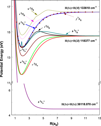
Figure 1. Potential energy curves of the H2  ,
,  ,
,  ,
,  ,
,  ,
, 
 ,
,  , and
, and  states. All are based on the BO potentials with adiabatic corrections calculated by Staszewska & Wolniewicz (1999, 2001) and Wolniewicz (1995b). All energy values are relative to the v = 0 and J = 0 levels of the
  state. Numerical values in cm−1 refer to the appropriate asymptotic limits. The asymptotic limits of the
  and
and  states are both H(1s)+H(2p), while that of the
  state is H(1s)+H(2s). For this reason, less precise values are given to the H(1s)+H(2
 ) as well as to the H(1s)+H(3
 ) dissociation limits. The peaks near 1.95a0 for the
  and
and  states arise from the large adiabatic corrections due to rapid changes in the electronic character in the avoided crossing region (Kolos & Rychlewski 1990a). Notice the vertical axis break between 6.5 and 11 eV.
Download figure:
Standard image High-resolution image3. Analysis and Results
3.1. Calculated Energy Levels
Table 1 compares the observed and current calculated energies of the  (
( ) levels of H2. The table lists the observed values and their differences with their theoretical counterparts. When the observed value is not available, the calculated energy, enclosed in parentheses, is listed.
Table 1.
Comparison of Calculated and Observed Energy Levels of the H2  (
( ) Statea
| N | v = 0 | O–C | v = 1 | O–C | v = 2 | O–C |
|---|---|---|---|---|---|---|
| 1 | 94941.58b | 0.19 | 97280.44 | 0.06 | 99497.17c | 0.09 |
| 2 | 95062.33b | 0.17 | 97395.47 | 0.04 | 99606.68c | 0.11 |
| 3 | 95242.37b | 0.19 | 97566.92 | 0.02 | 99769.87c | 0.11 |
| 4 | 95480.26b | 0.15 | 97793.46 | −0.05 | 99985.42c | 0.03 |
| 5 | 95774.38b | 0.16 | 98073.60 | 0.00 | 100251.85 | −0.01 |
| 6 | 96122.39 | −0.04 | 98405.06 | −0.10 | 100567.15 | −0.10 |
| 7 | 96522.52 | 0.18 | 98785.70 | −0.18 | 100929.11 | −0.23 |
| 8 | 96956.21d | −15.10 | (99213.24) | (101335.68) |
| N | v = 3 | O–C | v = 4 | O–C | v = 5 | O–C |
|---|---|---|---|---|---|---|
| 1 | 101595.19c | 0.01 | 103577.18e | −0.05 | 105445.40f | 0.27 |
| 2 | 101699.25c | −0.01 | 103677.11e | 1.11 | 105539.89f,g | 1.22 |
| 3 | 101854.37c | 0.02 | 103822.73f,g | −0.44 | 105677.77f,g | −0.25 |
| 4 | 102059.22 | −0.06 | (104017.58) | (105862.07) | ||
| 5 | 102312.45 | −0.02 | (104257.75) | (106089.37) | ||
| 6 | (102612.08) | (104541.87) | (106358.18) | |||
| 7 | (102955.97) | (104867.88) | (106666.52) | |||
| 8 | (103341.78) | (105233.51) | (107012.18) |
Notes.
aIn units of cm−1. Unless otherwise indicated, all observed values are from Dieke, as tabulated by Crosswhite (1972), after being lowered by 149.704 cm−1 as suggested by Lindsay & Pipkin (1997). O –C refers to the difference between the observed and current calculated energies. When the observed energies are not available, the current calculated values, enclosed in parentheses, are listed. bFrom Jungen et al. (1990). cEach of these levels is derived from one Q-branch line of the −
− transition obtained by Dabrowski & Herzberg (1984) and the adjusted
  energy of Dieke. The value agrees well with the adjusted
  value of Dieke.
dThis observed value is questionable. A value of 96585.3 cm−1 was obtained through the MQDT calculation of Ross et al. (2001).
eEach level is derived from just one Q-branch line frequency of the
value of Dieke.
dThis observed value is questionable. A value of 96585.3 cm−1 was obtained through the MQDT calculation of Ross et al. (2001).
eEach level is derived from just one Q-branch line frequency of the  −
− transition of Dabrowski & Herzberg (1984) and the lowered
  energy of Dieke. The derived value differs significantly from the corresponding adjusted
  energy of Dieke.
fDerived from just one Q-branch transition frequency of the
energy of Dieke.
fDerived from just one Q-branch transition frequency of the  −
− band observed by Dabrowski & Herzberg (1984) and the adjusted
  energy of Dieke. No corresponding
  value was given by Dieke.
gThe corresponding Q-branch line of the
value was given by Dieke.
gThe corresponding Q-branch line of the  −
− transition was found by Dabrowski & Herzberg (1984) to be blended.
Download table as: ASCIITypeset image
In comparison to their singlet-ungerade counterpart, the triplet-state energy levels are not as accurately and extensively determined. Most of the H2 energies of the low-lying triplet states were obtained from the extensive work of Dieke, as tabulated by Crosswhite (1972), and to a lesser extent, from Dabrowski & Herzberg (1984) and Jungen et al. (1990). The original energy values of Dieke, however, were found to be too high. Miller & Freund (1974) suggested that Dieke's values need to be reduced by 149.60 cm−1, while Lindsay & Pipkin (1997) suggested a reduction of 149.704 cm−1. Although the Lindsay & Pipkin (1997) reduction number may appear to be more accurate, the Miller & Freund (1974) number is more widely used (Ross et al. 2001). In any case, the difference of 0.10 cm−1 is less than the expected error in the measurement of Dieke. In Table 1, the number of Lindsay & Pipkin (1997) was applied to Dieke's listed values. Table 1 also lists a few indirectly observed  energy values, which are derived from the observed Q-branch frequency of the
  −
−  transition observed by Dabrowski & Herzberg (1984) and the corrected
  energy value of Dieke. Those indirect values are indicated by appropriate superscripts, c, d, and e. Superscript "c" indicates that the derived energy agrees with the corresponding
  value of Dieke, while "d" indicates a significant difference with Dieke's value. "e" indicates that the derived value was not observed in the measurements of Dieke. Although the corrected
  energies used to derive the
  energies are free from additional error beyond that of Dieke's measurement, the listed values with superscripts c, d, and e also include the experimental error of Dabrowski & Herzberg (1984). Moreover, the derived
  values are all made with just one Q-branch line, and some Q-branch lines, as indicated by the superscript f, were listed as blended by Dabrowski & Herzberg (1984). Although it is hard to assess the error of these indirectly determined energy levels, some of them can obviously have larger errors than the other listed
  values.
Except for N = 8 of the v = 0 level, the calculated energies of the first four vibrational levels agree with their experimental counterparts within ±0.25 cm−1. The differences between observation and calculation for the v = 4 and 5 levels are generally larger. For N = 2 of the v = 4 and 5 levels, the calculated energies are more than 1 cm−1 lower than the observation. Given the difficulty in the assessment of errors in the indirectly determined value, it is not clear that a large residual is primarily caused by the inaccuracy of the calculation. The  and other triplet-state energies were also calculated with MQDT by Ross et al. (2001). Their calculated values are generally 2 ∼ 4 cm−1 higher than the observation, primarily because they used less precise ab initio potentials and because the
  state has a significant valence character.
The calculated values in Table 1 are obtained with β = 0.055. A better agreement with the listed observations can be achieved with a smaller β value (such as 0.030). In a forthcoming paper, it will be shown that the β values of the  ,
,  ,
,  ,
,  , and
, and  states are between 0.08 and 0.11. A value of 0.03 would be too low when compared with these other states. Indeed, even β = 0.055 may turn out to be too low for higher (than observed) vibrational levels. The largest non-adiabatic shifts of the
  state are expected to occur in the v = 8−12 levels. The absence of the observed energies for these levels prevents β from being more accurately determined. To help future experimental measurements, Table 1 also lists the calculated energy levels of the v = 6−8 levels.
To further test the accuracy of the  potential energy curves, the
  energy levels of D2 and HD are also calculated. In going from H2 to the other isotopologues, the only change is the reduced mass (μ) of the nuclei and the introduction of mass asymmetry in the case of HD. The quantities in Equation (6) affected by the change of the mass are
  and
and  , both of which are inversely proportional to the nuclear reduced mass. Both the
  and
and  of D2 and HD can be obtained from their H2 counterparts with a simple reduced mass ratio.
  is obtained from Equation (8) with the appropriate
  . Other quantities are identical to their H2 counterparts. In the case of HD, there are two possible asymptotic limits: H(1s)+D(2p) and H(2p)+D(1s). Those two limits are separated by 3/(8
  ) au or 22.400 cm−1 after adjusting for the difference between the two non-adiabatic offsets mentioned earlier. Because the effect of the g–u symmetry-breaking Hamiltonian is neglected, the HD
  potential has the middle point of the H(1s)+D(2p) and the H(2p)+D(1s) energies as its asymptotic limit. When the g–u symmetry-breaking term is taken into account, the asymptotic limit of the
  state will likely turn out to be the H(2p)+D(1s) limit, while that of its interacting partner,
  , is likely to be the H(1s) + D(2p) limit. In the large R region, the potential used in the present work for the HD
  state is about 11.200 cm−1 higher than the exact value. The eigenvalue and eigenfunction are mostly determined by the magnitude and shape of the potential within ∼10 Å. Unless the level is really close to the asymptotic limit, the effect of the g–u symmetry-breaking Hamiltonian on the calculated energies is negligible.
Table 2 compares the observed and calculated D2 energy levels. As in Table 1, the values enclosed in parentheses are the calculated energies. Like H2, most of the measured values were made by Dieke (as tabulated by Freund et al. 1985) and by Jungen et al. (1992; see also Lavrov & Umrikhin 2008). The entries with a superscript c were derived by Ross et al. (2001) from the  −
− Q-branch frequencies observed by Dabrowski & Herzberg (1984) and the
  energies tabulated by Freund et al. (1985). Similar to H2, the expected experimental error is presumably a few tenths of 1 cm−1. Except for the apparent misassignment at N = 11 of the v = 2 levels, all differences between the observed and calculated numbers are significantly less than 1 cm−1. Once again, the residuals are nearly all positive, which suggests that the non-adiabatic correction in the low v levels are probably overestimated.
Table 2.
Comparison of Calculated and Observed Energy Levels of the D2  (
( ) Statea
| N | v = 0 | O–C | v = 1 | O–C | v = 2 | O–C | v = 3 | O–C |
|---|---|---|---|---|---|---|---|---|
| 1 | 95215.52b | 0.17 | 96897.10c | 0.34 | 98516.54c | 0.32 | 100075.35c | 0.30 |
| 2 | 95276.54b | 0.17 | 96956.09c | 0.36 | 98573.50c | 0.32 | 100130.25c | 0.20 |
| 3 | 95367.79b | 0.19 | 97044.15c | 0.25 | 98658.68c | 0.33 | 100212.48c | 0.20 |
| 4 | 95488.88b | 0.16 | 97161.28c | 0.34 | 98771.64c | 0.24 | 100321.62c | 0.20 |
| 5 | 95639.45b | 0.20 | 97306.30c | −0.10 | 98912.23 | 0.33 | 100457.41 | 0.34 |
| 6 | 95818.85b | 0.19 | 97480.05 | 0.30 | 99079.72 | 0.38 | 100618.98 | 0.28 |
| 7 | 96026.49b | 0.20 | 97680.61 | 0.25 | 99273.43 | 0.35 | 100806.05 | 0.33 |
| 8 | 96261.54b | 0.13 | 97907.77 | 0.26 | 99492.69 | 0.24 | 101017.71 | 0.26 |
| 9 | 96523.43 | 0.23 | 98160.72 | 0.30 | 99737.00 | 0.34 | 101253.55 | 0.41 |
| 10 | 96810.90 | 0.14 | 98438.51 | 0.31 | 100004.94 | 0.07 | 101512.82 | 0.85 |
| 11 | 97123.47 | 0.30 | 98740.21d | 0.26 | 100257.58e | −38.62 | (101793.06) | |
| 12 | 97459.43 | 0.03 | (99064.69) | (100609.68) | (102095.51) | |||
| 13 | 97818.66 | 0.23 | (99411.41) | (100944.35) | (102418.34) | |||
| 14 | 98199.37 | 0.20 | (99779.05) | (101299.16) | (102760.56) | |||
| 15 | 98600.75 | 0.24 | (100166.55) | (101673.10) | (103121.16) |
| N | v = 4 | O–C | v = 5 | O–C | v = 6 | O–C |
|---|---|---|---|---|---|---|
| 1 | 101574.69c | 0.27 | 103015.45c | 0.14 | 104398.65c | 0.12 |
| 2 | 101627.68c | 0.19 | 103066.63c | 0.15 | 104447.97c | 0.14 |
| 3 | 101707.15c | 0.32 | 103143.15c | 0.16 | 104521.64c | 0.11 |
| 4 | 101812.35c | 0.21 | 103244.67c | 0.15 | 104619.46c | 0.13 |
| 5 | 101943.26 | 0.25 | (103370.69) | (104740.85) | ||
| 6 | (102098.95) | (103521.01) | (104885.63) | |||
| 7 | (102279.36) | (103694.91) | (105053.09) | |||
| 8 | (102483.58) | (103891.74) | (105242.61) | |||
| 9 | (102710.90) | (104110.79) | (105453.50) | |||
| 10 | (102960.50) | (104351.29) | (105684.99) | |||
| 11 | (103231.53) | (104612.40) | (105936.29) | |||
| 12 | (103523.11) | (104893.26) | (106206.52) | |||
| 13 | (103834.29) | (105192.94) | (106494.81) | |||
| 14 | (104164.11) | (105510.51) | (106800.23) | |||
| 15 | (104511.58) | (105844.99) | (107121.84) |
Notes.
aIn units of cm−1. Unless otherwise specified, all observed values are from Freund et al. (1985). O–C refers to the difference between the observed and current calculated energies. When the observed energies are not available, the current calculated values, enclosed in parentheses, are listed. bFrom Jungen et al. (1992). cDerived by Ross et al. (2001) from the Q-branch frequencies of the −
− transitions obtained by Dabrowski & Herzberg (1984) and the
  energies given by Freund et al. (1985).
dFrom Lavrov and Umrikhin (2008)
eThis observed value is questionable. A value of 100257.58 cm−1 was obtained for this level using the MQDT calculation of Ross et al. (2001).
energies given by Freund et al. (1985).
dFrom Lavrov and Umrikhin (2008)
eThis observed value is questionable. A value of 100257.58 cm−1 was obtained for this level using the MQDT calculation of Ross et al. (2001).
Download table as: ASCIITypeset image
Table 3 compares the observed and calculated HD energy levels. Unlike the H2 and D2 cases, only about 30 levels of the HD  state have been measured. The observed data in the table are derived from Table 2 of Keiding & Bjerre (1987) and the absolute energy 97107.50 ± 0.30 cm−1 of the v = 1 and N = 1 level measured by Kim & Mazur (1995). Note that the value 97107.50 cm−1was listed in both Tables VI and VII of Kim & Mazur (1995) with a partial uncertainty of ± 0.10 cm−1. It was, however, incorrectly printed as 97105.50 ± 0.30 cm−1 in both the abstract and conclusion sections. The Keiding & Bjerre (1987) numbers were reported as the value relative to that of the v = 0 and N = 1 level. The fine and hyperfine interactions split each N level of the HD molecule into a number of closely spaced lines and could not be fully resolved by Keiding & Bjerre (1987). A primary error of 0.02 cm−1 was introduced when they took the peak frequency of the strongest component as the rotational transition frequencies. The overall error of the observed HD energy listed in the table is probably ±0.35 cm−1. All but two residuals listed in Table 3 are within the expected error limits. Like D2, all residuals are positive. Since H2, D2, and HD use an identical β value, the previous discussion on β for H2 also applies to the D2 and HD
  state. In both D2 and HD, the difference between observation and calculation generally becomes smaller as v increases. When the experimental values of the
  = 8 and 9 levels and the HD v > 4 levels become available, it is possible that the residuals will become negative. If the prediction turns out correct, it would justify the use of β = 0.055 or the use of even slightly higher values.
Table 3.
Comparison of Calculated and Observed Energy Levels of the HD  (
( ) Statea
| N | v = 0 | O–C | v = 1 | O–C | v = 2 | O–C | v = 3 | O–C |
|---|---|---|---|---|---|---|---|---|
| 1 | 95066.63 | 0.27 | 97107.50 | 0.23 | 99056.17 | 0.15 | 100914.99 | 0.09 |
| 2 | 95157.65 | 0.27 | 97194.78 | 0.23 | 99139.80 | 0.15 | 100995.07 | 0.09 |
| 3 | 95293.52 | 0.26 | 97325.07 | 0.23 | 99264.64 | 0.14 | 101114.60 | 0.09 |
| 4 | 95473.48 | 0.24 | 97497.62 | 0.21 | 99429.96 | 0.11 | 101272.87 | 0.06 |
| 5 | 95696.55 | 0.22 | 97711.48 | 0.19 | 99634.84 | 0.08 | 101469.00 | 0.04 |
| 6 | 95961.53 | 0.22 | 97965.49 | 0.18 | 99878.16 | 0.05 | 101701.89 | 0.01 |
| 7 | 96267.06 | 0.26 | 98258.35 | 0.22 | 100158.64 | 0.05 | 101970.32 | 0.03 |
| 8 | 96611.65 | 0.44 | 98588.58 | 0.36 | (100474.74) | (102272.79) |
Note.
aIn units of cm−1. All observed values are obtained from Table 2 of Keiding & Bjerre (1987) and E(v = 1,N = 1) = 97107.50(30) cm−1 from Tables VI and VII of Kim & Mazur (1995). Note that the E(v = 1,N = 1) value was incorrectly printed as 97105.50(30) cm−1 in both their abstract and conclusion (see also Ross et al. 2001). O–C refers to the difference between the observed and current calculated energies. When the observed energies are not available, the current calculated values that are enclosed by parentheses are listed.Download table as: ASCIITypeset image
The  energy levels of D2 and HD have also been calculated by Ross et al. (2001). The difference between the measured and their MQDT values for D2 are generally between −1.5 and −3.5 cm−1 and for HD between −2.6 and −2.9 cm−1.
The very good agreement between the current calculation and observation for H2, D2, and HD demonstrates the accuracy of the  potential energy curve and correct isotopic dependence of the empirical non-adiabatic correction in Equation (8). The calculated energies for the v = 0−10 and N = 1−15 levels of the H2, HD, and D2
  state are given in Table 9.
The  (
( ) energy levels have been accurately computed by Wolniewicz (2007), who used the
  of the
 state as the radiative correction of the
  state and
  +Erel(2s) (but with Erel(2s) = −0.42 cm−1, instead of −0.457 cm−1) as the relativistic correction. More importantly, Wolniewicz (2007) accurately computed the non-adiabatic correction of the
  state and demonstrated that nearly all non-adiabatic shifts of the low N levels arise from the coupling with the
  states. Except for the large-N levels, coupling with the
  states is negligible. A number of vibrational levels of the
  and
and  states lie between the vj = 8 level and dissociation limit of the
  state. The interaction among the three states leads to large non-adiabatic shifts for the
  state, especially for the vj > 8 levels. Consequently, the value of β for the
  state is unusually large. Moreover, because of the importance of localized coupling by the
  and
and  states, the non-adiabatic correction of the
  (
( ) levels cannot be accurately represented by a single β value. Although the v
  levels can be represented by β = 0.18−0.19, the non-adiabatic shifts of the v = 10−14 levels require β = 0.2−0.3.
Since the low v levels of the  state and their transitions to the low v levels of the
  state are the primary focus of the present investigation, the β parameter is set to 0.19. The measured
  energies are available only for the v = 0−7 levels (Crosswhite 1972; Jungen et al. 1990). The agreement between the current calculation and the previous measurement is similar to that between Wolniewicz's (2007) calculation and experimental measurement. For the v = 0−8 levels of the
  state, the differences between the present and Wolniewicz's (2007) calculations range from −0.19 to 0.31 cm−1. If β = 0.19 is used for all
  levels, the difference reaches as large as 1.68 cm−1 at the v = 12 and N = 9 level. Even though the present work may have used more accurate
  and
and  , the non-adiabatic energy obtained by Wolniewicz (2007) is generally more accurate than the present value.
3.2. FCFs, Transition Probabilities, Predissociation Rates, and Lifetimes
The refinement of the potential energy curves of the  ,
,  , and, to a lesser extent,
  states over those of Liu et al. (2016, 2017) increases the accuracy of the calculated transition probabilities in two respects. The first is that it obtained more accurate energies, which result in more accurate transition frequencies. Even though the error due to the neglect of non-adiabatic coupling in the previous calculation partially cancels when the difference is taken, a small error remains because of the difference in the magnitude of non-adiabatic coupling of the
  and
and  states. The error in the previous
  −
− transition frequency in some high v levels of the
  state can be as large as 4 cm−1. However, it is always less than 1.7 cm−1 in the present calculation. The frequency errors in the transition of low v levels are nearly always less than 1 cm−1. The improvement, however, does not necessarily apply to the
  −
− transition because the empirical non-adiabatic correction is inapplicable to the
  state. The second refinement is the more accurate vibrational wave functions from the solution of the Schrödinger equation, which results in more accurate matrix elements involving vibrational wave functions. The improvements are expected in FCFs, transition probabilities, and some matrix elements used to calculate the predissociation rate of the
  levels. The difference between the present and previous total
  −
− transition probabilities of Liu et al. (2017) ranges from 0.1% to 1%. The difference between the FCFs of the
  −
− and
and  −
− transitions is slightly smaller, in the range of 0.1% to ∼0.8%. Overall, while the present results are marginally more accurate, nearly identical results would have been obtained by using the potential energy curves of Liu et al. (2017).
The  −
− ab initio transition moment calculated by Staszewska & Wolniewicz (1999) is utilized for the calculation of the
  −
− transition probabilities. The transition moment is available for R up to 20a0. The value of the transition moment at 20a0 is already very small. It is further extrapolated to the asymptotic value of 0 by
  . As discussed in Liu et al. (2017), the M1 and E2
  −
− transition probabilities have fairly large uncertainties, due to the limited accuracy and R range of the transition moments of Chiu & Lafleur (1988). Both M1 and E2 transition moments are expected to vanish at large R. However, the Chiu & Lafleur (1988) transition moments failed to show any asymptotic behavior at the largest available R (10.021a0). Instead, both of their values peak at 10.021a0. To avoid a large uncertainty in the extrapolation, Liu et al. (2017) restricted the calculation of the M1 and E2 transitions to the
  and
and  levels of the
  state. To match the measured lifetimes of the metastable H2, HD, and D2 species measured by Johnson (1972), Liu et al. (2017) had to add a constant of 370 s−1 to the sum of the calculated total M1 and E2 transition probabilities of the vj = 0 level (and every other (vj, Nj) level). This added value is about 64% of the calculated total transition probability of the vj = 0 level. For the computation of emission spectra and kinetic energy distributions, the use of the constant offset is very inconvenient. In the present work, all of the calculated M1 and E2 transition probabilities are uniformly scaled up by a factor of 1.64. For the vj = 0 level, both methods give nearly identical results. For the other levels, the scaling will obviously produce higher emission yields and emission cross-sections than Liu et al. (2017). However, since the M1 and E2 transition probabilities are much smaller than the E1 transition probabilities and predissociation rates, the effect of the scaling is very small for the
  levels.
Because of the limited R range of the M1 and E2 transition moments of Chiu & Lafleur (1988), the emission spectra and kinetic energy distributions of the M1 and E2 transitions in the present investigation are restricted to the  and
and  levels only. The FCFs from the
  (vi = 0) level are significant only for the first several vj levels of the
  state. The sum of FCFs for the first 6, 9, and 12 vj levels are ∼0.84, ∼0.95, and ∼0.98, respectively. The restriction only has a small effect on the results reported in the present investigation.
The  −
− vibrational overlap integrals,
  , for the O-, P-, Q-, R- and S-branches of the vi = 0 and Ni = 0−15 levels (Table 4) and the Q-branch transition probabilities of the
  −
− band system for N up to 15 (Table 5) are given as supplementary material (see the Appendix). Only the Q-branch transition probabilities are given because the predissociation rates of the
  levels are more than four orders of magnitude greater than the total spontaneous emission rates.
Table 4.
Non-adiabatic Transition Energies and Vibrational Overlap Integrals of the  (
( )−
)− (
( ) Transitiona
| vj | Nj | vi | Ni | Eijb |
 c
c
|
|---|---|---|---|---|---|
| 0 | 1 | 0 | 0 | 94941.39 | 3.37399E–01 |
| 0 | 2 | 0 | 0 | 95062.16 | 3.31470E–01 |
| 1 | 1 | 0 | 0 | 97280.27 | −4.31154E–01 |
Notes.
aAn expanded list of this table is provided in the machine-readable table. bIn units of cm−1. cNote that the square of the vibrational overlap integral, , is also the rotationally dependent FCF.
Only a portion of this table is shown here to demonstrate its form and content. A machine-readable version of the full table is available.
Download table as: DataTypeset image
Table 5.
Energies, Transition Frequencies, Transition Probabilities, and Franck–Condon Factors of the H2  −
− Band Systemsa
| N'b |
 b
b
|
 b
b
|
 b
b
|
 c
c
|
Ea–Ecc | Ad | FCFe |
|---|---|---|---|---|---|---|---|
| 1 | 1 | 21 | 0 | 95143.03 | −23233.45 | 7.5535E–05 | 5.0951E–13 |
| 1 | 1 | 20 | 0 | 95143.03 | −23229.58 | 3.2277E–04 | 2.1784E–12 |
| 1 | 1 | 19 | 0 | 95143.03 | −23216.03 | 1.0323E–03 | 6.9803E–12 |
Notes.
aAn expanded list of this table is provided as a machine-readable table. b( ) and (
 ) always refer to the vibrational and rotational quantum numbers of the upper and lower states, respectively.
cBoth the lower state energy, E(
) always refer to the vibrational and rotational quantum numbers of the upper and lower states, respectively.
cBoth the lower state energy, E( ), and transition frequency, Ea–Ec, are in units of cm−1. Note that the transition frequency is always defined as the energy difference between the
  and
and  states.
dThe transition probability, A, is positive even when the transition frequency is negative.
eThe FCF is N dependent, i.e., FCF =
states.
dThe transition probability, A, is positive even when the transition frequency is negative.
eThe FCF is N dependent, i.e., FCF =  .
.
Only a portion of this table is shown here to demonstrate its form and content. A machine-readable version of the full table is available.
Download table as: DataTypeset image
3.3.
Excitation Function and Cross-sections

H2 excited to a  level completely predissociates. H2 excited to a
  level produces only a weak continuum emission. The long lifetime of the
  level further complicates the detection efficiency of the
  emission in any lab measurements. For this reason, all measured
  absolute excitation cross-sections are from the EEL investigations of Khakoo & Trajmar (1986), Wrkich et al. (2002), and Hargreaves et al. (2017), which give values of 14, 15, 16, 17.5, 20, 30, 40, and 60 eV. By using laser excitation of the electron-excited
  (
( ) levels of H2 to the
  state, and by detecting the enhancement of the continuum emission arising from the LIF of the
  −
− transition, Ottinger & Rox (1991) were able to measure ro-vibrationally resolved relative excitation functions of the
  (0)−
(0)− (vj = 0−3, N = 2) excitation from threshold energy to ∼22 eV. Ottinger & Rox (1991) also measured the relative population of the
  state as a function of electron energy using a TOF technique with a flight time of 60−70 μs. Mason & Newell (1986) also made a similar measurement earlier. The Mason & Newell (1986) data, however, have an incorrect asymptotic shape, which was likely caused by the presence of significant secondary electrons. Lee et al. (1993, 1996) calculated the excitation cross-sections for Nj = 2 of the
  (vj = 0−3) state and obtained reasonably good agreement with the LIF shapes of Ottinger & Rox (1991). More recently, Zammit et al. (2017) performed CCC calculations and achieved very good agreement with the EEL measurement of Khakoo & Trajmar (1986) at 30, 40, and 60 eV.
The LIF measurement of Ottinger & Rox (1991) suffered from a strong background that arises from complicated cascade dissociative emission processes due to the excitation of H2 by electrons to triplet levels higher than  . Possibly because of this interference and possibly because of the significant difference in the cascade excitation of the vj = 0, 1, 2, and 3 levels, the relative shape of the excitation function for the four levels are significantly different. They are also significantly narrower than the shape implied by the TOF measurement. For this reason, a reliable shape could not be extracted from LIF or TOF, nor their combination.
The relative excitation function in the present work was extracted from the excitation cross-section from Ni = 0 and 2 of the  (vi = 0) state to Nj = 2 of the vj = 0, 1, 2, and 3 levels of the
  state calculated by Lee et al. (1996). The sum of the excitation cross-sections that originated from the Ni = 0 and 2 levels in the range from 13 to 40 eV are displayed in Figures 1(a)–(d) of Lee et al. (1996). The relative magnitude of the Ni = 0
  = 2 excitation to the Ni = 2
  = 2 excitation, however, can be obtained from the differential cross-sections given in Figures 3 and 4 of Lee et al. (1996). The ratio at both 20 and 25 eV is about 1.0:4.0. The present investigation assumed that this ratio is independent of excitation energy and limited the summation in Equation (3) to r = 1 and 2 with
  = 0.80 and
  = 0.20. Nonlinear least-squares fits of cross-sections to the vj = 0, 1, 2, and 3 levels show that all four sets of cross-sections have close, but not exactly identical, shapes. The vj = 3 shape is noticeably different from those of the other three levels by ∼15% between 30 and 40 eV. (The extracted shape, however, approximately goes through the middle so that the residual for each level is roughly either −8% or +8%.) It is estimated that the error in digitizing data from small figures can introduce an error of 2% to ∼5%. There is also a possibility that the FCFs used by Lee et al. (1996) are somewhat different from the present values. When those two factors are taken into account, the difference is probably reduced to 8% to ∼11%. Nevertheless, it is best to consider the derived excitation function as the average shape of the four sets of calculated cross-sections that are weighted by the present FCFs.
The ratios of the collisional strength parameters Cm/C6 (m = 0−4) and the absolute value of C5 listed in Table 6 are obtained directly from the calculated cross-section of Lee et al. (1996). The absolute value of C6 is determined by normalizing the 40 eV  state model cross-section to the corresponding EEL cross-section of Khakoo & Trajmar (1986). The applicable range of excitation functions is conservatively estimated to be from threshold energy to ∼70 eV. These parameters, along with the rotationally dependent FCFs listed in Table 4, allow one to calculate the model excitation cross-section from threshold energy to ∼70 eV. Any renormalization to a different cross-section value at a different energy can be achieved by a simple adjustment of the absolute value of C6.
The Lee et al. (1996) calculated shapes agree reasonably well with the LIF shapes of the vj = 0, 1, 2, and 3 levels measured by Ottinger & Rox (1991). The agreement between the extracted shape with its LIF counterpart is somewhat similar. For this reason, the only comparison between the TOF shape and the EEL shapes of Khakoo & Trajmar (1986), Wrkich et al. (2002), and Hargreaves et al. (2017) is presented here. It is important to note that the TOF measurement for the metastable H2 was obtained after a 60−70 μs flight time. If it is assumed that a steady-state population of H2 had been achieved in the electron collision chamber of Ottinger & Rox (1991), the population at t = 0, defined as the time when the excited H2 exits the interaction region, is

The excitation rate,  , can be obtained by first calculating the
  described in Section 2.1, using the extracted excitation function, and then partitioning the rate into the those of the fine-structure levels,
  , with normalized (2Jj + 1) degeneracy ratios.
  is the total decay rate of the fine-structure level obtained in the previous section. The number of particles at the level (
 ) that reached the detector after a flight time t = τ is simply

 is then summed over the (
 ) levels to obtain the population of the
  state of H2 at time τ. Due to the partition of
  , each F1, F2, and F3 fine-structure component is weighted with the normalized (2Jj+1) degeneracy in the summation. The calculation is repeated for a range of excitation energies. The relative value of the
  state population after a flight time τ is directly comparable to the TOF measurement of Ottinger & Rox (1991).
Figure 2 compares the TOF shape (blue circles) obtained by Ottinger & Rox (1991) with the model TOF shape (red line). Both traces have been normalized at their peak. The flight time in the Ottinger & Rox (1991) measurement is between 60 and 70 μs. The model assumes a flight time of 65 μs. There is very good agreement between the observation and model below 25 eV. Between 35 and 50 eV, the model is consistently lower than the observation. Part of the reason can be the presence of secondary electrons in the TOF measurement that lead to additional excitation of H2. In principle, secondary electrons become possible once the excitation energy reaches above 27.2 eV. However, if a large amount of metastable  H2 is present, the primary electrons with energy higher than ∼15.4 eV, in principle, can ionize the metastable species and produce secondary electrons that can excite H2 from the
  state to the
  state. As the lifetimes of the F1 and F3 fine-structure components of the H2
  (v = 0) metastable species are between 950 and 1040 μs (Liu et al. 2017), it is possible that a significant number of the
  (v = 0) species were generated in the collision chamber. The black trace of Figure 2 shows the normal
  excitation cross-section that would correspond to the TOF relative population at either τ = 0 or in the absence of the lifetime variation with (
 ). The green dot shows the TOF cross-section obtained by Mason & Newell (1986). As mentioned, their cross-section at a high energy, being nearly constant, was probably due to the presence of a significant number of secondary electrons.

Figure 2. Comparison of the relative excitation cross-sections of the  state. The blue dots are from the TOF measurement of Ottinger & Rox (1991), which was made after a 60 to ∼70 μs flight time. The green squares are the TOF measurements of Mason & Newell (1986) with a flight time of ∼20 μs. The black trace is the
  excitation cross-section calculated from the excitation function extracted from the theoretical cross-section of Lee et al. (1996). It assumes that all
  levels have identical lifetimes. The red trace assumes a steady-state
  population in the interaction region (t = 0) and a 65 μs flight time to reach the detector. The updated lifetimes obtained in the present investigation, which differ from those of Liu et al. (2017) by 0.5%–2%, have been used to model the population at the
  levels at t = 65 μs. All data sets have been normalized at their peak values.
Download figure:
Standard image High-resolution imageThe FCF of the  (0)−
(0)− (0) band is ∼0.116. Therefore, the excitation rate to the
  (0) level is fairly large. As Table 6 of Liu et al. (2017) shows, the lifetime of the
  (0) level is at least a factor of 5−7 longer than that of the higher vibrational levels. The TOF signal of Ottinger & Rox (1991) is thus entirely dominated by H2 at the
  (0) level through the smaller total decay rate in the denominator of Equation (9) and in the exponential decay factor of Equation (10). Moreover, since the lifetime of the F1 and F3 components far exceeds that of F2, the population in those two components of the H2
  (0) level far exceeds their F2 counterpart. The red trace of Figure 2, obtained with slightly refined total decay rates of the
  state, is in excellent agreement with the TOF measurement of Ottinger & Rox (1991) from threshold energy to ∼25 eV. As mentioned earlier, the difference between experimental TOF data and the red model trace above 25 eV can be attributed to the presence of secondary electrons in the experiment, which appears to be supported by the excellent agreement with the (relative) EEL cross-section of Khakoo & Trajmar (1986) and the black trace in Figure 3, generated from an identical model excitation function. It is important to note that a model trace, based on the decay rates of Liu et al. (2017), after normalization to the peak cross-section, is indistinguishable from the red trace shown in Figure 2.

Figure 3. Excitation and emission cross-sections of the  state. The green diamonds, purple circles, and red squares denote the original EEL excitation cross-sections of Wrkich et al. (2002), Khakoo & Trajmar (1986), and Hargreaves et al. (2017), respectively. The brown trace with upper triangles is the CCC calculation of Zammit et al. (2017). The black line represents the present model excitation cross-section that is normalized to the 40 eV value of Khakoo & Trajmar (1986). The red and blue lines show the corresponding cross-sections of the
  and
and  components, respectively. The cyan trace refers to the emission cross-section of the
  state, which is a sum of the
  −
− emission by the magnetic dipole (M1) and electric quadrupole (E2) transitions and the
  −
− −
− emission by the electric dipole (E1) transitions (see the text). Note that only the bottom half of the error bar in the 20 eV cross-section of Wrkich et al. (2002) is shown and 1 MB = 1 × 10⁻¹⁸ cm−2.
Download figure:
Standard image High-resolution imageThe black trace of Figure 2 is obtained by assuming that the decay rate of every  level is independent of the vj and Nj quantum numbers. Because the normalization is at the peak value, the black trace is also equivalent to a 100% detection efficiency in the time domain for every H2 molecule excited to the
  state. The black trace clearly has very poor agreement with the TOF measurement of Ottinger & Rox (1991). The difference between the red and black traces essentially reflects the different weights on the excitation rate to each
  levels. Although not as sensitive as the direct measurement of Johnson (1972) and Berg & Ottinger (1994), the excellent agreement between the red trace and the TOF measurement of Ottinger & Rox (1991), from threshold energy to ∼25 eV, also shows that the calculated predissociation rates and spontaneous transition probabilities appropriately account for the difference in various decay rates in the TOF measurement.
3.4. Kinetic Energy Distributions
The predissociation of the  state takes place by strong electronic Coriolis interaction with the
  state. Consequently, its rate (see Table 7) is at least four orders of magnitude faster than the spontaneous decay rate. Any H2 molecule excited to the
  levels can be considered to predissociate completely. The H(1s) production rate by
  (
( ) excitation simply equals twice that of its excitation rate,
  ), in Equation (2).
The predissociation of the  state occurs through a much weaker electron spin interaction with the
  state. Its predissociation rate (see Table 8) is several orders of magnitude smaller than the rate of the
  state and is comparable to the spontaneous decay by E1, M1, and E2 transitions. The production rate of H(1s) atoms by the
  (
( ) levels equals the product of twice that of its excitation rate and its predissociation yield. The predissociation yield can be obtained from the calculated predissociation rate and lifetime given in Section 3.2. Figure 4 compares the production rates of H(1s) atoms by the predissociation of the
  and
and  states at 18 eV and 300 K.

Figure 4. Comparison of the relative predissociation rates and their distributions from the  and
and  excitations at room temperature (300 K) and 18 eV excitation energy. Note that the H(1s) production rate is twice that of the predissociation rate of H2. The red trace, with an offset of 0.07, refers to the predissociation via the
  state while the black trace denotes that through the
  state. The H atom production rate via the
  predissociation is ∼68% greater than that via the
  state at 18 eV. The average Ek of the H(1s) atoms produced by the
  and
and  predissociation channels are both ∼4.1 eV/atom. Note that the kinetic energy distribution of the predissociation of the
  (
( ) levels is intrinsically sharp. The FWHM for the fast predissociating
  state ranges from ∼10−3 to ∼4 cm−1, depending on the v and N quantum numbers. Because of much longer lifetimes, the widths for the
  levels are much narrower than those of the
  levels. The discrete Ek production rates shown in the figure have been convolved with a Gaussian profile with a uniform FWHM of 2 meV (∼16 cm−1). The vibrational quantum numbers of the predissociating levels are labeled with magenta lines on top.
Download figure:
Standard image High-resolution imageThe equations for calculating the Ek distributions of the  −
− M1 and E2 spontaneous emission channels are identical to those given in Liu et al. (2010a), while the equation for the Ek distribution of the
  −
− −
− cascade channel has been presented in Liu et al. (2016). The Ek distribution of the
  and
and  predissociation channels can be obtained by simply normalizing their total H(1s) production rates to unity. Like the previous work (Liu et al. 2016), the Ek of each decay channel given in the present work is individually normalized. Figure 5 shows the Ek distributions from the predissociation of the
  state at 13, 15, and 20 eV excitation energies.
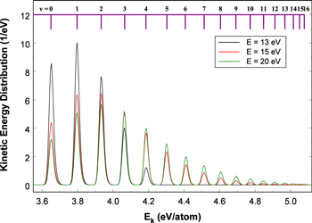
Figure 5. Comparison of the kinetic energy distribution of H(1s) atoms produced from the predissociation of the electron-excited  state of H2 at 13, 15, and 20 eV excitation energies. The predissociation includes those of both the
  and
and  channels, and the sum of the distribution is normalized to unity at each energy. The black, red, and green traces refer to the Ek distributions from excitation at 13, 15, and 20 eV, respectively. The H2 temperature is assumed to be 300 K. All traces have been convolved with a Gaussian profile with an FWHM of 25 meV (∼200 cm−1) in order to help the visualization.
Download figure:
Standard image High-resolution image4. Discussion
The theoretical energies of the  state of H2, D2, and HD, obtained from the potential energy curves discussed in Section 2.2, agree very well with the experimentally derived energies listed in Tables 1–3. Except for N = 2 of the v = 4 and 5 levels (and misassigned levels), all other differences between the observed and calculated energies are substantially smaller than 1.0 cm−1. Because the experimental values were derived from multiple sets of measurements, it is difficult to assess the uncertainties of the various measured values. Given the good agreement in the other observed levels, it is possible that the 1.11 and 1.22 cm−1 residuals at the two N = 2 levels are mostly due to experimental uncertainties.
If the experimental energies are accurately measured, any properly calculated energies will be no lower than their measured counterparts. All (O – C) entries in Tables 1–3 would have been either negative or zero. However, most of the residuals in the tables are positive. There are several reasons for the positive residuals. The first and probably the least important reason is the experimental uncertainty. The second is the inaccuracy of  and
and  , which are extrapolated from the corresponding quantities of either the H2
  or
or 
 states. Even though they are accurate at large R, the actual
  and
and  may be different from the extrapolated values in the region of a few angstroms around Re, which has a much greater impact on the calculated energy. The most important reason for the positive residual is the approximate nature of
  in Equations (7)–(8) and the adopted value of β. As mentioned, a value of β = 0.055 was used to obtain the calculated energies in Tables 1–3. If β = 0.030 had been used, the overall absolute value of the residuals would have been generally smaller, and most of the residuals would have been negative. An implicit assumption of
  in Equations (7)–(8) is that the state considered is sufficiently separated from other electronic states so that any localized couplings are negligibly weak. This assumption, however, is less likely true for the levels close to the dissociation limit.
Regardless of the many investigations of the  state, the measured
  energy values of only a few low v levels are available (see Tables 1–3). This is likely caused by the difficulty in populating the high v levels of the
  state and the small spontaneous transition probabilities of the
  levels. In general, only a few of the lowest v levels of the triplet states have significant Franck–Condon overlap with the
  (v = 0) level. Moreover, transitions between triplet states are strongly dominated by diagonal (Δv = 0) bands. The restriction of the Franck–Condon overlap applies to both schemes, i.e., by electron impact excitation and by
  and alkaline metal vapor reaction. It can be noted that the low pressure discharge with a large spectrometer, equipped with classical photographic plates, utilized by Roncin & Launay (1994) and Abgrall et al. (1993a, 1993b, 1993c, 1994) was able to detect emission from the v = 33 and 34 levels of
  , which have FCFs of 1.1 × 10⁻³ and 8 × 10⁻⁴ from the
  (0) level. The v = 6–8 levels of the
  state, with corresponding FCFs of (5–∼2) × 10−2, have either not been detected or assigned, presumably because the
  −
− transition probabilities are smaller than their
  counterparts. In this regard, it is interesting to note that many lines in Dieke's hydrogen wavelength tables (Crosswhite 1972) were not assigned. It is hoped that the values in parentheses, calculated with β = 0.055, listed in Tables 1–3 and in Table 9, will be useful for future investigations of higher v levels. It is anticipated that the error of the calculated value is less than 1 cm−1 for levels sufficiently below the 1s+2p dissociation limit.
The potentials described in Section 2.2 make it possible to calculate the great majority of the discrete ro-vibrational levels of the  ,
,  ,
,  ,
, 
 ,
,  , and
, and  states of H2 and its isotopologues and the
  state of
  and its isotopologues with an accuracy of better than 1 cm−1 by solving the one-dimensional Schrödinger equation. The derived (empirical) non-adiabatic nuclear wave function can be used to evaluate the appropriate matrix elements required by physical parameters such as FCFs, predissociation rates, and transition probabilities. When computed on the same basis, the non-adiabatic FCFs and total transition probabilities of the E1
  −
− and the M1 and E2
  −
− transitions in the present work agree with their adiabatic counterparts in Liu et al. (2017) within 0.06% to ∼1.3%. The two sets of lifetimes for the
  and
and  levels differ by no more than 2% (when the M1 and E2
  −
− transition probabilities are scaled in the same way).
There are small differences (<3%) between the total decay rates obtained in the present work and those of Liu et al. (2017). The differences are primarily caused by the adjustment of the M1 and E2  −
− transition probabilities. In Liu et al. (2017), a constant offset of 370 s−1 is added to the total M1 and E2 transition probability of each ro-vibrational level whereas a multiplication factor of 1.64 is applied in the present investigation. Although both approaches produce nearly identical lifetimes for the vj = 0 levels, the present lifetimes for the vj > 0 levels are generally shorter. A small difference in the two sets of lifetimes is also caused by a somewhat more accurate non-adiabatic nuclear wave function in the present work. The different approaches will obviously lead to a small difference in the emission branching ratio and emission yield; however, it has a negligible effect on the kinetic energy distribution because the distributions for various decay channels are individually normalized.
There are also small (0.1% to ∼1%) differences between the total dipole transition probabilities of the  −
− band given in Table 1 of Liu et al. (2017) and those obtained in the present calculation. The difference is entirely caused by the use of slightly more accurate potentials in the present study, which produce slightly more accurate vibrational wave functions and transition frequencies.
Three sets of EEL cross-sections of the  state are available. Khakoo & Trajmar (1986) measured the cross-section at 20, 30, 40, and 60 eV with reported relative errors of 19%–21%. Wrkich et al. (2002) reported this same cross-section at 17.5, 20, and 30 eV with estimated errors of 22%–24%. The difference between the two sets of cross-sections, however, is significantly larger than the joint error margins (see Figure 3). The more recent cross-section of Hargreaves et al. (2017) is primarily for the threshold energy region and is available only at 14, 15, 16, and 17.5 eV. The original Wrkich et al. (2002), Khakoo & Trajmar (1986), and Hargreaves et al. (2017) cross-sections, along with their error bars, are shown in solid green diamonds, purple circles, and red squares, respectively, in Figure 3. The Wrkich et al. (2002) cross-section at 20 and 30 eV is significantly greater than the corresponding Khakoo & Trajmar (1986) cross-section. If the Wrkich et al. (2002) cross-section is reduced by 42%, its 20 and 30 eV values would agree well with that of Khakoo & Trajmar (1986). However, its 17.5 eV cross-section would fall from 10.9 MB to 6.4 MB.
The black trace of Figure 3 shows the room temperature (300 K) model excitation cross-section of the  state after normalizing to the 40 eV EEL cross-section of Khakoo & Trajmar (1986). The fact that the extrapolated 60 eV model cross-section agrees well with the EEL cross-section of Khakoo & Trajmar (1986) suggests the correctness of the asymptotic form of the excitation function in Table 6. The
  model cross-section can be separated into the
  and
and  components, which are shown by the red and blue lines, respectively. As noted by Jonin et al. (2000), the larger cross-section of
  than
than  is primarily due to the presence of the R-branch excitation from the J = 0 level of the
  (0) state in the former and the absence of the Q-branch excitation from the same level in the latter. Although H2 excited to the
  state fully predissociates, a portion of H2 excited to the
  state spontaneously decays by E1
  −
− −
− radiative cascade, and by M1 and E2
  −
− emission. The cross-section of those three emission channels is represented by the cyan line.
The ratio of the value of the cyan line to that of the black line in Figure 3 is the band emission yield of the  −
− excitation. The M1 and E2
  −
− transitions that had been scaled up by a factor of 1.64 contribute ∼30% to the total
  emission. The uncertainties of the M1 and E2 transition moments noted earlier as well as the different scaling clearly have some impact on the accuracy of the band emission yield. As most of the emission arises from the low v levels of the
  state, the band emission yield tends to decrease with the excitation energy. Between 11.8 and 15 eV, the yield ranges from 20% to 17%. As the excitation energy moves above 18 eV, the yield approaches a value of (15.9 ± 0.2)%.
The EEL cross-section of Wrkich et al. (2002) drops by a factor of ∼2.3 in going from 20 eV to 17.5 eV. The model cross-section, in contrast, increases by ∼22%. As a result, the model cross-section is about a factor of 2.7 larger if both the model and Wrkich et al. (2002) cross-sections are normalized at 30 eV. It is not clear what causes the sharp drop in the EEL cross-section of Wrkich et al. (2002) in going from 30 eV and 20 eV to 17.5 eV. A possible explanation will be given below. It can be noted that the corresponding 17.5 eV cross-section of Hargreaves et al. (2017), 12.8 MB, obtained with much more accurate FCFs, is about 17% greater than the corresponding Wrkich et al. (2002) value. Furthermore, the Wrkich et al. (2002) data appear to suggest that the  cross-section peaks around 20 eV. However, all LIF and TOF shapes measured by Ottinger & Rox (1991) suggested that the peak cross-section is around 16−17 eV. Finally, as indicated by Figure 2, the present model excitation function agrees very well with the TOF measurement from threshold energy to 22 eV. A sharp reduction of the
  cross-section around 17.5 eV, as suggested by Wrkich et al. (2002), would invalidate all measurements of Ottinger & Rox (1991).
In addition to the model and EEL cross-sections, Figure 3 also shows the CCC cross-sections of Zammit et al. (2017). The shape of the present model's cross-section also agrees well with that of the CCC cross-section when the excitation energy is above 23 eV. The agreement in the two shapes below 23 eV, however, is not very good. In general, the model cross-sections below 20 eV are higher than both the measured EEL and calculated CCC cross-sections. The 20 and 30 eV Wrkich et al. (2002) cross-sections are ∼29% larger than the corresponding implied cross-sections of Lee et al. (1996), which themselves are about 29% higher than the black trace in Figure 3.
Even though the  state cross-sections of Wrkich et al. (2002) are currently recommended values (Yoon et al. 2008), there are some indications that the EEL cross-section, at least at 20 eV, is too high. The sum of the total triplet excitation cross-section and singlet-gerade breakup cross-section can be obtained from the difference between the total dissociation cross-section of Corrigan (1965) and the sum of the breakup cross-sections by ionization and singlet-ungerade excitation. The ionization breakup cross-section includes both dissociative and nondissociative channels and has been accurately measured by Straub et al. (1996), which has subsequently been updated by Lindsay & Mangan (2003). The singlet-ungerade breakup cross-section includes dissociation, predissociation, and dissociative emission channels. The total dissociation cross-section and a partial predissociation cross-section have been reported by Liu et al. (2012, 2009). If the dissociation and predissociation of the singlet-gerade states such as
  are completely neglected, the difference gives an upper limit of the total triplet cross-section. At 20 eV, the sum of the Khakoo & Segura (1994)
  cross-section and the Wrkich et al. (2002)
  cross-section already slightly exceeds the upper limit. When the
  EEL cross-section is added, the sum of the first three triplet states exceeds the 20 eV upper limit by ∼17%.
It should noted that the calculated  cross-sections obtained by Lima et al. (1988) at 20 and 30 eV are about 100% and 40% higher than the Wrkich et al. (2002) EEL measurements. The fact that the EEL cross-sections at these energies need to be further decreased probably suggests that several factors in the experimental normalization of the differential cross-section (DCS) data need to be re-examined. First, the DCSs at larger scattering angles can be lowered by about 10%–20% using the elastic scattering DCSs of Muse et al. (2008), instead of those of Khakoo & Trajmar (1986). In addition, it is possible that the determination of the transmission of the spectrometer to the helium ionization continuum was overestimated in Wrkich et al. (2002). Finally, the FCFs used by Wrkich et al. (2002) are not as accurate as those of Hargreaves et al. (2017) or those listed in Table 4. The less accurate FCFs used in the overall unfolding of the EEL spectra could have overestimated the DCSs, which, however, has yet to be ascertained, as the most recent work of Hargreaves et al. (2017) covered only 14−17.5 eV in energy. In any case, the large change in the
  EEL cross-section from 17.5 eV to 20 eV remains an open question.
Since the model excitation function agrees well with the TOF measurement of Ottinger & Rox (1991) from threshold energy to ∼22 eV, and since the model cross-section is greater than the EEL measurement between 14 and 17.5 eV, the cascade excitation of the  state in the TOF measurement can be significant. The
  ,
,  ,
,  , and
, and  states, being the next few higher gerade states, are expected to be the most likely cascading states. The low v levels of these triplet-gerade states have a large Franck–Condon overlap with the
  (0) level. Within the
  ,
,  ,
,  , and
, and  −
− band transitions, these low v levels also primarily decay to the low vj levels of the
  state, which, in turn, were preferentially detected in the TOF measurement. However, since H2 excited to the
  ,
,  , and
, and  states can also decay to the
  state, and, especially, to the much lower
  state, the emission branching ratio from these three states to the
  state is actually small. A preliminary calculation by one of the authors shows that less than one-sixth of the H2 excited to the N = 1 level of the
  (0) state decays to the
  state. The
  state is different because, in the absence the
  −
− and
and  −
− ,
,  , and
, and  non-adiabatic couplings, the spontaneous
  −
− and
and  transitions would be impossible. As a result, the
  −
− transition often has a much larger branching ratio. The same preliminary calculation also shows that more than 61% of H2 excited to the N = 2 level of the
  (0) state decays to the N = 1 and 3 levels of the
  (0) state. Thus, the
  −
− transition should be the most important contributor to the cascade excitation of the
  state.
The threshold energy of the  (0) state is ∼13.95 eV (and 13.85−13.9 eV for
  (0),
(0),  (0), and
  (0)). If the shape of the excitation functions of these triplet-gerade states are similar to that of the
  state, their excitation cross-sections and the cascade components to the
  state are expected to peak around 19.5 eV. The fact that the 20 eV model cross-section is ∼18% lower than the Khakoo & Trajmar (1986) cross-section suggests that cascade excitation of the
  state is unlikely an important factor for the difference between the model and EEL cross-sections below 20 eV. The uncertainties in the EEL measurements and model shape function are likely the primary cause of the difference.
Figure 4 shows the relative atomic hydrogen production rate by predissociation (which is twice that of the predissociation rate) for each ( ) level of the
  state at room temperature at 18 eV excitation energy. Even though the lifetimes of the low N levels of the
  state range from 3.1 ns to a few hundredths of a nanosecond (Martín & Borondo 1988; Liu et al. 2017), the intrinsic width of the kinetic energy peak is much narrower than what can be shown in a figure. Consequently, the rate of all
  levels have been convoluted by a Gaussian profile with a uniform FWHM of 2 meV. The black line in the lower panel of the figure shows the H production rate of the
  level while the red line in the upper panel, after being shifted up by 0.07, represents the rate of the
  state. The vibrational quantum number of each peak is shown by the magenta labels on the top. Although most of the H atoms are produced with Ek below 4.5 eV, atomic fragments with energy as high as 5.1 eV can also be produced by the predissociation of the
  state. The average Ek of the
  and
and  channels are both ∼4.1 eV/atom. Since the
  state has a larger excitation cross-section than that of the
  state (see the red and blue lines of Figure 3) and is 100% predissociated, the Ek production rate by the excitation to the
  state is about 68% higher than that to the
  state.
H atoms with  are produced from the predissociation of the
  levels near the H(1s)+H(2p) dissociation limit. Any population distribution of the H2
  state that favors excitation into these high-lying levels will also increase the production of fast-moving H atoms. Since the high-lying levels also include the low vj but high Nj levels of the
  state, it is thus possible to produce a significant number of fast H atoms by excitations from the high Ni levels of the
  (0) state. This requirement is somewhat different from the dissociation by the
  state, where the production of a significant number of H atoms with Ek ≥ 5 eV requires a significant population of H2 at vibrationally excited (vi ≥ 2) levels of the
  state (Shemansky et al. 2009).
The kinetic distribution of the predissociation of the  state can be obtained by summing the production rate of atomic hydrogen over the v and N quantum numbers and normalizing the sum to 2 (as two H atoms are formed for each H2 predissociated). The black, red, and green traces in Figure 5 show the Ek distribution at excitation energies of 13, 15, and 20 eV, respectively. As discussed, the Ek distribution of the predissociation is very sharp. The distributions shown in the figure have been convoluted by a Gaussian profile with an FWHM of 25 meV. In the threshold region, a low-energy excitation preferentially excites the low v levels, which produces relatively slow H atoms. The low Ek peaks dominate the distribution. As excitation energy increases, the fraction of H2 excited to high v levels increases while that to the low v levels decreases. The high Ek peaks in the distribution become more important. In general, a higher excitation energy produces a greater fraction of fast H atoms. However, above ∼25 eV, the variation of the cross-section due to the difference in the threshold energy becomes very small and the appearance of the Ek distribution is insensitive to further increase of the excitation energy.
The black, red, and green lines in Figure 6 show the Ek distribution of H atoms produced by the spontaneous emissions of H2 from the  state by E1, M1, and E2 transitions, respectively. The
  state in the figure is assumed to be populated by 17 eV electron excitation at room temperature and each distribution is individually normalized. In the case of the E1 cascade dissociative transition, excitation to all (vj, Nj) levels were considered. However, for both M1 and E2 transitions, only excitation to the vj = 0−11 and Nj = 1−8 levels are considered. As can be seen, the E1 transition generates the fastest moving H atoms, with an average Ek of ∼1.3 eV. The M1 transition produces atoms with an average Ek of ∼1.0 eV. The E2 transition gives rise to the slowest H atoms with an average Ek of only ∼0.8 eV. Apart from being proportional to the square of the appropriate matrix element of the transition moment, the E1 and M1 continuum transition probabilities are proportional to the cubic power of the emission frequency while the E2 transition probability is proportional to the penta power of the frequency. If the dependence of the E1, M1, and E2 transition moments on the internuclear distance is similar, the E2 transition will be much more likely to occur in the high frequency and low Ek region than its E1 and M1 counterparts, which is the reason why the E2 transition (green trace) gives rise to the slowest H atoms. The E1
  −
− −
− channel involves two sets of electric dipole transitions. Its comparison with the M1
  −
− transition is not as straightforward and will not be discussed here.
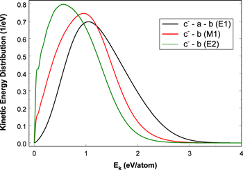
Figure 6. Comparison of kinetic energy distributions of H(1s) atoms produced from dissociative emission from the  state to the
  state at 17 eV excitation energy and 300 K. The black line shows the result of the
  −
− −
− radiative cascade by electric dipole (E1) transitions. The red line shows the distribution from the direct
  −
− spontaneous dissociation by magnetic dipole (M1) transition. The green line shows the distribution from the same spontaneous transition by electric quadrupole (E2). Note that all distributions have been normalized to unity even though the magnitudes of the three dissociative emission mechanisms are very different. The Ek distributions of the M1 and E2 transitions are calculated based on excitation to the vj = 0−11 and Nj = 1−8 levels of the
  state only, while the distribution of the E1 transition is based on excitation to all (vj, Nj) levels. The average Ek for the black, red, and green distributions at 17 eV excitation energy are 1.28, 1.00, and 0.80 eV/atom, respectively.
Download figure:
Standard image High-resolution imageSince the relative population of H2 at various ( ) levels of the
  state depends on the excitation energy, the Ek distributions of the E1, M1, and E2 transitions also have some dependences on the excitation energy. Figure 7 shows the Ek distributions of the
  −
− −
− E1 cascade and the dissociative emission induced by excitation of the
  state of H2 at various excitation energies. As the excitation energy increases, the probability density,
  , becomes broader and, correspondingly, has lower peak heights. Furthermore, the location of its maximum density value and average Ek both shift to lower value. The trend can be explained by the similarity of the potential energy curves and the dependence of the transition probability on the transition frequency. Because of the close resemblance of the
  and
and  potential energy curves, the FCF of the
  (vj)−
(vj)− (vk) transition is nearly a
  function (see the last column of Table 5). This means that, in the absence of other decay channels, the cascade excitation rate of the
  (
( ) level is almost equal to the sum of the direct excitation rate to the
  (
( ) level from the
  state. From an
  (
( ) level, the sum of the photon energy and the kinetic energy of two outgoing hydrogen atoms is equal to the energy difference between the
  (
( ) levels and the H(1s)+H(1s) limit in Figure 1. However, since the transition probabilities are proportional to the cubic power of the transition frequencies, the dissociative emission preferentially yields a higher-energy photon and a lower Ek of the H(1s) atoms. Moreover, the higher the
  (
( ) energy, the stronger the preference. When the excitation energy is very low, only the low vj levels of the
  state, and thus the low v levels of the
  state, can be populated. Those low v levels tend to give lower transition frequencies and, thus, higher Ek. Furthermore, since fewer (
 ) levels are populated with low excitation energy, the distributions of the photon energy and Ek are narrower, which, upon normalization, gives a greater peak height. In contrast, as the excitation energy increases, more (
 ) levels can be populated, which gives a broader peak but a lower peak height. The increased significance of the excitation to high (
 ) levels also produces a lower Ek value of hydrogen atoms.
Table 6.
Collision Strength Parameters of the  State Excitation Functiona
| Parameter | Value |
|---|---|
| C0/C6 | −6.0777629 |
| C1/C6 | 2.8731985 |
| C2/C6 | 6.6750929 |
| C3/C6 | 85.579083 |
| C4/C6 | 22.865149 |
| C5 | 1.0546218 |
| C6b | 0.82659174 |
Notes.
aSee Equation (5) for the definition of the collision strength parameters and the state excitation function. The applicable range of the excitation function is from threshold energy to ∼70 eV.
bThe absolute value of C6 is obtained by normalizing the 40 eV
state excitation function. The applicable range of the excitation function is from threshold energy to ∼70 eV.
bThe absolute value of C6 is obtained by normalizing the 40 eV  state model excitation cross-section to the corresponding EEL cross-section measured by Khakoo & Trajmar (1986).
Download table as: ASCIITypeset image

Figure 7. Excitation energy dependence of the Ek distribution of H(1s) atoms produced from the  −
− excitation, followed by the
  −
− −
− cascade dissociative emission. The initial
  H2 population distribution is assumed to be thermal with a temperature of 300 K. When the excitation energy is very low, the cascade dissociative emission from the low vj levels dominates, which produces a larger fraction of fast H atoms. As the excitation energy increases, the importance of the low vj levels decreases, a smaller fraction of fast H atoms is produced, and the peak of the Ek distribution gradually shifts to the low-energy region. As the excitation energy moves above 20 eV, the Ek distribution becomes insensitive to any increase of energy. See the text for an explanation of the excitation of low vj levels that produce a greater fraction of faster H(1s) atoms.
Download figure:
Standard image High-resolution imageFigures 8 and 9 also present the three-dimensional plots of the Ek distributions of the M1 and E2 transitions at various excitation energies. They both show an excitation energy dependence of the Ek distribution similar to that of the E1 transition in Figure 7. As noted earlier, the penta power dependence of the E2 transition probabilities on the frequency gives rise to a narrower peak width and greater peak height, and a lower averaged Ek.
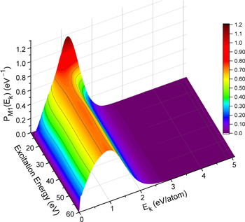
Figure 8. Kinetic energy distribution of H(1s) atoms produced from the  −
− excitation, followed by the
  −
− magnetic dipole (M1) dissociative emission. The initial H2 population distribution is assumed to be thermal with a temperature of 300 K. Only the excitations to the vj = 0−11 and Nj = 1−8 levels of the
  state are used to calculate the M1 kinetic energy distribution. Note that nearly all H(1s) atoms are produced with Ek less than 3 eV, and the average Ek of the distribution decreases slightly with the excitation energy.
Download figure:
Standard image High-resolution image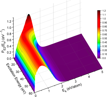
Figure 9. Kinetic energy distribution of H(1s) atoms produced from the  −
− excitation, followed by the
  −
− electric quadrupole (E2) dissociative emission. The initial H2 population distribution is assumed to be thermal with a temperature of 300 K. Only the excitations to the vj = 0−11 and Nj = 1−8 levels of the
  state are used to calculate the E2 kinetic energy distribution. Note that nearly all H(1s) atoms are produced with Ek less than 3 eV, and the average Ek of the distribution decreases moderately with the excitation energy.
Download figure:
Standard image High-resolution imageFor all three Ek distributions, the most significant excitation energy dependence is in the threshold region. Once the excitation energy moves above 19 to ∼20 eV, the Ek distributions are insensitive to additional increases in the excitation energy (see Figure 7).
The average energy deposited into an H2-dominated atmosphere for each H2 molecule excited to an excited state can be roughly estimated from the average Ek of the H atoms of each dissociation channel and the branching ratios. Since each Ek distribution depends on the excitation energy of electrons and the H2 population distribution of the  state, the average Ek values given below assume an excitation of room temperature (300 K) H2 by mono-energetic electrons with energy above 19 eV. The predissociation of the
  state produces hydrogen atoms with kinetic energy between 3.6 and 5.1 eV per atom, with an average Ek of ∼4.1 eV. The
  −
− cascade, followed by the
  −
− dissociative emission, both by E1, produces H(1s) atoms with an average Ek of ∼1.3 eV. The
  −
− dissociative emission by M1 and E2 generate H(1s) atoms with average Ek of ∼1.0 and ∼0.8 eV, respectively. On the whole, slightly less than 75% of the excessive energy of the
  state is released in the form of photon energy. When all dissociative channels are combined, the excitation of the
  state produces H(1s) atoms with an average Ek of ∼3.6 eV per atom. This number may change somewhat when more accurate M1 and E2 transition moments of the
  −
− band become available. If the H2 population distribution in the upper atmosphere of Saturn, for instance, is thermal (i.e., Boltzmann) and the temperature is not much higher than 300 K (<1500 ∼ 2000 K), each H2 molecule excited to the
  state deposits ∼7.1 eV of energy into the atmosphere. It is important to note that this 7.1 eV number is not applicable if the H2 population deviates significantly from a thermal distribution.
Even though the calculations of the present investigation are carried out at the ( ) state-specific level, the large number of ro-vibrational levels makes it impractical to show the results on an individual basis. A Boltzmann distribution at 300 K is conveniently chosen to present the results. A deviation from the distribution introduces a different set of weights to the calculated quantities of the (
 ) levels. For the low-energy electron excitation, the impact of the higher (vi,Ni) levels, which have smaller threshold energies, is enhanced via the excitation function (Equation (5)). The cross-section also changes with the (
 ) dependence of the FCF,
  . In general, the variations of FCFs, transition probabilities, lifetimes, and
  predissociation rates with N is much smaller than those with v.7
Moreover, the N dependence, when averaged over many rotational levels, tends to cancel out. Approximately 98% and 95% of H2 is in the vi = 0 level in a thermal distribution at 1500 and 2000 K, respectively. As long as the temperature is lower than 2000 K, the Ek distribution probably does not deviate significantly from that of 300 K. High-temperature thermal distribution or non-thermal distribution introduces a large population at the vibrationally excited state. The Ek distribution is expected to be significantly different from that of 300 K. A large difference is also expected at the top of planetary thermospheres and in the interstellar medium where the collisional deactivation rate is slow, and a significant H2 population is in the high vi levels. In any case, if the electron flux and energy distribution, and the H2
predissociation rates with N is much smaller than those with v.7
Moreover, the N dependence, when averaged over many rotational levels, tends to cancel out. Approximately 98% and 95% of H2 is in the vi = 0 level in a thermal distribution at 1500 and 2000 K, respectively. As long as the temperature is lower than 2000 K, the Ek distribution probably does not deviate significantly from that of 300 K. High-temperature thermal distribution or non-thermal distribution introduces a large population at the vibrationally excited state. The Ek distribution is expected to be significantly different from that of 300 K. A large difference is also expected at the top of planetary thermospheres and in the interstellar medium where the collisional deactivation rate is slow, and a significant H2 population is in the high vi levels. In any case, if the electron flux and energy distribution, and the H2  (
( ) population distribution are known, the physical parameters obtained in the present investigation enables one to obtain the H atom Ek release rate by electron impact
  −
− excitation.
On average, the excitation to the  state gives out more kinetic energy than any other triplet state on the basis of each H2 excitation. As mentioned, ∼7.1 eV excitation energy is converted into kinetic energy for each H2 excited to the
  state. The
  −
− excitation, on average, converts only about 2.3−2.4 eV into kinetic energy (Liu et al. 2010a). The
  −
− excitation gives rise to only about 3.3 eV kinetic energy (Liu et al. 2016). Even though 100% of the excessive electronic energy in the direct
  state excitation is converted into kinetic energy, the
  (0)−
(0)− excitation releases, on average, only ∼5.7 eV of energy. The ultimate energy release rate, of course, also depends on the excitation rate to each (
 ) level of an electronic state, which, in turn, is a convolution of the electron energy distribution and the excitation function. The
  state, with the largest low-energy cross-section and the lowest threshold, clearly dominates in the energy deposition rate. The
  state, with the second largest triplet cross-section and second lowest threshold, is the second most important state.
The triplet emission in the vacuum UV region nearly always arises from dissociative emission to the  state. H2 excited to a triplet-gerade state primarily decays to the
  state by the E1 process and gives out continuum emission. H2 excited to a triplet-ungerade state dissociates by either directly decaying into the
  state via weak M1 and E2 processes or, more likely, to the
  state, followed by the
  transition. Because the triplet continuum emission is spread over a very wide wavelength range, its intensity is weak and is often masked by the much stronger discrete and continuous Lyman (
 ) band emission. The emission spectrum observed by Cassini UVIS in Saturn's primary atomic H source region shows significant continuum intensity in the 1650−1900 Å region. Since the Lyman continuum on the red side of 1670 Å is very weak (Abgrall et al. 1997), the continuum emission from triplet excitation of H2 by electrons is thus responsible for the observed intensities. The investigation of the contribution of various triplet excitations to the continuum emission between 1670 and 1900 Å is thus very critical for inferring the total emission and excitation rates from the UVIS observations. Figure 10 compares the relative spectral intensities of the E1, M1, and E2 emission channels of the
  state with those from the direct excitation of the
  state at 20 eV excitation energy. The E2 emission, shown by the blue line, is the weakest and peaks at around 1650 Å. The M1 emission, shown by the red line, is the second weakest and has a broad peak that reaches maximum around 2300 Å. The E1 cascade emission, shown by the magenta line, is the strongest of the three and peaks near 2100 Å. The emission from the direct
  excitation, shown by the black line and calculated from the Ajello & Shemansky (1993) excitation function, far dominates over those from the
  state excitation. The continuum emission from the
  −
− excitation, whose magnitude is somewhat uncertain in the threshold region, has been presented elsewhere (Liu et al. 2016). It should be noted that the relative emission intensities from the different electronic states are all somewhat uncertain because of the errors in the excitation cross-sections of triplet states. It is clear that the shape, peak location, and magnitude of each emission channel are different and proper consideration of each emission channel is very important to obtain accurate emission and excitation rates from the observed continuum emission.
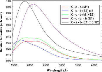
Figure 10. Comparison of continuum emission spectra of H2 from various channels at 300 K and 20 eV excitation energy. The red line denotes the  −
− (also
(also  −
− ) emission via magnetic dipole (M1), while the blue line refers to the same transition via electric quadrupole (E2). The green line is the sum of the two components. The purple line represents the
  −
− −
− (also
(also  −
− −
− ) emission via electric dipole (E1). The black line is the emission due to the direct excitation of the
  state obtained by Liu et al. (2010a) at the same energy. Note that the intensity of the E2 emission has been increased by a factor of 5, while that of the direct
  emission has been reduced by a factor of 8. Because of the limitation of the M1 and E2 transition moments discussed in the text, both M1 and E2 emission spectra are only from the v = 0−11 and N = 1−8 levels of the
  state. Also note that the intensities of the continuum transitions by electric quadrupole, magnetic dipole, electric dipole, and the direct excitation peak at ∼1650, ∼2300, ∼2100, and ∼1850 Å, respectively.
Download figure:
Standard image High-resolution imageThe analysis described in this paper was carried out at Space Environment Technologies. A portion of the work was carried out at the Jet Propulsion Laboratory, California Institute of Technology, under a contract with the National Aeronautics and Space Administration (NASA). We gratefully acknowledge financial support through NASA's Planetary Atmospheres (PATM) and Astrophysics Research and Analysis (APRA) programs, through the National Science Foundation's AST program (#1518304), and through a Cassini UVIS contract with the University of Colorado.
Appendix:
Table 4 provides a partial list of the calculated excitation energies (in cm−1) and the vibrational overlap integrals  of the
  −
− transition, which are useful for the calculation of excitation cross-sections and rates from an excitation function. An expanded table that lists the excitation energies and vibrational overlap integrals from the vi = 0 and Ni = 0−15 levels of the
  state to the (
 ) levels of the
  state with ΔN = 0, ±1, and ±2 is given in machine-readable format. Note that a simple squaring of the vibrational overlap integral produces the so-called rotationally dependent FCFs. Because of the approximate nature of the empirical non-adiabatic correction, the calculated energy of the vi = 0 and Ni = 0 level of the
  state with β = 0.1199 is −0.055 cm−1, instead of the expected 0 cm−1. The tabulated excitation energies are all shifted upwards by 0.055 cm−1 (which is equivalent to upwardly shifting all calculated
  energies so that the energy of the vi = 0 and Ni = 0 level is 0 cm−1). In this way, the excitation energy is consistent with the values listed in Table 1. Table 4 also neglects any coupling of the
  state with the
  states (Λ doubling), so that the
  and
and  levels are always degenerate.
Table 7.
Predissociation Rates, Kinetic Energy Release, and FCFs of the  (
( ) Levelsa
| v | N | Pred. Width | Pred. Rate | Ek | FCFb |
|---|---|---|---|---|---|
| 0 | 1 | 1.678E–03 | 3.160E+08 | 7.29315 | 1.360E–06 |
| 0 | 2 | 4.745E–03 | 8.938E+08 | 7.30813 | 1.354E–06 |
| 0 | 3 | 8.687E–03 | 1.636E+09 | 7.33045 | 1.346E–06 |
Notes.
aThe units of the predissociation width, predissociation rate, kinetic energy, and FCF are cm−1, s−1, eV, and 1/hartree, respectively. bFCF = .
.
Only a portion of this table is shown here to demonstrate its form and content. A machine-readable version of the full table is available.
Download table as: DataTypeset image
Table 8.
Predissociation Rates of the  (
( ) Levelsa
| v | N | F1 | F2 | F3 | Averageb |
|---|---|---|---|---|---|
| 0 | 1 | 62.3 | 4610.9 | 1768.0 | |
| 0 | 2 | 60.5 | 4284.8 | 22.9 | 1461.1 |
| 0 | 3 | 55.0 | 3979.4 | 32.6 | 1357.8 |
Notes.
aThe unit of the predissociation rate is s−1. bAverage predissociation rate of the F1, F2, and F3 fine-structure components based on (2J+1) degeneracy.Only a portion of this table is shown here to demonstrate its form and content. A machine-readable version of the full table is available.
Download table as: DataTypeset image
Table 5 provides a partial list of the calculated non-adiabatic energies, transition frequencies, transition probabilities, and FCFs of the  −
− band system. An expanded, machine-readable table that lists these quantities for N up to 15 is also given. Note that (
 ) and (
 ) always refer to the vibration and rotation quantum numbers of the upper and lower states, respectively, while the transition frequency is always defined as
  . Thus, if the frequency is negative, the transition refers to an emission from
  to
to  , and
, and  =
=  . In contrast, if the frequency is positive, the transition is an emission from
  to
to  , and
, and  =
=  . The spontaneous transition probabilities, A (in units of 1/s), always take positive values. The FCF is given as
  . Note that the FCFs for the
  =
=  transitions are near unity and the diagonal bands are the strongest transitions of the
  −
− band system. The total transition probability of a (
 ) level can be obtained by summing the Q-branch transition probabilities over appropriate lower (
 ) levels. Although the present total transition probability is marginally more accurate than that given in Liu et al. (2017), the expected error in the total transition probability is similar. For the v = 1−9 levels, it is expected to be less than 5%. For the
  levels, the error is expected to be less than 10%. See Liu et al. (2017) for a discussion on the accuracy of the
  −
− dipole transition moment.
Table 7 shows a partial list of the calculated predissociation widths, predissociation rates, kinetic energy release, and FCFs of the  state. The (predissociation) lifetimes of the
  (
( ) levels are simply inverses of the rates. Since the
  (
( ) and
) and  (
( ) states are considered to be degenerate, both of them have the same Ek and
  . The calculated results for vj = 0−21 and N up to 15 levels are available in machine-readable format.
Table 8 shows a partial list of the calculated predissociation rates of the F1, F2, and F3 fine-structure components of the  state. The average predissociation rate of the components, based on 2J+1 degeneracy, is also listed. Because of the limitation of some fine-structure interaction parameters used for the calculation, predissociation rates are given only for the vj = 0−6 and N = 0−15 levels.
Finally, as a supplement to Tables 1–3, Table 9 presents a partial list of the calculated  (
( ) energies for H2, HD, and D2 molecules. An expanded table on the calculated energies of the v = 0−10 and N = 1−15 levels for all three molecules is available in machine-readable format.
Table 9.
Calculated  (
( ) Energies of the H2, HD, and D2 Moleculesa
| Molecule | v | N = 1 | N = 2 | N = 3 | N = 4 | N = 5 |
|---|---|---|---|---|---|---|
| H2 | 0 | 94941.39 | 95062.16 | 95242.18 | 95480.11 | 95774.22 |
| H2 | 1 | 97280.27 | 97395.32 | 97566.79 | 97793.40 | 98073.49 |
| H2 | 2 | 99497.08 | 99606.57 | 99769.75 | 99985.38 | 100251.86 |
| H2 | 3 | 101595.18 | 101699.26 | 101854.35 | 102059.27 | 102312.47 |
| H2 | 4 | 103577.22 | 103675.99 | 103823.17 | 104017.58 | 104257.75 |
Note.
aIn units of cm−1. (This table for the v = 0–10 and N = 1–15 levels of the H2, HD, and D2 molecules is available in machine-readable form.)Only a portion of this table is shown here to demonstrate its form and content. A machine-readable version of the full table is available.
Download table as: DataTypeset image
Footnotes
- 4
The two-electron Darwin term of
vanishes for the state. The one-electron term was accurately computed by Jamieson et al. (2000). Its mass–velocity term for R > 5a0 was also calculated by Piszczatowski et al. (2008). An attempt to use the combination of the state terms and some terms for the of the state was not successful. - 5
The method described here is an obvious approximation as it violates the indistinguishability of two 1s electrons of the
state. - 6
Since it is assumed that the
state had a asymptotic limit, the comparison is made on the long-range potential with the R = potential value of the H(1s) + H() limit. If the , and at R = for were used, the difference would be 8.8 × 10⁻² cm−1. - 7
The predissociation of the
state is an exception because the rate is formally proportional to . Such a strong rotational dependence, however, does not lead to any difference because even the lowest Nj levels of the state completely predissociates.


