Rotational Spectra in 29 Vibrationally Excited States of Interstellar Aminoacetonitrile

The number of unidentified lines in the millimeter and submillimeter wave surveys of the interstellar medium has grown rapidly. The major contributions are due to rotational transitions in excited vibrational states of a relatively few molecules that are called the astrophysical weeds (Goldsmith et al. 2006; Fortman et al. 2010). To address this problem, assignments and analyses of rotational spectra in the low-lying vibrational states of not yet identified astrophysical species are needed. The necessary data to deal with spectral lines from astrophysical weeds species can be obtained from detailed laboratory rotational measurements in the microwave and millimeter wave region.

One of the interstellar molecules to be considered is aminoacetonitrile, which has received a particular amount attention due to its implication in chemical synthesis of the smallest amino acid, glycine (Rimola et al. 2010; Ugliengo et al. 2011). First detection of aminoacetonitrile was based on more than 80 ground vibrational state transitions in the line survey of the hot core of massive star-forming region Sgr B2(N) (Belloche et al. 2008), where molecules with –NH₂ and/or –CN groups are abundant. This region is well known for the elevated temperature of the gas, which suggests that a considerable part of the observed lines belong to rotational transitions in excited vibrational states. Indeed, a large amount of emission lines coming from the excited vibrational states were detected in Sgr B2 (Belloche et al. 2013). While the ground-state rotational spectra of aminoacetonitrile and its amino deuterated isotopologues are well characterized from the microwave up to the THz frequency region (MacDonald & Tyler 1972; Pickett 1973; Brown et al. 1977; Bogey et al. 1990; Motoki et al. 2013), the spectroscopic data in excited vibrational states are missing. Neither rotational spectra of ¹³C isotopic species have been reported to date. Therefore, the key to success in future astrophysical identification of more lines of aminoacetonitrile lies in new laboratory assignments and measurements for direct comparison of laboratory frequencies with those from astrophysical weeds.

In the present work, new spectroscopic measurements and analysis of aminoacetonitrile have been performed in frequency ranges 26–40 GHz, 75–115 GHz, and 170–240 GHz. Stark-modulation microwave and frequency-modulation millimeter wave spectroscopies made it possible to identify the pure rotational transitions of 29 different excited vibrational states belonging to fundamentals, overtones, and combination states of the low-frequency torsional and bending modes. Such a large number of excited vibrational states has never been analyzed in any other observed interstellar molecule. In addition, ground-state rotational transitions of two ¹³C isotopic species were measured in their natural abundances. More than 2000 new lines are reported, which should facilitate astronomers' further observations of aminoacetonitrile in the interstellar medium.

Stark-modulation microwave and millimeter wave spectroscopies results were fundamental in the analysis of the rotational spectra of aminoacetonitrile in excited vibrational states. A scheme of our upgraded Stark-modulation spectrometer used in the present investigation is shown in Figure 1. The spectrometer covers the frequency range from 12 to 110 GHz using either backward wave oscillators (BWOs) or an Agilent synthesizer as microwave sources. In the first case, three BWOs are available, providing the following frequency outputs: 12.5–18 GHz, 18–26.5 GHz, and 26.5–40 GHz (see Figure 1). The frequency stabilization of the BWOs is achieved by means of a phase-lock loop using an external frequency synthesizer, harmonic mixer, and signal synchronizer with a constant IF of 20 MHz. The signal from stabilized BWOs enters directly the 1.95 m long X-band waveguide or an additional passive multiplier V-2X (Spacek Labs) can be implemented to double the output of the highest-frequency BWO (see Figure 1). In the second case, an Agilent synthesizer (250 kHz–20 GHz) is used to drive the amplifier-multiplier chains WR15 and WR10 (VDI, Inc.) with multiplication factors of four and six to reach the frequency ranges of 50–75 GHz and 75–110 GHz, respectively. Another option is to connect passive multipliers Ka-2X, Q-3X, and V-4X (Spacek Labs) that allow us to record the spectra in the 26–40 GHz, 33–50 GHz, and 50–75 GHz regions, respectively. Modulation voltages up to 3000 V with a 33.3 kHz modulation frequency can be applied to the septum of the waveguide. A Stark-modulated signal is detected by solid-state zero-bias Schottky-diode detectors (50–110 GHz) or HP crystal detectors (12.5–50 GHz), pre-amplified and send to a lock-in amplifier where the phase-sensitive detection is applied.

Zoom In Zoom Out Reset image size

The frequency-modulation millimeter wave spectrometer was described elsewhere (Daly et al. 2014) and was used to record the spectra from 75 to 115 and from 170 to 240 GHz. The spectrometer is based on the cascaded multiplication of the synthesizer frequency by a set of active and passive multipliers (VDI, Inc.) and in this case the harmonic multiplication factors of 6 and $12=6\times 2$ were applied. In the lower-frequency region, detection was made with Schottky-diode detectors (VDI, Inc.) after two passes of radiation through the cell. The rotational spectra above 170 GHz were collected using a quasi-optical detector (VDI, Inc.) at a single pass configuration (see Daly et al. 2014 for details). The synthesizer output was frequency modulated at f = 10.2 kHz and the modulation depth  was between 20 and 40 kHz. A second derivative shape of the lines resulting from 2f detection was fitted to the Gaussian profile function and the uncertainty of the line center frequency was estimated to be better than 50 kHz.

The sample of liquid aminoacetonitrile was obtained commercially and was used without any further purification. Rotational spectra were recorded at room temperature and a pressure of approximately 15 μbar.

Aminoacetonitrile is a near prolate asymmetric top ($\kappa =-0.96$) with a C_s symmetry and two non-zero dipole moment components of $| {\mu }_{a}| =2.577$ (7) D and $| {\mu }_{b}| =0.5754$ (10) D (Pickett 1973). A large ${\mu }_{a}$ component is responsible for the intense a-type R-branch transitions that clearly dominate the room-temperature rotational spectrum. These transitions are interspersed by significantly weaker, but still observable, b-type R-branch and Q-branch transitions.

Around each ground-state line, many satellite lines attributable to pure rotational transitions in excited vibrational states were easily observed, as shown in Figure 2 for the ${4}_{13}\leftarrow {3}_{12}$ transition. Stark-modulation spectroscopy constitutes a definitive tool in the identification of rotational transitions in excited vibrational states (see, for example, Daly et al. 2013, 2015; López et al. 2014; Cernicharo et al. 2016; Kolesnikova et al. 2016). When a molecule is exposed to both microwave radiation and a square-wave modulation electric field, Stark negative lobes shifted with respect to the unperturbed line are observed in the spectrum. As shown in Figure 2(a), those satellite lines having the same pattern (circled in Figure 2(a)) as the ground-state line can be assigned to the same rotational transition in an excited vibrational state. For the vibrational assignment of these satellite lines, harmonic frequencies of the four lowest vibrational modes of aminoacetonitrile ${\nu }_{11}$ $(A^{\prime} )$, ${\nu }_{18}$ $(A^{\prime\prime} )$, ${\nu }_{17}$ $(A^{\prime\prime} )$, and ${\nu }_{10}$ $(A^{\prime} )$ associated with C–C$\equiv {\rm{N}}$ bending, NH₂–torsion, NH₂–CH₂–torsion, and N–C–C bending motions were calculated at the MP2/6-311++G(d, p) level of the theory (Gaussian09 package, Frisch et al. 2009). Harmonic frequencies together with normal coordinate displacement vectors are shown in Figure 3(a). The vibrational satellite pattern was modeled on the basis of the estimated changes of rotational constants relative to the ground-state values. This was done using the ab initio calculated first-order vibration-rotation constants ${\alpha }_{i}$ that define the well-known vibrational dependence of rotational constants ${B}_{v}={B}_{e}-{\sum }_{i}{\alpha }_{i}({v}_{i}+1/2)$, where B_v and B_e substitute all three rotational constants in a given excited state and in equilibrium, respectively. v_i is the vibrational quantum number of the ith vibrational mode. The modeled pattern is shown in Figure 2(b). The good matching in positions and intensities along with a similar Stark pattern constitute conclusive proof in the identification of rotational transitions in ${v}_{11}=1$, ${v}_{18}=1$, ${v}_{17}=1$, and ${v}_{10}=1$ excited states. Second excited states ${v}_{18}=2$ and ${v}_{17}=2$ were then readily found. Finally, combination states $({\nu }_{11}=1,{\nu }_{18}=1$) and $({\nu }_{11}=1,{\nu }_{17}=1$) were also identified by means of linear combinations of corresponding changes in their rotational constants. A total of eight excited vibrational states were characterized in Stark spectra. These constitute only a part of the plethora of vibrational states produced by the four low-lying modes, as shown in the manifold of levels in Figure 3(b).

Zoom In Zoom Out Reset image size

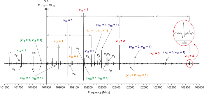
Zoom In Zoom Out Reset image size

On this basis, in a next step of the investigation, the millimeter wave spectrum between 75 and 240 GHz was recorded. As shown in Figure 4 for the ${11}_{110}\leftarrow {10}_{19}$ transition, a very rich satellite pattern was also observed. After a straightforward transfer of the line assignment from the Stark spectra to this higher frequency region, additional satellite lines v₁₁ = 2, 3, 4 belonging to successive excitations of the lowest frequency mode ${\nu }_{11}$ $(A^{\prime} )$ were easily assigned. In the absence of serious perturbations, such progressions are expected to show almost equidistant behavior of transition frequencies, which is shown in Figure 4 for the ${\nu }_{11}$ $(A^{\prime} )$, ${\nu }_{18}$ $(A^{\prime\prime} )$, and ${\nu }_{17}$ $(A^{\prime\prime} )$ low-frequency modes. Similar behavior allowed the identification of the combination states progressions (${v}_{11}=1,{v}_{18}=1$), (${v}_{11}=2,{v}_{18}=1$), (${v}_{11}=3,{v}_{18}=1$) and (${v}_{11}=1,{v}_{17}=1$), (${v}_{11}=2,{v}_{17}=1$). Additional (${v}_{18}=1,{v}_{17}=1$), (${v}_{18}=1,{v}_{10}=1$), and (${v}_{11}=1,{v}_{10}=1$) combination states could be also extracted from the records leading to 17 excited states found.

Zoom In Zoom Out Reset image size

Pursuing the detailed analysis, assignments of rotational transitions in another 12 excited states were achieved. These new excited states were labeled as v_a, v_b, ..., v_l. These states might be attributable to the remaining unassigned states depicted in Figure 3(b) or even to states above 1000 cm⁻¹. Based on the predicted changes in the values of rotational constants, v_c and v_i can be tentatively assigned to first quanta of ${\nu }_{16}$ $(A^{\prime\prime} )$ and ${\nu }_{9}$ $(A^{\prime} )$ calculated at 904 and 855 cm⁻¹, respectively. Other plausible assignments are collected in Table 3.

All of the measured rotational transitions for each of the 29 excited vibrational states were analyzed using the standard Watson's S-reduced Hamiltonian (Watson 1977) in I^r representation given by

$$\begin{eqnarray}{H}_{\mathrm{Rot}}^{(v)} & = & {{AJ}}_{a}^{2}+{{BJ}}_{b}^{2}+{{CJ}}_{c}^{2}-{D}_{J}{J}^{4}-{D}_{{JK}}{J}^{2}{J}_{a}^{2}-{D}_{K}{J}_{a}^{4}\\ & & +{d}_{1}{J}^{2}({J}_{+}^{2}+{J}_{-}^{2})+{d}_{2}({J}_{+}^{4}+{J}_{-}^{4})+{H}_{J}{J}^{6}+{H}_{{JK}}{J}^{4}{J}_{a}^{2}\\ & & +{H}_{{KJ}}{J}^{2}{J}_{a}^{4}+{H}_{K}{J}_{a}^{6}+{h}_{1}{J}^{4}({J}_{+}^{2}+{J}_{-}^{2})\\ & & +{h}_{2}{J}^{2}({J}_{+}^{4}+{J}_{-}^{4})+{h}_{3}({J}_{+}^{6}+{J}_{-}^{6}),\end{eqnarray} \tag{ 1 }$$

where A, B, C are the rotational constants, D_J,... d₂ are quartic, and H_J,... h₃ are sextic centrifugal distortion constants. The need for the sixth order terms depends on the excited states data sets. Resulting spectroscopic constants for the first and higher excited states of four lowest normal vibrational modes are given in Table 1, while those for combination states and v_a, v_b, ... v_l states are summarized in Tables 2 and 3, respectively. Experimentally measured frequencies are collected in Table 4. It must be noted that rotational transitions with higher J and K_a than those given in Tables 1–3 were also observed, however, they could not be treated within the semi-rigid rotor model applied in this work and were not included. Figure 3(b) shows that many states may be involved in mutual interactions as a result of proximity of their vibrational energy levels. Hence, multiple perturbations in their pure rotational spectra are expected and reflected in departures of the values of their centrifugal distortion constants with respect to those for the unperturbed ground state. Despite this, in the context of future astrophysical observations, the spectroscopic data provided for the most populated excited states are of enough precision to model spectra toward interstellar sources.

Table 1.  Spectroscopic Constants of Aminoacetonitrile in the First and Higher Successive Excitation States of Four Lowest Frequency Normal Vibrational Modes in Comparison with the Ground State (S-reduction, I^r-representation)

Constant	Unit	G.S.a	${v}_{11}=1$ b	${v}_{18}=1$ b	${v}_{17}=1$ b	${v}_{10}=1$
A	MHz	30246.4887 (10)c	30018.1544 (62)	30627.7386 (71)	30143.698 (10)	30630.93 (34)
B	MHz	4761.06254 (14)	4776.36759 (43)	4769.29434 (62)	4764.23280 (41)	4752.4590 (23)
C	MHz	4310.74857 (14)	4316.76886 (41)	4314.62273 (64)	4316.43101 (36)	4302.8937 (22)
DJ	kHz	3.06687 (11)	3.06106 (33)	3.03301 (35)	3.06103 (31)	3.04255 (76)
DJK	kHz	−55.2945 (14)	−50.298 (10)	−57.563 (14)	−55.0031 (56)	−55.430 (23)
DK	kHz	714.0755 (78)	558.80 (23)	862.77 (15)	694.86 (39)	714.0755d
d1	kHz	−0.673533 (41)	−0.67563 (27)	−0.67519 (50)	−0.67163 (14)	−0.6723 (16)
d2	kHz	−0.0299382 (96)	−0.019352 (27)	−0.039801 (99)	−0.026261 (49)	−0.0237 (10)
HJK	Hz	−0.12406 (51)	−0.2523 (82)	0.294 (13)	−0.1134 (33)	...
HKJ	Hz	−2.7126 (81)	...	...	−2.643 (12)	...
h1	Hz	0.003872 (15)	0.00434 (13)	0.00225 (27)	0.0038722d	...
${\sigma }_{\mathrm{fit}}$ e	kHz	41	48	46	40	61
${N}_{\mathrm{lines}}$ f	⋯	⋯	215	199	226	84
${J}_{\min }/{J}_{\max }$	⋯	1/74	6/40	8/39	8/37	8/26
${K}_{a,\min }/{K}_{a,\max }$	⋯	0/23	0/9	0/7	0/16	0/7
Constant	Unit	${v}_{11}=2$ b	${v}_{11}=3$	${v}_{11}=4$	${v}_{18}=2$	${v}_{17}=2$
A	MHz	29785.189 (33)	29547.89 (18)	29303.66 (24)	31262.42 (61)	30114.89 (35)
B	MHz	4791.41661 (67)	4806.2078 (14)	4820.7240 (14)	4778.3864 (51)	4768.0546 (19)
C	MHz	4322.60427 (55)	4328.2472 (12)	4333.7020 (11)	4318.0272 (22)	4321.7582 (10)
DJ	kHz	3.06715 (46)	3.06830 (56)	3.0904 (10)	2.8141 (71)	3.1180 (19)
DJK	kHz	−45.803 (24)	−41.219 (27)	−36.621 (33)	−65.56 (11)	−40.35 (29)
DK	kHz	427.7 (25)	714.0755d	265 (36)	714.0755d	714.0755d
d1	kHz	−0.67189 (25)	−0.67459 (62)	−0.67719 (55)	−0.6696 (53)	−0.7116 (18)
d2	kHz	−0.007874 (59)	−0.00364 (45)	0.01786 (50)	−0.0993 (31)	−0.0439 (13)
HJK	Hz	−0.661 (23)	−1.013 (27)	−1.150 (33)	...	...
${\sigma }_{\mathrm{fit}}$ e	kHz	44	45	40	39	24
${N}_{\mathrm{lines}}$ f	⋯	149	112	96	33	31
${J}_{\min }/{J}_{\max }$	⋯	8/32	8/26	7/27	8/25	8/24
${K}_{a,\min }/{K}_{a,\max }$	⋯	0/8	0/7	0/6	0/4	0/2

Notes.

^aFrom Motoki et al. (2013). Only those constants relevant for comparison with present results are given in this table. ^bAlso weaker b-type R-branch and Q-branch transitions could be observed in this state leading to assignment of $J\gt 30$ transitions. This explains the better statistical determination of the A rotational constant in comparison with other states. ^cThe numbers in parentheses are 1σ (67% confidence level) uncertainties in units of the last decimal digit. ^dFixed to the ground-state value. ^eRoot-mean-square deviation of the fit. ^fNumber of distinct frequency fitted lines in the specified vibrational state.

Download table as:  ASCIITypeset image

Table 2.  Spectroscopic Constants of Aminoacetonitrile in Vibrational Combination States (S-reduction, I^r-representation)

Constant	Unit	$({v}_{11}=1,{v}_{18}=1)$	$({v}_{11}=1,{v}_{17}=1)$	$({v}_{18}=1,{v}_{17}=1)$	$({v}_{11}=2,{v}_{18}=1)$	$({v}_{11}=1,{v}_{10}=1)$	$({v}_{11}=2,{v}_{17}=1)$	$({v}_{18}=1,{v}_{10}=1)$	$({v}_{11}=3,{v}_{18}=1)$
A	MHz	30127.57 (27)a	29746.70 (40)	30716.61 (34)	29606.21 (28)	30375.39 (25)	29345.0 (10)	31012.7 (16)	29065.4 (10)
B	MHz	4783.0510 (23)	4779.1113 (42)	4773.7167 (20)	4796.4049 (16)	4766.8213 (20)	4793.5960 (75)	4759.8636 (96)	4809.3277 (81)
C	MHz	4321.1710 (14)	4322.6864 (35)	4321.6229 (16)	4327.5844 (12)	4308.8822 (18)	4328.7603 (42)	4306.5904 (32)	4333.8348 (63)
DJ	kHz	3.1536 (13)	3.1486 (51)	2.95524 (76)	3.3006 (11)	3.06122 (60)	3.2534 (90)	2.925 (18)	3.521 (13)
DJK	kHz	−48.84 (11)	−48.563 (39)	−59.94 (14)	−33.321 (95)	−50.120 (18)	−54.0 (11)	−51.8 (11)	−16.32 (29)
DK	kHz	714.0755b	714.0755b	714.0755b	714.0755b	714.0755b	714.0755b	714.0755b	714.0755b
d1	kHz	−0.6721 (10)	−0.6785 (73)	−0.6827 (10)	−0.68108 (66)	−0.67613 (85)	−0.6648 (70)	−0.632 (12)	−0.742 (13)
d2	kHz	0.06556 (48)	0.0297 (26)	−0.07166(68)	0.17549 (64)	−0.02309 (42)	0.1321 (39)	−0.0314 (91)	0.254 (11)
HJK	Hz	−3.29 (14)	...	...	−5.44 (22)	...	...	...
${\sigma }_{\mathrm{fit}}$ c	kHz	55	29	59	39	50	77	63	42
${N}_{\mathrm{lines}}$ d	⋯	77	35	49	62	80	29	24	20
${J}_{\min }/{J}_{\max }$	⋯	8/27	8/13	8/24	8/24	8/27	8/24	8/22	8/13
${K}_{a,\min }/{K}_{a,\max }$	⋯	0/4	0/5	0/3	0/4	0/6	0/2	0/2	0/3

Notes.

^aThe numbers in parentheses are 1σ (67% confidence level) uncertainties in units of the last decimal digit. ^bFixed to the ground-state value. ^c Root-mean square deviation of the fit. ^dNumber of distinct frequency fitted lines in the specified vibrational state.

Download table as:  ASCIITypeset image

Table 3.  Spectroscopic Constants of Aminoacetonitrile in v_a, v_b, ... v_l States (S-reduction, I^r-representation)

Constant	Unit	va	vb	vc	vd	ve	vf
				${v}_{16}=1$ a
A	MHz	31820.4 (18)b	31866.6 (10)	30048.68 (52)	31821.0 (13)	31870.3 (16)	30718.7 (11)
B	MHz	4787.1231 (78)	4787.9626 (58)	4751.4433 (19)	4787.0333 (44)	4788.0336 (49)	4773.6396 (78)
C	MHz	4313.4136 (56)	4313.3046 (39)	4305.1318 (14)	4313.3597 (40)	4313.3158 (45)	4321.602 (15)
DJ	kHz	2.929 (13)	2.9078 (79)	3.2529 (20)	2.8716 (26)	2.8841 (78)	2.9293 (41)
DJK	kHz	−65.4 (50)	−59.1 (24)	−26.96 (46)	−47.46 (51)	−52.6 (24)	−62.56 (57)
DK	kHz	714.0755c	714.0755c	714.0755c	714.0755c	714.0755c	714.0755c
d1	kHz	−0.6618 (39)	−0.6665 (22)	−0.7167 (11)	−0.6611 (19)	−0.6655 (21)	−0.7107 (58)
d2	kHz	−0.0282 (74)	−0.0439 (47)	0.0794 (33)	−0.0329 (42)	−0.0485 (50)	−0.02999382c
${\sigma }_{\mathrm{fit}}$ c	kHz	117	92	34	92	75	99
${N}_{\mathrm{lines}}$ d	⋯	24	32	31	34	24	28
${J}_{\min }/{J}_{\max }$	⋯	8/25	8/25	8/24	8/27	8/24	8/25
${K}_{a,\min }/{K}_{a,\max }$	⋯	0/2	0/2	0/2	0/3	0/2	1/3
Constant	Unit	vg	vh	vi	vj	vk	vl
		$({v}_{11}=2,{v}_{10}=1)$ a		${v}_{9}=1$ a	$({v}_{17}=1,{v}_{10}=1)$ a		$({v}_{9}=1,{v}_{11}=1)$ a
A	MHz	30119.45 (70)	30075.33 (63)	30440.6 (37)	31011.04 (63)	29232.36 (96)	30078.0 (13)
B	MHz	4781.5021 (19)	4767.0375 (67)	4741.210 (42)	4759.7106 (35)	4780.438 (14)	4751.7783 (44)
C	MHz	4314.9693 (32)	4321.8966 (19)	4298.527 (27)	4306.5701 (36)	4328.9339 (65)	4305.0841 (52)
DJ	kHz	3.0565 (17)	3.134 (10)	2.656 (62)	3.002 (11)	3.619 (13)	3.227 (18)
DJK	kHz	−46.17 (67)	−49.57 (77)	−55.2945c	−55.2945c	−55.2945c	−55.29457c
DK	kHz	714.0755c	714.0755c	714.0755c	714.0755c	714.0755c	714.0755c
d1	kHz	−0.6738 (28)	−0.6921 (72)	−0.673533c	−0.673533c	−0.673533c	−0.673533c
d2	kHz	−0.0112 (40)	−0.02999382c	−0.02999382c	−0.02999382c	−0.02999382c	−0.0299382c
${\sigma }_{\mathrm{fit}}$ d	kHz	28	40	50	40	52	56
${N}_{\mathrm{lines}}$ e	⋯	22	19	9	11	9	11
${J}_{\min }/{J}_{\max }$	⋯	8/25	8/24	9/13	8/13	8/13	8/13
${K}_{a,\min }/{K}_{a,\max }$	⋯	0/2	0/2	0/1	0/1	0/1	0/1

Notes.

^aTentative assignment. ^bThe numbers in parentheses are 1σ (67% confidence level) uncertainties in units of the last decimal digit. ^cFixed to the ground-state value. ^dRoot-mean square deviation of the fit. ^eNumber of distinct frequency fitted lines in the specified vibrational state.

Download table as:  ASCIITypeset image

Table 4.  List of the Assigned and Fitted Transitions for 29 Excited Vibrational States of the Parent Species and Ground-state Transitions of two ¹³C Isotopologues of Aminoacetonitrile

Specie	$J^{\prime}$	${K}_{a}^{\prime }$	${K}_{c}^{\prime }$	$J^{\prime\prime}$	${K}_{a}^{\prime\prime }$	${K}_{c}^{\prime\prime }$	${\nu }_{\mathrm{obs}}$ a	${u}_{\mathrm{obs}}$ b	${\nu }_{\mathrm{obs}}-{\nu }_{\mathrm{calc}}$ c
							(MHz)	(MHz)	(MHz)
${v}_{11}=1$	11	0	11	10	0	10	98724.136	0.050	0.002
${v}_{11}=1$	11	1	10	10	1	9	102166.426	0.050	0.019
${v}_{11}=1$	10	2	8	9	2	7	91747.168	0.050	0.022
${v}_{18}=1$	9	0	9	8	0	8	81053.026	0.050	0.010
${v}_{18}=1$	9	1	9	8	1	8	79542.960	0.050	0.018
${v}_{18}=1$	9	2	8	8	2	7	81643.932	0.050	0.030

Notes.

^aObserved frequency. ^bUncertainty of the observed frequency. ^cObserved minus calculated frequency.

Only a portion of this table is shown here to demonstrate its form and content. A machine-readable version of the full table is available.

Download table as:  DataTypeset image

For completeness, the assignment of such a large amount of vibrational satellites and excellent signal-to-noise ratio observed in our spectra permitted also easy identification of rotational transitions of two ¹³C isotopic species in their natural abundances (1.1%). Ground-state rotational transitions of each isotopologue were analyzed in terms of Equation (1) and the obtained spectroscopic constants can be found in Table 5.

Table 5.  Ground-state Spectroscopic Constants of ¹³C Isotopic Species of Aminoacetonitrile (S-reduction, I^r-representation)

Constant	Unit	NH2 13CH2CN	NH2CH2 13CN
A	MHz	29560.35 (12)a	30210.42 (13)
B	MHz	4744.2646 (10)	4735.0637 (10)
C	MHz	4282.68573 (92)	4288.7116 (10)
DJ	kHz	2.98412 (33)	3.02502 (31)
DJK	kHz	−52.105 (11)	−55.5178 (65)
DK	kHz	714.0755b	714.0755b
d1	kHz	−0.66598 (43)	−0.65910 (45)
d2	kHz	−0.03167 (23)	−0.02915 (27)
HJ	Hz	0.009535b	0.009535b
HJK	Hz	−0.1056 (79)	−0.1224 (51)
HKJ	Hz	−2.527 (36)	−2.643 (25)
${\sigma }_{\mathrm{fit}}$ c	kHz	36	31
${N}_{\mathrm{lines}}$ d	⋯	144	129
${J}_{\min }/{J}_{\max }$	⋯	8/27	8/27
${K}_{a,\min }/{K}_{a,\max }$	⋯	0/14	0/14

Notes.

^aThe numbers in parentheses are 1σ uncertainties in units of the last decimal digit. ^bFixed to the ground-state value. ^cRoot-mean square deviation of the fit. ^dNumber of distinct frequency fitted lines.

Download table as:  ASCIITypeset image

The high resolution and sensitivity reached with our Stark and frequency-modulation techniques in the microwave and millimeter wave regions allowed us to analyze pure rotational spectra in 29 excited vibrational states of interstellar aminoacetonitrile molecule up to 1000 cm⁻¹ and record the two single substituted ¹³C isotopologues in the ground vibrational state in their natural abundance. The precise set of spectroscopic constants reported for the lowest-lying excited states will support further astrophysical identification of aminoacetonitrile in warmer regions of ISM where vibrationally excited states might be populated.

The research leading to these results has received funding from the European Research Council under the European Union's Seventh Framework Programme (FP/2007-2013)/ERC-2013-SyG, Grant Agreement No. 610256 NANOCOSMOS, Ministerio de Ciencia e Innovacin (Grants CTQ2013-40717-P, and Consolider-Ingenio 2010 CSD2009-00038 program "ASTROMOL") and Junta de Castilla y Len (Grants VA070A08 and VA175U13). E.R.A. thanks Ministerio de Ciencia e Innovación for FPI grant (BES-2014-067776). The authors also thank Marta M. San Juan for her useful help with experiments.