


Abstract
We present a comprehensive analysis aimed at proving the hypothesis that a train of small-scale features observed by the Wide-field Imager (WISPR) onboard the Parker Solar Probe (PSP) are the signature of a Kelvin–Helmholtz instability (KHI). These features were seen near the flank of a Coronal Mass Ejection (CME) wake between 7.5 R⊙ and 9.5 R⊙, lasting for about 30 minutes. The CME was a slow event, associated with a streamer blowout. We analyzed the size of the eddies and found growth during their evolution while maintaining separation distances and alignment typical of Kelvin–Helmholtz vortexes. We then assessed the magnetic field conditions that would make the observation of such an instability plausible. Two methods were used to cross-check our findings. The measured thickness of the boundary layer supports KHI candidacy, and the estimated linear growth rate suggests nonlinear saturation within the expected timescale. We conclude that a KHI is a plausible explanation for the observed features, and therefore that such instabilities might exist in the low and middle solar corona (within ∼15 R⊙) and can be detected in white light observations. Their observation, however, might be rare due to stringent conditions like the observer's proximity, suitable viewing circumstances, magnetic field topology, and flow properties. This study highlights the unique capability of PSP/WISPR in observing such phenomena, especially as PSP perihelia reach closer distances to the Sun.
Export citation and abstract BibTeX RIS

Original content from this work may be used under the terms of the Creative Commons Attribution 4.0 licence. Any further distribution of this work must maintain attribution to the author(s) and the title of the work, journal citation and DOI.
1. Introduction
The Parker Solar Probe mission (PSP; Fox et al. 2016; Raouafi et al. 2023) created a unique opportunity to observe the environment around the Sun from an exceptionally close distance with both in situ and remote-sensing instruments. The remote-sensing instrument onboard PSP is the Wide-field Imager (WISPR; Vourlidas et al. 2016). It consists of two white-light telescopes covering a combined angular field of view (FOV) from 13 5 to 108° elongation. The proximity to the circumsolar structures and sensitivity of the WISPR telescopes have enabled us to observe the evolution of both small- and large-scale structures in unprecedented detail. This is demonstrated by the complexity of the observed features (e.g., Coronal Mass Ejections, or CMEs, and streamers) and the increasing clarity of interactions among these features (Howard et al. 2022). The short lines of sight (LOS), in particular, open the possibility of studying the behavior of small-scale plasma features, such as shearing instabilities, hitherto thought inaccessible to direct imaging of the middle/outer corona.
Several types of instabilities can develop at the boundary ("shear boundary") between two plasma flows moving with different speeds (Chandrasekhar 1961; Lau & Liu 1980). One of them is known in fluid and gas dynamics as the Kelvin–Helmholtz instability (KHI; Helmholtz 1868; Kelvin 1871). In the case of space and astrophysical environments, the interpretation of the KHI is challenging due to the complexity of the real topology of the 3D magnetic plasma, the interaction between the flows and the shocks, the preexisting turbulence, etc. KHI can be manifested in numerous space plasma configurations (see, e.g., Miura 1997, and references therein).
In the solar corona, KHI has been predicted, through simulations, within solar jets (Ni et al. 2017), near jet-like CMEs (Solanki et al. 2019), and at the boundaries of CMEs (Gómez et al. 2016; Páez et al. 2017; Syntelis & Antolin 2019). KHI has been observed in quiescent prominences at heights below 20 Mm, using data from the Solar Optical Telescope (SOT; Tsuneta et al. 2008) onboard Hinode (Kosugi et al. 2007) by Berger et al. (2010) and Ryutova et al. (2010). Direct KHI observations in coronal structures were made possible with Extreme Ultraviolet (EUV) imaging from the Atmospheric Imaging Assembly (AIA; Lemen et al. 2012) on the Solar Dynamics Observatory (SDO; Pesnell et al. 2012). Foullon et al. (2011) reported vortex-like structures at a CME flank at distances below 150 Mm from the solar surface. The instability was detected only in the highest temperature AIA channel (131 Å EUV bandpass) at 11 MK. Ofman & Thompson (2011) observed another KHI associated with a CME eruption in six out of seven AIA EUV channels. They examined vortexes along a developing coronal dimming region's perimeter and found favorable qualitative agreement between observational features and a 2.5D MHD simulation model of the KHI. Möstl et al. (2013) reported quasiperiodic vortex-like structures at a filament boundary of the associated CME observed primarily on the 304 Å channel of AIA. Li et al. (2018) found a KHI in a solar blowout jet and analyzed the detailed evolution with data from the Interface Region Imaging Spectrograph (IRIS; De Pontieu et al. 2014) mission. Solanki et al. (2019) studied the blobs from a quiet-Sun blowout jet, in the 171 Å and 304 Å channels, that formed at the edge of a jet and moved along the jet's spire. These plasma blobs were likely subjected to the KHI, arising from the interaction between the sheared motion of the northern part of the blowout jet and the stationary local plasma in the surrounding area.
Higher in the corona, evidence for fluid instabilities has been scant. The two reported detections are based on UV spectroscopic observations (Telloni et al. 2019, 2022). The first paper proposes the Rayleigh–Taylor interpretation based on the wavelet analysis of Lyα intensity fluctuations while the latter offers some statistical evidence, based on the variance of O IV line ratios, broadly consistent with the onset of KHI at coronal hole boundaries. There has been no direct imaging detection of KHI vortexes or related structures at coronagraphic heights (say, >2R⊙) although there is robust in situ evidence from Solar Orbiter (Müller et al. 2020) of the existence of KH waves in the solar wind (Kieokaew et al. 2021).
We report here a set of intriguing observations from WISPR that may be the first direct imaging of plasma instabilities in the outer corona. Unlike the previous works in EUV/UV wavelengths, the WISPR observations detected signatures of KHI structures at much larger heliocentric distances, i.e., between 7.5 and 9.5 R⊙. As they are related to the interaction between the erupting magnetic flux rope and the adjacent coronal hole boundary, they may offer important clues on the interplay between the emerging transient and its ambient environment. The paper is organized as follows. In Section 2, we present the WISPR observations, followed by their analysis in Section 3. Section 4 discusses our findings and, finally, we draw our conclusions and discuss future work in Section 5.
2. The Observations
Our analysis focuses on a set of small-scale features that resemble a train of "eddies" observed in the wake of a CME that was captured by the PSP/WISPR telescopes on 2021 November 19–20. We will refer to these features as "eddies" in the rest of the paper to avoid confusion when discussing other imaged features. The eddies were observed close to the southern flank of the CME between 01:48 UT and 02:33 UT on November 20. The CME event has been briefly described in Howard et al. (2022). In Figure 1, we display two snapshots of the event recorded by the PSP/WISPR inner telescope (hereafter WISPR-I). All WISPR-I images were processed with the image-enhancing technique described in Appendix A of Howard et al. (2022). The technique is referred to as "LW" processing. The colored asterisks in the left panel mark the two edges we tracked to characterize the CME kinematics (see Section 3.1). The region where the plausible signatures of a KHI are observed is marked with the yellow rectangle in the right panel. The location is a promising candidate for the development of shearing instabilities because of its proximity to the boundary between the CME and the surrounding solar-wind flows. To characterize the spatial scales involved (e.g., radial size, width, and separation of the eddies) we use exclusively observations from WISPR-I, the only instrument where the eddies were discernible.

Figure 1. The CME on 2021 November 20 at 00:03:20 UT and 02:18:20 UT as observed by WISPR-I. The asterisks mark the two features (Feature A in yellow and Feature B in cyan) used to characterize the CME kinematics. The yellow, rectangular box points out the region where the plausible signatures of a KHI were observed.
Download figure:
Standard image High-resolution imageThe CME event was also observed by the COR2 coronagraph of the Sun–Earth Connection Coronal and Heliospheric Investigation (SECCHI) suite (Howard et al. 2008) onboard the Solar TErrestrial RElations Observatory (STEREO) mission (Kaiser et al. 2008) and by the Large Angle and Spectroscopic Coronagraph (LASCO, Brueckner et al. 1995) onboard the Solar and Heliospheric Observatory (SOHO, Domingo et al. 1995). The data from these instruments and WISPR were used for the 3D reconstruction of the CME (see Section 3.1). In Figure 2, we display in the Heliospheric Earth ecliptic (HEE) system the position of PSP and the directions of STEREO-A (ST-A) and Earth (SOHO) at the time of the CME passage through the WISPR-I FOV. The blue, dashed lines delimit the estimated half-angular width (i.e., about 18°) of the CME as reconstructed with the Graduated Cylindrical Shell model (GCS, Thernisien et al. 2006; Thernisien 2011, see Section 3.1) and the light gray shading area bordered with solid red lines depicts the FOV of WISPR-I. The orbit of PSP is depicted with the orange curve, while the position of the perihelion for Encounter 10 on 2021 November 21 at 08:23 UT is the orange diamond. The region where the electron scattering efficiency along the LOS is around maximum, i.e., near the Thomson sphere (Vourlidas & Howard 2006) is represented with the gray circle.

Figure 2. PSP position (red star) on 2021 November 20 at 02:30 UT in the Heliocentric Earth Ecliptic (HEE) coordinate system. The CME angular width (dashed blue lines) and direction of propagation (solid blue line), as defined by the GCS reconstruction, are also indicated. The direction of ST-A (Earth) is indicated with the solid magenta (green) line. The PSP orbit is depicted with the orange line and its perihelion is represented with the orange diamond. The FOV of WISPR-I is represented by the light gray-shaded region bordered with solid red lines. The projection of the Thomson surface is delineated with a gray circle.
Download figure:
Standard image High-resolution imageTo investigate whether the development of a KHI was possible in the region of interest, the kinematical properties of the features are needed for comparison with the ambient solar wind. Likewise, geometrical parameters like size and distance are also critical for the assessment. In the next section, we report on the results of the CME forward modeling to determine the CME deprojected trajectory, the kinematics analysis of the CME and features of interest, and the determination of the geometrical parameters of the eddies.
3. Analysis
3.1. The CME on 2021 November 19-20
The event was a slow CME (∼200 km s−1; see its kinematic characterization later in this section) that propagated along a preexisting streamer and disrupted it. The CME entered the WISPR-I FOV at 16:33:20 UT on 19 November 2021. The evolution of the event can be seen in the movie available on the summary page of encounter 10 on the WISPR web page: https://wispr.nrl.navy.mil/wisprdata. The CME resembles a circular structure composed of concentric loops. To reconstruct the 3D CME flux-rope structure and estimate its direction of propagation we used the GCS model with combined observations obtained on November 19 at about 22:30 UT from the three remote-sensing instruments (i.e., SOHO/LASCO, STEREO-A/COR2, and WISPR-I).
From the GCS reconstruction, we estimated that the CME propagated radially in a direction with a Carrington longitude of 20° and latitude of 10°. The CME was slightly tilted by −7° with a half-angular width 4 of about 18°. The apex height was at 12.9 R⊙ at 22:30 UT. The parameters we obtained with the GCS reconstruction are in agreement with the ones presented by McComas et al. (2023) using images one hour later (∼23:30 UT). According to McComas et al. (2023) the PSP spacecraft intercepted the southern flank of the CME trail during the period between November 20 at 23:00 UT and November 21 at 01:00 UT.
For the CME kinematics, we tracked two different features. They are marked in the left panel of Figure 1 as Point A, below the leading edge, and Point B, on the inner part of the CME at the same position angle as Point A (yellow and cyan asterisks, respectively). Point A is visible from November 19, 18:03:25 UT to November 20, 01:48:20 UT, and Point B from November 19, 21:18:20 UT to November 20, 03:33:20 UT.
Using the GCS reconstruction and the known heliocentric distance of the spacecraft (S/C) at the time of each observation, we can obtain the deprojected kinematics with a simple geometrical transformation. In the top panel of Figure 3, we display the resulting height-time (HT) plot for the features marked with the points A (diamonds) and B (circles). The blue, dashed lines delimit the spatial region where the eddy train was later observed (gray-shaded area). The red and black dots depict the HT measurements of a few such eddies (see Section 3.2 for a detailed explanation). The HT profiles for features A and B are rather similar, with initial speeds (acceleration) from a ballistic model of about 182 km s−1 (2.0 m s−2) and 211 km s−1 (1.8 m s−2), respectively. The models are depicted with the dark and light green lines, respectively. This result (combined with the visual examination of the CME development) indicates that the CME would be gradually contracting along the radial direction, without exhibiting any discernible deformation and/or distortion during the time period under analysis. In the lower panel of Figure 3, we display the magnitude of the average velocity vector of the two features as a function of distance (in orange color). The shaded band delimits the range of speeds between the speed profiles of each individual feature.

Figure 3. CME kinematics. Top panel: WISPR-I height-time plot (deprojected) for CME features A (diamonds), B (circles), and for features labeled v1 (red dots) and v2 (black dots; see Figure 4). The dark and light green lines depict the second-degree polynomial used to estimate the speed profiles. The gray-shaded box indicates the time-lapse and radial range covered when the train of eddies was visible. Lower panel: CME deprojected speed (VCME−j , j = A, B) as a function of heliocentric distance for features A and B (dark and light green lines, respectively), and for their average (orange line). Extrapolated values are shown with the red dashed lines. The orange line delineates the average speed, which we used as the speed of the CME bulk, and the gray-shaded area is the uncertainty. In both panels, the blue, dashed lines indicate the radial distance range where the eddies were observed (between 7.5 R⊙ and 9.5 R⊙).
Download figure:
Standard image High-resolution imageThe CME transit across the combined FOV of the two WISPR telescopes lasted for more than 24 hr. The slow speed and clear magnetic flux-rope morphology point toward a streamer-blowout event (Vourlidas et al. 2013; Vourlidas & Webb 2018). The CME propagated right through the center of the preexisting streamer disrupting it (see also Howard et al. 2022), as evidenced by the lack of emission behind the CME at that latitude. To shed light on the CME initiation, we examined wavelet-processed images 5 (Stenborg et al. 2008) from the Extreme UltraViolet Imager (EUVI; Wülser et al. 2007, one of the telescopes in the SECCHI suite) onboard STEREO-A. A filamentary structure emerging around November 18 at ∼04:00 UT from an area above the west limb of the solar disk was observed in the images. After almost 35 hours on November 19 at ∼15:00 UT this structure left the FOV of EUVI. These times are in agreement with the white-light observations from ST-A/COR2 where the broadening of the streamer appeared around 11:30 UT and the CME was not visible before November 19, 16:00 UT. This long-duration process is definitely not a surprising one and is typical for very slow streamer-blowout CMEs (Vourlidas & Webb 2018). Magnetograms and SDO/AIA observations reinforce our assessment that there is no visible active region on the surface of the Sun on the northwest part that could be associated with the CME.
3.2. White-light Signatures of the Plausible KHI
3.2.1. Spatial, Temporal, and Kinematic Characteristics
In Figure 4, we display six instances of the CME aftermath in the region delimited by the yellow rectangle in Figure 1. The yellow arrows in panels (C) through (E) point to the vortex-like structures we hypothesize are the signatures of a KHI. We see in the figure that these features, labeled as vi (i = 1,...,6), appear in a wave-like pattern. To shed light on their physical nature, we measure (i) the relative distance between their centers, (ii) their sizes, and (iii) their speeds. The first plausible appearance of v1 in the FOV of WISPR-I was at 01:33:20 UT (panel (B)). We say "plausible" because it could barely be spotted due to the high degree of signal contamination from dust debris (i.e., dust particles impacting the S/C and producing debris that is recorded by the detector; see, e.g., Zimmerman et al. 2021; Malaspina et al. 2022). In the frame at 01:48:20 UT (panel (C)), we distinguish the first two vortex-like features (v1 and v2) possibly at the maximum of their growth. In the frame at 02:18:20 UT (panel (D)), four more vortex-like features have appeared (v3 to v6). Features v1 and v2 appear to have deformed, which we hypothesize is an indication of the lifetime of the instability, their shapes now more resembling a typical Kelvin–Helmholtz vortex. The direction of the eddies, which is counterclockwise, matches, as expected, a situation with faster solar wind below and a slower CME flow above. In the following frame at 02:33:20 UT (panel (E)), the first four eddies are further deformed and, hence, it is difficult to discern them without considering the previous frame. Thus, it is not possible to make any measurements for the first four eddies in this frame. Finally, in the last displayed frame at 02:48:20 UT (panel (F)), all the eddies that were previously observable have now deformed or dissipated to the extent that they are no longer distinguishable at the resolution of the images. Instead, what remains is a thin, continuous region of plasma (indicated with two yellow arrows in each direction) that is no longer visible in the next frame.

Figure 4. WISPR images focusing on the area where the eddies were observed. Their first and last appearance occurred on November 20 at 01:48:20 UT (panel (C)) and 02:33:20 UT (panel (E)), respectively. The eddies were clearly captured only in three WISPR-I frames. The images at 01:33:20 UT and 02:03:20 UT were excluded from the analysis because they were largely affected by the effect of dust particles impacting PSP, i.e., production of debris that cross the WISPR-I FOV, resulting in streaks that contaminate the background scene.
Download figure:
Standard image High-resolution imageNumerous extended features are visible in the area surrounding the eddies, making it challenging to distinguish the boundaries between the CME and the ambient solar wind. This is a common issue for the interpretation of white-light images. However, in our case, several factors contributed to the identification of the position of the eddies with these boundaries. These factors include the 3D CME reconstruction with the GCS model, the CME's orientation as discussed earlier, the spacecraft's proximity to the CME, and the clear view below the CME (as discussed in Section 4.2). Moreover, within the CME itself, there are no velocity differences that are comparable to the velocity differences between the CME and the solar wind. In summary, the location of the thin line of plasma in the image results from a projection effect of their actual position in 3D space due to the optically thin nature of the recorded signal. Collectively, all these elements support our perspective that the eddies are located on the boundary of the CME.
Since all the features exhibited a rather elliptical shape, to characterize the typical scales involved, we measured the length of the major and minor axes (the major axis is along the propagation direction, while the minor axis is perpendicular to this direction). Briefly, to objectively measure the longitudinal and transversal size of the eddies (i.e., the length of the major and minor axes, respectively), we plotted (not shown here) the brightness profile along slits placed over the eddies in both selected directions. After detrending the brightness and deprojecting their location, we fitted them with an appropriate polynomial function (a seventh-degree polynomial function resulted in the smallest fitting errors while avoiding over-fitting). We adopt the width of the modeled profiles at half maximum as the sizes of the eddies. For each structure, we repeated the measurement process N times (N > 10) varying the slit position. The values obtained, which we report in Table 1, correspond to the average of all measurements for any given feature at any given time instance, with the standard deviation (inside parentheses) indicating the dispersion of the corresponding individual measurements. Note that in the frame (C) the first appearance of v1 and v2 occurs, while the other eddies are not visible yet, thus the corresponding cells in Table 1 are intentionally left empty. In frame (D), all the eddies are visible while, in frame (E), the deformation of the eddies v1 to v4 makes any attempt for a reliable measurement impossible. From the time-lapse considered, we estimate that the lifetime of the eddies (i.e., the temporal period) is less than 30 minutes.
Table 1. Average Sizes (in Mm) of the Minor (top row) and Major (lower row) Axis of Observed Eddies
| Time | Frame | v1 | v2 | v3 | v4 | v5 | v6 |
|---|---|---|---|---|---|---|---|
| 01:48:20 UT | (C) | 80 (10) | 89 (6) | ⋯ | ⋯ | ⋯ | ⋯ |
| 158 (16) | 146 (15) | ⋯ | ⋯ | ⋯ | ⋯ | ||
| 02:18:20 UT | (D) | 114 (11) | 117 (8) | 52 (5) | 40 (7) | 39 (5) | 36 (6) |
| 174 (15) | 167 (13) | 81 (14) | 92 (8) | 95 (10) | 104 (14) | ||
| 02:33:20 UT | (E) | ⋯ | ⋯ | ⋯ | ⋯ | 54 (4) | 47 (4) |
| ⋯ | ⋯ | ⋯ | ⋯ | 101 (10) | 109 (12) |
Note. The 1σ standard deviation is reported inside parenthesis.
Download table as: ASCIITypeset image
To measure the separation between the features, we analyzed the brightness profile in a slit placed (visually) along their radial direction of propagation. The procedure was repeated N times (N > 10), each time with a new visually selected slit position. For each instance, we plotted the brightness profile as a function of distance to the origin of the slit (the closest point to the inner edge of the WISPR-I FOV) and applied a low-pass filter to reduce the noise. In the left panel of Figure 5, we display one such instance, the black circles depicting the excess brightness and the blue line the low-pass filtered signal. The magenta circles pinpoint the relative maxima, which are representative of the centroids of the small-scale features. The actual positions of the centroids on the respective WISPR-I image in row and column coordinates are displayed on the right panel. Then, we estimated the separation of the eddies as the distance between adjacent centroids, d[vi ,vi+1], at each instance. In Table 2, we report the corresponding average values and their dispersion (between parentheses) as estimated by the standard deviation. The relative distance of the centroids ranges between 169 and 306 Mm with an average value equal to 237.5 Mm and a standard deviation of 58.6 Mm. The finding of varying distances between the centroids of the eddies is not a surprise. The specific spacing and arrangement of vortices in a Kelvin–Helmholtz instability are complex and can vary depending on various physical conditions and system parameters, including a combination of factors related to the fluid or plasma properties, the velocity shear, and external forces or magnetic fields (see, e.g., Thorpe 1971; Hwang et al. 2022). Varying distances between the vortices have been noted in observations (e.g., Möstl et al. 2013; Li et al. 2018) and in simulations (e.g., Möstl et al. 2013; Kieokaew et al. 2021).

Figure 5. Determination of the eddy centroids. Left panel: excess brightness profile (black dots) along a slit covering the train of eddies on the WISPR-I image taken on 2021 November 20 at 02:18 UT. The blue curve depicts the low-pass filtered profile used for the determination of the relative maxima. The magenta dots point out the relative maxima, which are representative of the position of the centroids of the eddies. Right panel: estimated centroid locations (magenta dots) on the corresponding cropped WISPR-I image.
Download figure:
Standard image High-resolution imageTable 2. Relative Distance (in Mm) between the Centroids of the Eddies
| Time | Frame | d[v1, v2] | d[v2, v3] | d[v3, v4] | d[v4, v5] | d[v5, v6] |
|---|---|---|---|---|---|---|
| 01:48:20 UT | (C) | 278 (10) | ⋯ | ⋯ | ⋯ | |
| 02:18:20 UT | (D) | 296 (17) | 211 (11) | 185 (6) | 306 (10) | 173 (8) |
| 02:33:20 UT | (E) | 282 (21) | ⋯ | ⋯ | ⋯ | 169 (6) |
Download table as: ASCIITypeset image
The eddies labeled v1 and v2 are the only ones that could be tracked in three frames. The deformation of the eddies in the last frame influences the measurements of their size, including minor and major axis lengths. However, despite this deformation, the eddies remain visible for kinematic analysis. Therefore, the kinematics analysis of the small-scale features that we hypothesize are the signature of KHI was carried out only for these two eddies. In spite of the limited measurements, we applied a linear fit to their deprojected height-time measurements and obtained a speed of ∼370 km s−1. The eddies were observed near the southern flank of the CME. This leads consequently to the logical assumption that if they are a signature of a KHI, the ambient solar wind beneath the CME had to be flowing with a different speed. In the PSP/WISPR movie for Encounter 10 (available on the WISPR home page), we observe density inhomogeneities (which we associate with tracers of the ambient solar wind) beneath the flank of the CME, clearly moving faster than the eddies. To characterize the kinematics of their development, we computed the average speed of the flow in this region by tracking a feature that is clearly and unambiguously visible a few hours later. This feature entered the FOV of WISPR-I on November 20 at ∼06:33 UT. We tracked it up to ∼08:33 UT (i.e., in nine frames) and found a linear, deprojected speed of ∼410 km s−1. In brief, as recorded on WISPR-I images, the deprojected, average linear speed of the CME, train of eddies, and feature outside the post-CME flow (i.e., a tracer of the solar wind) were estimated at approximately 200 km s−1, 370 km s−1, and 410 km s−1, respectively.
3.3. Theoretical Frame for the Development of a KHI
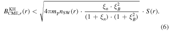
KHI has been observed primarily in EUV observations from SDO/AIA at low-corona distances during the early stages of CME formation (Foullon et al. 2011; Ofman & Thompson 2011; Möstl et al. 2013). Páez et al. (2017) discussed the possibility of KHI formation in the mid and outer corona, in particular at heliocentric distances between 4 and 30 R⊙. In our work, we assess the possibility that WISPR actually observed a KHI in the wake of a CME, in particular, near its southern flank, at heliocentric distances between 7.5 and 9.5 R⊙.
In our approach, we consider the case where the wavevector,  , is parallel to the flows, namely to both the CME and the ambient solar wind, which can be stabilized by the flow-aligned magnetic field. For our case, we need to study the magnetic field and density environment along the shear flow, for an incompressible plasma without viscosity and in a thin layer with an external magnetic field. Therefore, to evaluate where a KHI can develop, we utilize the KHI magnetic condition as proposed in Michael (1955) and Chandrasekhar (1961):

where
V
1 and
V
2 are the velocities, n1 and n2 are the number densities,
B
1 and
B
2 are the magnetic fields of the two magnetized plasma flows, mp is the proton mass, and  is the wavevector of the shear flow. Equation (1) represents the condition that is necessary for the development of the KHI in the boundary layer between the two flows, considering that the thickness of the boundary layer is negligible (i.e., Δ = 0), as long as the left-hand side is greater than the right-hand side.
In the following, we investigate the constraints on the 2021 November 19 CME magnetic field as a function of distance from the Sun that are required to create favorable conditions for the formation of a KHI. To this aim, we follow a similar methodology as in Páez et al. (2017).
The 2021 November 19 CME was a slow event, slower than the ambient solar wind, and as a result, no shock or sheath region around the CME was observed (Howard et al. 2022). In Figure 6, we present a cartoon with a simplified view of the CME and the fast ambient solar-wind environment (top panel), and the magnetic configuration of the KHI on the CME flanks (lower panel). In particular, in the lower panel, we display a vertical cut of the helical magnetic field structure of the CME where the dark blue arrows represent the outward and inward magnetic field polarities on the plane of the image. For our case study, in the region between the CME flanks and the ambient solar wind, Equation (1) becomes:
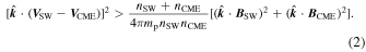

Figure 6. Top panel: 2D cartoon of the CME propagating in the solar wind. The candidate region favorable for the development of the KHI is at the flank of the CME. The dark blue outward arrows with dotted gray inward lines represent the helical magnetic structure of the CME, enveloped by the ambient solar-wind magnetic field (blue lines). The magenta arrow depicts the toroidal magnetic field. The direction of the shear flow close to the CME flanks is indicated with the vector  . Lower panel: zoom-in of the region to detail the magnetic configuration. The helical magnetic field structure of the CME is represented with dark blue arrows for the outward polarity starting from the lower of the orange rectangular box (indicating a part of the CME close to the flank) and ending in the top part of the box between the symbols ⊙ and ⨂. The gray dashed arrows depict the inward polarity. The CME's magnetic field
B
CME is decomposed into a poloidal (
. Lower panel: zoom-in of the region to detail the magnetic configuration. The helical magnetic field structure of the CME is represented with dark blue arrows for the outward polarity starting from the lower of the orange rectangular box (indicating a part of the CME close to the flank) and ending in the top part of the box between the symbols ⊙ and ⨂. The gray dashed arrows depict the inward polarity. The CME's magnetic field
B
CME is decomposed into a poloidal ( , in red) and a toroidal (
 , in magenta) component. The ambient solar-wind magnetic field
B
SW is represented with the blue color lines.
, in magenta) component. The ambient solar-wind magnetic field
B
SW is represented with the blue color lines.
Download figure:
Standard image High-resolution imageThe term  on the right-hand side of Equation (2) can be decomposed in two terms to account for the poloidal,
  , and toroidal,
  , components of the CME magnetic field, i.e.,:

As shown in Figure 6 (lower panel),  is perpendicular to the shear flow
  . Therefore, this term is zero, and hence it does not affect the formation of the KHI (Chandrasekhar 1961). On the other hand, since
  is parallel to
  , the term
  is the relevant one for the formation of the KHI. Then, we can take this radial component equal to the CME radial magnetic field, i.e.,

Since both
V
SW and
V
CME are parallel to  , the left side of Equation (2) can be defined as a shear function, S(r):

S(r) represents the shear flow between the CME and the ambient solar wind. In our case, the solar-wind speed, as estimated from a solar-wind tracer, was assumed to be constant (∼410 km s−1, see Section 3.2.1). On the other hand, the CME speed, as estimated from two particular features of the bulk of the CME (features A and B in Figure 1; see Section 3.1) was found to exhibit a slight acceleration trend during its development, varying from ∼175 km s−1 at a distance of 5 R⊙ up to ∼290 km s−1 at 25 R⊙.
With the above constraints, we can transform Equation (2) into a parametric form. To that aim, as we do not know the actual values of the magnetic field and density of both the CME and ambient solar wind, we define the ratios ξn
=  and
and  . Here, the solar-wind magnetic field is all in the radial direction, so, BSW,r
= BSW. Using these ratios in Equation (2) and solving it for BCME,r
, we obtain the parametric form:
. Here, the solar-wind magnetic field is all in the radial direction, so, BSW,r
= BSW. Using these ratios in Equation (2) and solving it for BCME,r
, we obtain the parametric form:
Equation (6) shows that by just expressing the unknown CME field and density values in units of the solar-wind counterparts, we can estimate the magnetic field values of the CME,  , that might be favorable for the development of a KHI. In particular, we note that
  depends on (1) the density of the ambient solar wind, nSW(r); (2) the shear flow function, S(r); and (3) the CME relative magnetic field strength and density with respect to those of the solar wind, ξB
and ξn
. To estimate the density of the ambient solar wind, nSW(r), we use the Leblanc density model (Leblanc et al. 1998):
depends on (1) the density of the ambient solar wind, nSW(r); (2) the shear flow function, S(r); and (3) the CME relative magnetic field strength and density with respect to those of the solar wind, ξB
and ξn
. To estimate the density of the ambient solar wind, nSW(r), we use the Leblanc density model (Leblanc et al. 1998):
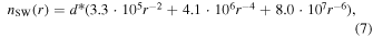
where d is the scaling factor. The scaling factor is used to normalize the Leblanc density model to the instantaneous value of the in situ density measurement obtained from the Advanced Composition Explorer Solar Wind Electron, Proton, and Alpha Monitor (ACE SWEPAM; McComas et al. 1998) instrument. This allowed us to approximate the density value close to the Sun following Thernisien & Howard (2006). Since the CME event was associated with a streamer blowout, we scale the model as in Thernisien & Howard (2006; i.e., d = 6.0). The values resulting from this approach are within the density range estimated from several electron density models close to a coronal streamer (see, e.g., Figure 1 in Raouafi 2011 and references therein).
The CME observed is denser than the ambient solar wind (nCME > nSW). Hence, for the following parametric analysis, we assume ξn
= 2 (this choice is discussed in Section 4), and ξB
= j, with j = 1, 2, 3, q (q ≫ 1). Note that with ξB
= 1 (ξB
= q), we are assuming that the CME has a magnetic field similar to (much larger than) that of the solar wind. This represents a lower (upper) limit, for the ξn
= 2 scenario, hence constraining the range of possible  . In the top panel of Figure 7, we plot the output of the parametric analysis (Equation (6)) for the cases mentioned above and the density model considered. The continuous lines delineate
  at the limit cases when the two sides of Equation (6) are equal. For comparison, we also plot with the dashed, magenta line the CME magnetic radial evolution assuming a power-law curve of the form Br
∝ 1/r2 (see, e.g., Patsourakos & Georgoulis 2016, and references therein) from a PSP/FIELDS in situ measurement of the radial component of the magnetic field (∼550 nT, magenta star) when PSP was at ∼14.1 R⊙ and intersected with the leg of the CME (November 20 23:00–November 21 01:00, McComas et al. 2023). It must be noted that this in situ magnetic field measurement was not taken at the time/location when/where the eddies were observed but rather one day later. This estimate of the CME magnetic field at lower coronal heights is a valid approach. However, it should not be regarded as the actual magnetic field of the CME at the boundary layer where the eddies were observed. We also include two cases representative of different scenarios: the very simple case assuming ξn
= ξB
=1 (light green line) and the extreme case where ξn
= ξB
=q, with q ≫1 (light blue line). These two cases serve as the boundaries of our analysis, representing the lower and upper limits of the outputs from Equation (6). The area delimited by the two vertical, blue dashed lines depicts the distance range where the train of eddies was observed, i.e., between 7.5 R⊙ and 9.5 R⊙. Therefore, the graded, shaded area (ξB
>1) indicates the range of
at the limit cases when the two sides of Equation (6) are equal. For comparison, we also plot with the dashed, magenta line the CME magnetic radial evolution assuming a power-law curve of the form Br
∝ 1/r2 (see, e.g., Patsourakos & Georgoulis 2016, and references therein) from a PSP/FIELDS in situ measurement of the radial component of the magnetic field (∼550 nT, magenta star) when PSP was at ∼14.1 R⊙ and intersected with the leg of the CME (November 20 23:00–November 21 01:00, McComas et al. 2023). It must be noted that this in situ magnetic field measurement was not taken at the time/location when/where the eddies were observed but rather one day later. This estimate of the CME magnetic field at lower coronal heights is a valid approach. However, it should not be regarded as the actual magnetic field of the CME at the boundary layer where the eddies were observed. We also include two cases representative of different scenarios: the very simple case assuming ξn
= ξB
=1 (light green line) and the extreme case where ξn
= ξB
=q, with q ≫1 (light blue line). These two cases serve as the boundaries of our analysis, representing the lower and upper limits of the outputs from Equation (6). The area delimited by the two vertical, blue dashed lines depicts the distance range where the train of eddies was observed, i.e., between 7.5 R⊙ and 9.5 R⊙. Therefore, the graded, shaded area (ξB
>1) indicates the range of  values that support our hypothesis (i.e., that the train of eddies observed is a signature of a KHI instability). The graph shows, in brief, that the assumptions taken lead to a case that can explain the occurrence of the KHI. In fact, the top panel of Figure 7 clearly indicates an increase in instability with larger radii. At 5 R⊙, the magenta dashed curve is positioned above all unstable curves, indicating stability under every tested condition. However, at 25 R⊙, it is situated below all curves except for ξn
= ξB
= 1, signifying instability under all conditions except that one.
values that support our hypothesis (i.e., that the train of eddies observed is a signature of a KHI instability). The graph shows, in brief, that the assumptions taken lead to a case that can explain the occurrence of the KHI. In fact, the top panel of Figure 7 clearly indicates an increase in instability with larger radii. At 5 R⊙, the magenta dashed curve is positioned above all unstable curves, indicating stability under every tested condition. However, at 25 R⊙, it is situated below all curves except for ξn
= ξB
= 1, signifying instability under all conditions except that one.

Figure 7. CME magnetic field constraints for the development of KHI (Equation (6)). Top panel: assuming a scaling factor d in the Leblanc density model (Equation (7)) as in Thernisien & Howard (2006; i.e., d = 6.0). Lower panel: assuming d ≈ 0.5 to match the in situ PSP/SWEAP (Kasper et al. 2016) density measurements when PSP crossed the leg of the CME (S/C at ∼14.1 R☉, between November 20 23:00 UT and November 21 01:00 UT). The colored, continuous lines delineate Equation (6) when both sides are equal for  and
and  (q ≫ 1). The magenta star depicts the magnetic field value measured by the PSP/FIELDS (Bale et al. 2016) when PSP crossed the leg of the CME and the dashed, magenta line the 1/r2 extrapolation. The shaded, blue area depicts the range of plausible
  in the heliocentric range where the train of eddies was observed.
Download figure:
Standard image High-resolution imageTo put our result in context, in the lower panel of Figure 7 (same color and labeling code), we display the output of the parametric analysis considering the Leblanc density model scaled by d = 0.54 to match the in situ density values measured by PSP one day later at ∼14.1 R⊙. In this case, the graph shows that, with this scaling of the density model, the conditions would not be favorable for the development of a KHI.
Note that if we rearrange Equation (6) with the magnetic field and density on the same side (and write  and nSW = n), we get the relation between the Alfvén speed and the shear flow function S(r):
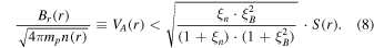
Equation (8) provides another way to examine the favorable conditions for the development of the KHI by comparing the Alfvén speed and the shear flow function S(r) as a function of the ratios ξn and ξB . If we use the PSP in situ measurements at ∼14.1 R⊙ (i.e., Br ∼ 500 nT and n ∼ 950 cm−3) we get an Alfvén speed of about 350 km s−1, which is much higher than the right part of Equation (8). This shows that the formation of a KHI is rather sensitive to local conditions. This explains why we cannot observe the eddies one day later (see Section 4.2).
According to McComas et al. (2023), PSP crossed the leg of the CME between November 20, 23:00 UT and November 21, 01:00 UT, i.e., for a period of about 2 hr. PSP in situ measurements of the electron density by the Solar Wind Electrons Alphas and Protons (SWEAP) Investigation (Kasper et al. 2016) before this interaction averaged a number density of ∼950 cm−3. Inside the CME, the density amounted to ∼ 1800 cm−3 (i.e., ξn ≈ 2). Note that the PSP measurements were obtained at a distance of ∼14.1 R⊙, almost a day after the observations of the eddies; therefore, they can be considered only as a rough estimate of the density conditions at the location of the eddies.
Among other cases, in Figure 7, we plotted Equation (6) for various ξB considering ξn = 2. In particular, we explored the CME magnetic field constraints for the development of KHI assuming a scaling factor in the Leblanc density model as in Thernisien & Howard (2006; i.e., d = 6.0; Figure 7 top panel). Next, we considered a scaling factor d ≈ 0.5 to match the in situ PSP/SWEAP density measurements when PSP crossed the CME leg (Figure 7 lower panel). Now, we explore the case when the density model is scaled such that the in situ PSP/FIELDS measurements of the CME magnetic field match the magnetic field constraints from Equation (6). The average in situ PSP/FIELDS values of the magnetic field before the interaction of PSP and the CME was ∼500 nT, and slightly higher at ∼550 nT while inside the CME. By considering this approach, we are assuming that the in situ PSP measurements of the magnetic field (although they were taken one day later in a region of space far away from the eddies location), serve as a ground truth. Note, however, that, while this assumption is speculative and not representative of the conditions where the eddies were observed (see also Section 3.3), it might represent a plausible approximation. These two values of the magnetic field indicate ξB ≈ 1 while ξn = 2 (this set is represented by the red line in Figure 7). We extrapolated them to shorter distances assuming flux conservation, resulting in values 1915/1190 nT of the magnetic field in the distance range where the eddies were observed at 7.5/9.5 R⊙, respectively. To infer the minimum density required for instability under these conditions, the Leblanc density model must be scaled accordingly so that this red line matches the extrapolated magnetic field of the CME (i.e., the magenta dashed) at the distance where the eddies were observed (i.e., between the vertical blue dashed lines). To achieve this, the scaling factor becomes d ∼ 14.6. This new case is illustrated in Figure 8. From our approach, considering ξn = 2 and ξB = 1, we have that the KHI criterion is satisfied for CME magnetic fields less than 1915/1350 nT at 7.5/9.5 R⊙, respectively. The newly scaled density model results in very high density values, so we shed light on this fact by comparing it to instances of high density values recorded by PSP. For example, the highest density measured by PSP up to Orbit 15 (as obtained using the simplified quasi-thermal noise spectroscopic technique or SQTN; Moncuquet et al. 2020) was ∼2.13 · 104 cm−3. This measurement occurred on 2022 June 2 at approximately 14:10 UT when the S/C was at ∼15.8 R⊙. This case is considered here as a special case and definitely not assumed as typical of a background solar wind. The newly scaled density model (d ∼ 14.6) predicts, at the corresponding distance, a density value of ∼2.0 · 104 cm−3, which is a comparable estimate (∼7% lower) and certainly is not a nonphysical estimate. As the CME under study was associated with a streamer blowout, we expect that the compression of the already dense plasma from the streamer becomes denser as the CME develops. Consequently, this results in a higher local density, favoring the formation of a KHI.

Figure 8. CME magnetic field constraints for the development of KHI (Equation (6)). Same as in Figure 7 for a Leblanc density model with scaling factor d ∼ 14.6 chosen to match the extrapolated magnetic field of the CME at 7.5 R☉ where the eddies were observed. Note that the extrapolated magnetic field values (magenta dashed curve) are positioned below the most probable unstable case with ξn = 2 and ξB = 1 (red curve) indicating that is favorable for the development of the KHI. For details, see the text.
Download figure:
Standard image High-resolution image4. Discussion
4.1. Theoretical Support for the KHI Interpretation
In this work, we investigate the possibility that a train of small vortex-like structures, detected in the aftermath of a CME, are the signatures of Kelvin–Helmholtz instability. To assess the likelihood of such a physical phenomenon, we compare the measured dynamical and kinematic properties of the eddies against theoretical expectations under certain assumptions.
The relative distance between the centroids of the vortexes is considered to be the characteristic length scale for the associated projected wavelength, or spatial period λ. In many KHI simulations or observations in solar coronal physics, the wavelength estimates are on the order of a few megameters. In particular, Foullon et al. (2011) reported a projected wavelength of λ = 18 ± 0.4 Mm. Möstl et al. (2013) mentioned that the vortex-like structures, which were observed at the northern side of the embedded filament boundary of the 2011 February 24 CME, had a wavelength of approximately λ ∼14.4 Mm. Ofman & Thompson (2011) reported a wavelength of λ = 7 Mm based on the size of the initial ripples. Li et al. (2018) observed a KHI in a solar blowout jet with a λ ∼5 Mm. All of the aforementioned studies estimated the wavelength based on EUV observations at low coronal heights (< 160 Mm). Kieokaew et al. (2021) reported a KHI analysis based on in situ measurements from Solar Orbiter. Their wavelength estimates, λ = 66.4 ± 8.4 Mm, are larger than the coronal one. We estimate a wavelength average of λ = 237.5 (58.6) Mm based on the distances between the eddies (Table 2).
A key discriminant for a KHI is the wavelength of the fastest growing mode. The fastest growing mode excited by a KHI at the interface should have a spatial period, or wavelength λ, between 2πΔ and 4πΔ (Miura & Pritchett 1982), where Δ is the thickness of the boundary layer. Equation (6) was obtained under the assumption of a boundary layer of zero thickness. We can now relax this assumption. From the WISPR-I images, we can estimate both Δ and λ independently. If the eddies are signatures of KHI, they should satisfy the relation 2πΔ < λ < 4πΔ. If not, then the eddies are not a KHI signature. In general, it is challenging to estimate Δ from imaging observations due to the small scales involved. Thanks to the proximity to the CME, WISPR-I resolves many small-scale details. In particular, at 02:48:20 UT all the vortexes are fully deformed, creating a thin line of plasma (Figure 4, panel (F)). We take the width of this line, Δobs = 28 (7) Mm as the upper limit of the boundary layer thickness. Therefore the wavelength of the fastest growing mode should lie between 2πΔ = 176 Mm and 4πΔ = 352 Mm. From the observations, we estimate λ as the relative distance between the vortexes (169–306 Mm, see also Table 2), with an average value of 237.5 Mm. Thus, the observed λ satisfies the condition of the fastest growing KH mode for most cases, which, in turn, supports our hypothesis that the observed eddies are the results of the development of a KHI.
Another physical parameter to check for the plausibility of a KHI is the growth rate. The linear growth rate of a KHI in incompressible, inviscid fluid layers with equal density, equal field strength, separated discontinuously within a "vortex sheet" (Chandrasekhar 1961; Frank et al. 1996), associated with, and which leads to, the KHI criterion (Equation (1)), is given by:

where the k is the wavevector whose magnitude is equal to 2π/λ, Δ V is the velocity difference between the two layers (i.e., the shear flow function S(r) defined in Equation (5)) and VA is the Alfvén speed (see Equation (8)). In the case of an interface region with finite thickness, the growth rate is even smaller than the predicted value according to Equation (9) (see, e.g., Miura & Pritchett 1982; Ofman & Thompson 2011). Compressible plasma also tends to reduce the growth of the instability. Based on the parameters we estimated before we can compute the upper and lower limit values of the linear growth rate of the KHI using Equation (9). If we use an Alfvén speed range between 20 and 65 km s−1 (see Section 4.2 for details), k = 2π/λ with λ the average value of 237.5 Mm, and ΔV ∼200 km s−1, we get, from Equation (9), upper and lower γKH values of 0.0027 and 0.0022 s−1, respectively. If we assume that nonlinear saturation occurs on a timescale of a few γ−1 (see, e.g., Kieokaew et al. 2021), which ranges in our case from ∼6.1 to 7.6 minutes, the observed timescale evolution of the eddies recorded in WISPR-I images (less than 30 minutes) falls within the expected values. Table 3 compares various KHI parameters from past works against the estimates described in this section.
Table 3. Comparison of Critical Parameters Estimates on Selected Observations of KHI among Different Works Including Ours
| Publication | Observations | Wavelength λ | Thickness Δ | Growth Rate γ | Heliocentric Distance |
|---|---|---|---|---|---|
| (Mm) | (Mm) | (s−1) | (R⊙) | ||
| Foullon et al. (2013) | EUV a | 18.5 | 4.1 | 0.033 | < 1.22 |
| Möstl et al. (2013) | EUV a | 14.4 | 1–2 | ⋯ | ⋯ |
| Ofman & Thompson (2011) | EUV a | 7 | 0.4 | 0.003–0.009 | ⋯ |
| Li et al. (2018) | EUV b | 5 | 0.5 | 0.063 | ⋯ |
| Kieokaew et al. (2021) | in situ c | 66.4 | 5.3–10.5 | 0.0015 | 148.3 |
| This work | White Light d | 237.5 | 28 | 0.0022–0.0027 | 7.5–9.5 |
Notes.
a [SDO/AIA]. b [IRIS]. c [Solar Orbiter/MAG,SWA]. d [PSP/WISPR-I].Download table as: ASCIITypeset image
4.2. Modeling Support for the KHI Interpretation
According to Equation (8), the formation of a KHI is possible if ΔV >2 · VA (Miura & Pritchett 1982), where ΔV is the shear flow function S(r) (Equation (5)) and VA is the Alfvén speed (Equation (8)), assuming equal densities (i.e., ξn
= 1) and magnetic fields (i.e., ξB
= 1). With existing instrumentation, it is impossible to measure the actual density and magnetic field, and by extension VA
, at the heliocentric distances where the plausible KHI was observed (7.5 R⊙–9.5 R⊙). Since we know S(r) for this region (lower panel of Figure 3), we can, provide an upper limit on VA <  S(r)∼100 km s−1 for the onset of a plausible KHI. This value appears to be low for such heliocentric distances, especially for a CME-related feature. However, we note that this speed corresponds to the component parallel to the flow. It is conceivable that the Alfvén speed perpendicular to the flow is much higher, leading to a higher overall VA. An obvious scenario would be the propagation of a curved magnetic structure in a parallel flow. Figure 1 (and the movie available on the web at the WISPR home page) indicate that the structures surrounding the area of interest are indeed curved as they seem to form the lower extensions of the helical structures comprising the CME magnetic flux rope.
An alternative way to explore the constraints of the Alfvén speed is to use the output of a model for this specific date. To that aim, we utilize the thermodynamic MHD code "Magnetohydrodynamic Algorithm outside a Sphere" (MAS), which was developed by and is maintained at Predictive Science Inc. (see, e.g., Riley et al. 2012, and references therein). The VA as estimated with the MAS model for Carrington rotation 2251 at a distance of 8.43 R⊙ (i.e., at a distance within the distance range where the eddies were observed) is displayed in the top panel of Figure 9. The propagation direction of the CME on 2021 November 20 at ∼02:00 UT (i.e., during the time of the eddies) as estimated with the GCS model (Carrington longitude and latitude of 20° and 10°, respectively; Section 3.1) is indicated with the magenta star symbol. We notice in the figure that VA for the ambient solar wind near the CME is <30 km s−1. The propagation direction of the CME is almost above the location of the heliospheric current sheet (HCS) and as a result, the very low Alfvén speeds at these positions are reasonable. This result provides another supporting evidence for our hypothesis.

Figure 9. Top panel: Alfvén speed, VA, on a Carrington projection (rotation 2251) from the MAS model at 8.43 R⊙. The propagation direction of the CME on 2021 November 20 at 02:00 UT is pointed out with the magenta star symbol (i.e., about the time the eddies were observed). This direction is very close to the heliospheric current sheet (delineated with the white line). The local Alfvén speeds in this area are very low (of the order of 30 km s−1). Lower panel: VA radial profiles from the MAS model for the Carrington longitude and latitude of the CME considering a 2° (in light blue) and a 5° (in gray) error. The red line represents the radial profile considering the CME direction of propagation, and the dashed green line represents the limit condition VA =  S(r) for ξn
= 2 and ξB
= 1 (Equation (8)). The magenta line depicts VA assuming ξn
= ξB
=1 (as in Miura & Pritchett 1982). The black star symbol represents the Alfvén speed calculated using the extrapolated magnetic field values Br
(magenta dashed line in Figure 8). The blue dashed vertical lines indicate the distance range where the eddies were observed (7.5 R⊙–9.5 R⊙).
S(r) for ξn
= 2 and ξB
= 1 (Equation (8)). The magenta line depicts VA assuming ξn
= ξB
=1 (as in Miura & Pritchett 1982). The black star symbol represents the Alfvén speed calculated using the extrapolated magnetic field values Br
(magenta dashed line in Figure 8). The blue dashed vertical lines indicate the distance range where the eddies were observed (7.5 R⊙–9.5 R⊙).
Download figure:
Standard image High-resolution image
Recently, Verbeke et al. (2023) showed that the error in determining the longitude and latitude of a CME direction using the GCS model when two or three viewpoints is approximately 2°. Thus, to assess the effect of our estimate of the CME direction, we consider this error in the lower panel of Figure 9. For all the combinations of these two coordinates available, we created the VA radial profiles for the ambient solar wind, which we display in the lower panel of Figure 9 with the light blue lines. In this case, VA is ⪅75 km s−1 at 7.5 R⊙ and ⪅55 km s−1 at 9.5 R⊙. For a more ample case, we also assumed ad hoc a larger error (5°, represented by the gray lines). The red line represents the radial profile considering the direction of propagation of the CME, and the dashed green line represents the limit condition VA =  S(r) for ξn
= 2 and ξB
= 1 (Equation (8)). The magenta curve represents the VA assuming ξn
= ξB
=1 (as in Miura & Pritchett 1982). The black star symbol represents the Alfvén speed calculated using the extrapolated magnetic field Br
and density values similar to the values used in Figure 8. We note that, in the range where the eddies are observed (delimited by the dashed blue lines), all the VA radial profiles satisfy Equation (8), regardless of the error, and hence support our hypothesis.
S(r) for ξn
= 2 and ξB
= 1 (Equation (8)). The magenta curve represents the VA assuming ξn
= ξB
=1 (as in Miura & Pritchett 1982). The black star symbol represents the Alfvén speed calculated using the extrapolated magnetic field Br
and density values similar to the values used in Figure 8. We note that, in the range where the eddies are observed (delimited by the dashed blue lines), all the VA radial profiles satisfy Equation (8), regardless of the error, and hence support our hypothesis.
This condition perhaps offers an indication of why KHI observations are rare at these heights. From our analysis, it becomes clear that the development of a KHI (and its observation in white light) requires a combination of conditions to be in place:
- 1.two flows with varying speeds;
- 2.an unusually low Alfvén speed or an interaction geometry leading to a weak parallel and strong perpendicular VA components relative to the flow to satisfy the Equation (8);
- 3.short LOS imaging observations to resolve small scales (PSP is the only platform capable of providing this vantage point so far; therefore, it is unsurprising that white-light signatures of KHI have not been detected before).
- 4.favorable viewing conditions, in addition to short LOS. The location of PSP below the CME plane offered a favorable viewing angle for observing the complex CME structure across a wide longitude and further avoiding LOS overlap. Furthermore, PSP was transiting over a coronal hole region at the time, and hence the WISPR-I LOS was crossing through a partially depleted region, resulting in a "cleaner" LOS. Stenborg et al. (2023) recently showed that the presence of even small equatorial Coronal Holes (CHs) can directly affect the overall brightness observed by WISPR-I. This is another argument in support of the assumption that the ambient solar wind below the CME has a larger speed than the CME.
As a final thought, the 2021 November 19 CME was associated with a streamer blowout (Howard et al. 2022), and originated in a quiet-Sun region. Therefore, it must have had lower magnetic field strengths than CMEs associated with active regions (Vourlidas & Webb 2018). Thus, the weak magnetic obstacle in combination with the orientation of the magnetic field could have been favorable for the formation of a KHI.
5. Summary and Conclusions
In this paper, we examined the possibility that a train of small-scale features observed by WISPR-I was the signature of a KHI. To test this hypothesis, we performed a comprehensive theoretical and observational analysis. Candidate KHI features were observed along the southern flank of a CME between 7.5 R⊙ and 9.5 R⊙ and lasted about 30 minutes. The kinematic analysis of the CME indicated a slow event, most likely associated with a streamer blowout, developing with a (deprojected) speed of ∼200 km s−1. By measuring the speed of solar-wind tracers, we estimated the speed of the ambient solar wind to be ∼410 km s−1. On the basis of KHI theoretical considerations, we investigated the magnetic field conditions and estimated the values favorable for the development of a KHI under certain assumptions. We found that a KHI interpretation is reasonable under certain conditions. For instance, assuming that the extrapolated values of the magnetic field values recorded by PSP/FIELDS at 14.1 R⊙ are a reasonable choice at lower heights, then the KHI occurs
- 1.
- 2.if the magnetic field strength of the CME is larger than that of the ambient solar wind (i.e., ξB > 1; all cases in Figure 8).
In both cases, high local densities are required (Leblanc model scaled by a factor of d ∼ 14.6). On the other hand, if we ignore the constraint imposed by the magnetic field measurements at 14.1 R⊙, and simply assume a Leblanc model scaled by a factor that can be considered typical of a streamer (d = 6), then the KHI occurs for various combinations of ξB and ξn (Figure 7, top panel). 7
Furthermore, we used the MAS model to estimate the Alfvén speed, VA, in the distance range where the eddies were observed. In all the cases considered (Figure 9) the modeled VA satisfies the criterion for the development of the KHI (Equation (8)).
We also measured the longitudinal and transverse size of the vortex-like features via a technique that offers an objective estimation. From these measurements, we showed that the eddies increased in size while maintaining a relatively constant separation distance. These characteristics are consistent with the evolution of Kelvin–Helmholtz vortexes and hence are in support of our hypothesis.
To further evaluate our interpretation, we used the following approach. First, we measured the thickness of the boundary layer along which the KHI candidate signatures were observed (∼28 Mm). This is probably an upper limit to the true thickness. Then, we consider that the wavelength, λ, of the fastest growing mode at the interface should lie between 2πΔ and 4πΔ (Miura & Pritchett 1982). In fact, we found that λ lies between 176 and 352 Mm and these values are in agreement with the relative distances between the eddies we measured in WISPR-I images. These two independent quantities, measured using WISPR-I images, satisfy the relation 2πΔ < λ < 4πΔ (Miura & Pritchett 1982), thereby supporting our hypothesis that the observed eddies are signatures of KHI.
Assuming equal densities and magnetic fields (i.e., ξn = 1 and ξB = 1), we estimated a linear growth rate of the KHI, γ, between ∼0.0022 and ∼0.0027 s−1. Since nonlinear saturation occurs within a few γ−1, this also determines the lifetime of KHI. The WISPR features lasted ∼30 minutes, which corresponds to about 6γ − 8γ and hence is consistent with the KHI interpretation.
The comparisons between theoretical expectations and observational estimates of the properties of these vortex-like features lead us to conclude that they are consistent with KHIs. This marks the first direct imaging of such plasma phenomena in the middle corona (r < 15 R⊙). If it is verified with additional detections and theoretical/modeling analysis, it will open a new observing window into coronal plasma dynamics. The study of plasma instabilities may help understand the role of viscosity in CME development and propagation. Finally, the dimensions of the KHI, as presented in our study, coupled with the intricate structures discerned within CMEs in WISPR images, underscore the significance of further investigation into mesoscale structures (a few tens to 2000–3000 Mm). However, such observations are likely exceedingly rare given the requirement of appropriate physical conditions, i.e., the observer's proximity to the region, favorable viewing conditions, the topology and orientation of the local magnetic fields, and the necessary combination of the densities and speeds of the different flows. On the other hand, PSP/WISPR offers a unique, possibly the only, means to image such events especially as the PSP continues to approach closer to the Sun.
Acknowledgments
The authors thank A. Kouloumvakos and V. Jagarlamudi for useful discussions. E.P. was supported by NASA grant 80NSSC19K0069. G.S., A.V., and R.H. were supported by WISPR Phase E funds and NASA grant 80NSSC22K0970. M.G.L. was supported by WISPR Phase E funds under NASA grant NNG11EK11I and by the NASA Living with a Star Focused Science Topic program NNH21ZDA001NLWS "The Origin of the Photospheric Magnetic Field: Mapping Currents in the Chromosphere and Corona" (PI P. Schuck). Parker Solar Probe was designed, built, and is now operated by the Johns Hopkins Applied Physics Laboratory as part of NASA's Living with a Star (LWS) program (contract NNN06AA01C). Support from the LWS management and technical team has played a critical role in the success of the Parker Solar Probe mission. The Wide-Field Imager for Parker Solar Probe (WISPR) instrument was designed, built, and is now operated by the U.S. Naval Research Laboratory in collaboration with JHU Applied Physics Laboratory, California Institute of Technology/Jet Propulsion Laboratory, University of Goettingen, Germany, Centre Spatiale de Liege, Belgium, and University of Toulouse/Research Institute in Astrophysics and Planetology. The STEREO SECCHI data are produced by a consortium of RAL (UK), NRL (USA), LMSAL (USA), GSFC (USA), MPS (Germany), CSL (Belgium), IOTA (France), and IAS (France). The FIELDS instrument suite was designed and built and is operated by a consortium of institutions including the University of California, Berkeley, University of Minnesota, University of Colorado, Boulder, NASA/GSFC, CNRS/LPC2E, University of New Hampshire, University of Maryland, UCLA, IFRU, Observatoire de Meudon, Imperial College and Queen Mary University, London. The SWEAP Investigation is a multi-institution project led by the Smithsonian Astrophysical Observatory in Cambridge, Massachusetts. Other members of the SWEAP team come from the University of Michigan, University of California, Berkeley Space Sciences Laboratory, the NASA Marshall Space Flight Center, the University of Alabama Huntsville, the Massachusetts Institute of Technology, Los Alamos National Laboratory, Draper Laboratory, JHU Applied Physics Laboratory, and NASA Goddard Space Flight Center.
Footnotes
- 4
From the GCS modeling, the CME exhibited an aspect ratio, κ, of ∼0.18; and a half angle, α, of ∼8° (for a detailed description of the GCS parameters see Thernisien 2011).
- 5
The wavelet-processed ST-A/EUVI images for the whole STEREO mission are available at http://sd-www.jhuapl.edu/secchi/wavelets/.
- 6
Magnetic field ⪅1915/1350 nT at 7.5/9.5 R⊙, respectively.
- 7
For example, in the simplest approach of ξB = ξn =1, the KHI occurs for CME magnetic fields ⪅1060/750 nT at 7.5/9.5 R⊙.