


Abstract
One prominent feature in the atmospheres of Jupiter and Saturn is the appearance of large-scale vortices (LSVs). However, the mechanism that sustains these LSVs remains unclear. One possible mechanism is that these LSVs are driven by rotating convection. Here, we present numerical simulation results on a rapidly rotating Rayleigh–Bénard convection at a small Prandtl number Pr = 0.1 (close to the turbulent Prandtl numbers of Jupiter and Saturn). We identified four flow regimes in our simulation: multiple small vortices, a coexisting large-scale cyclone and anticyclone, large-scale cyclone, and turbulence. The formation of LSVs requires that two conditions be satisfied: the vertical Reynolds number is large ( ), and the Rossby number is small (Ro ≤ 0.4). A large-scale cyclone first appears when Ro decreases to be smaller than 0.4. When Ro further decreases to be smaller than 0.1, a coexisting large-scale cyclone and anticyclone emerges. We have studied the heat transfer in rapidly rotating convection. The result reveals that the heat transfer is more efficient in the anticyclonic region than in the cyclonic region. Besides, we find that the 2D effect increases and the 3D effect decreases in transporting convective flux as the rotation rate increases. We find that aspect ratio has an effect on the critical Rossby number in the emergence of LSVs. Our results provide helpful insights into understanding the dynamics of LSVs in gas giants.
Export citation and abstract BibTeX RIS
1. Introduction
Rotation plays an important role in stellar and planetary turbulent convection. It has been observed that long-lived large-scale vortices (LSVs) are formed in rapidly rotating giant planets in our solar system. At the atmosphere of Jupiter, for example, a large-scale Great Red Spot has been observed for more than 180 yr. Recently, large-scale collective cyclones have been observed in polar regions of Jupiter by the Juno spacecraft (Adriani et al. 2018, 2020; Tabataba-Vakili et al. 2020). Despite collective cyclones, dipole configurations of a large-scale cyclone and anticyclone have also been observed in the polar regions of Jupiter (Adriani et al. 2020). For Saturn, Godfrey (1988) reported that a large-scale hexagonal cyclone has been observed in the north pole by the Cassini spacecraft. Later, Vasavada et al. (2006) reported that a large-scale cyclone also exists in the south pole of Saturn. Apart from polar vortices, various cyclones and anticyclones were observed in other regions of Jupiter (Li et al. 2004) and Saturn (Sayanagi et al. 2013). However, the driving mechanism of these vortices remains unclear. There are two scenarios for the explanations: one is based on shallow models (Zhang 2014; O'Neill et al. 2016; Brueshaber et al. 2019), which explain that these vortices can be formed by merging of random storms generated by moist convection; and the other is based on deep models (Chan & Mayr 2013; Yadav & Bloxham 2020; Cai et al. 2021), which explain that these vortices are generated from rotating turbulent convection powered by internal heat. Progress has been made on both types of models recently. For example, based on a shallow model, Brueshaber et al. (2019) searched the parameter space and found that the Burger number (square of the ratio of the Rossby deformation radius to planetary radius) is a key factor in determining the pattern of polar vortices. On the other hand, based on a deep model Cai et al. (2021) has successfully replicated the pentagonal and hexagonal patterns of circumpolar vortices observed on the south pole of Jupiter. It indicates that rapidly rotating turbulent convection might be an important mechanism in generating vortices in gas giant planets. Apart from gas giant planets, LSVs are possibly also prominent features in rapidly rotating stars. LSV-like star spots in cool stars have been observed in stellar atmospheres in Doppler imaging maps (Hackman et al. 2019; Willamo et al. 2019). The star spots observed in cool stars could be associated with the LSVs driven by rotation (Käpylä et al. 2011). In this paper, we will mainly focus on the LSVs formed in rapidly rotating turbulent convection.
Early numerical simulation (Chan 2007) on compressible convection in Cartesian geometry discovered that LSVs could be generated when the rotation is fast. This phenomena has been confirmed in subsequent works on rapidly rotating compressible convection (Käpylä et al. 2011; Mantere et al. 2011; Chan & Mayr 2013; Cai 2016; Cai et al. 2021). For simulations on incompressible flow, LSVs were first reported in Julien et al. (2012) and Rubio et al. (2014), where a set of reduced rapidly rotating Rayleigh–Bénard equations were solved. The appearance of LSVs was also observed in direct numerical simulations on rapidly rotating Rayleigh–Bénard convection (RRBC; Favier et al. 2014; Guervilly et al. 2014, 2015; Kunnen et al. 2016; Guervilly & Hughes 2017; Novi et al. 2019). In these simulations, a large-scale cyclone appears with associated large-scale circulation of small anticyclonic vortices. The flow patterns of a coexisting large-scale cyclone and anticyclone in RRBC were reported when the Rayleigh number achieved 2 × 10¹¹ at Pr = 1 (Stellmach et al. 2014) with a stress-free boundary condition and 1.5 × 10¹¹ at Pr = 5.2 with no-slip boundary condition (Guzmán et al. 2020). In spherical geometry, LSVs were also found recently in an elastic convection (Yadav & Bloxham 2020) and incompressible convection (Lin & Jackson 2021).
So far, most of the studies on RRBC have been focused on the moderate Prandtl number region Pr ∼ O(1). However, the Prandtl numbers in stars or gas giant planets are usually smaller than one (Schubert & Soderlund 2011; Kupka & Muthsam 2017). Linear instability analysis shows that the fluid at small Pr behaves different from that at large Pr (Chandrasekhar 2013; Zhang & Busse 1987). For example, the onset of instability first occurs as oscillatory convection when Pr < 0.67 in the fluid on an infinite planes (Chandrasekhar 2013). The critical Rayleigh number Rac
for the onset of convection is much lower at low Pr ( ) than at high Pr (Rac
∼ 8.7E−4/3) (Chandrasekhar 2013), where E is the Ekman number. In addition, experiments on liquid metal gallium (Pr = 0.025) with and without rotation have shown that the convective behavior of low Pr is substantially different from that of moderate Pr (King & Aurnou 2013). At moderate Pr, four flow regimes are identified: cells, convective Taylor column, plumes, and geostrophic turbulence (Julien et al. 2012). The trend toward lower Pr indicates that geostrophic turbulent regime is approaching at low Pr (Aurnou et al. 2015). Compressible simulations on rapidly rotating convection (Käpylä et al. 2011; Chan & Mayr 2013; Cai 2016) showed that at low Pr the flow favors in the formation of LSVs. Hence, we expect that the flow regimes would be different from those identified in the simulations at moderate Pr. Previous simulations on Rayleigh–Bénard convection at Pr = 0.1 with no-slip boundary condition found large-scale cyclones when the rotation is fast (Guzmán et al. 2020). In this paper, we will explore the flow regimes of RRBC at low Pr with stress-free boundary condition through numerical simulations. We find that the flow pattern of a coexisting large-scale cyclone and anticyclone appears in RRBC. We will also discuss the energy and heat transfer among different regimes.
) than at high Pr (Rac
∼ 8.7E−4/3) (Chandrasekhar 2013), where E is the Ekman number. In addition, experiments on liquid metal gallium (Pr = 0.025) with and without rotation have shown that the convective behavior of low Pr is substantially different from that of moderate Pr (King & Aurnou 2013). At moderate Pr, four flow regimes are identified: cells, convective Taylor column, plumes, and geostrophic turbulence (Julien et al. 2012). The trend toward lower Pr indicates that geostrophic turbulent regime is approaching at low Pr (Aurnou et al. 2015). Compressible simulations on rapidly rotating convection (Käpylä et al. 2011; Chan & Mayr 2013; Cai 2016) showed that at low Pr the flow favors in the formation of LSVs. Hence, we expect that the flow regimes would be different from those identified in the simulations at moderate Pr. Previous simulations on Rayleigh–Bénard convection at Pr = 0.1 with no-slip boundary condition found large-scale cyclones when the rotation is fast (Guzmán et al. 2020). In this paper, we will explore the flow regimes of RRBC at low Pr with stress-free boundary condition through numerical simulations. We find that the flow pattern of a coexisting large-scale cyclone and anticyclone appears in RRBC. We will also discuss the energy and heat transfer among different regimes.
2. The Model
For the RRBC in a Cartesian box, the nondimensional hydrodynamic equations describing mass, momentum, energy conservations can be written as


where
u
is the velocity, p is the reduced pressure,  is the unit vector in the vertical direction, Θ is the superadiabatic temperature, Ts
is the static reference state of the temperature, ν is the kinematic viscosity, κ is the thermometric conductivity, g is the gravitational acceleration, α is the coefficient of volume expansion, H is the height of the box, δ
T is temperature difference between the bottom and top of the box, Ω is the angular velocity, Pr = ν/κ is the Prandtl number, Ra = g
α
δ
TH3/(ν
κ) is the Rayleigh number, E = ν/(2ΩH2) is the Ekman number, and Ro = ReE is the convective Rossby number. We also define the Reynolds number
is the unit vector in the vertical direction, Θ is the superadiabatic temperature, Ts
is the static reference state of the temperature, ν is the kinematic viscosity, κ is the thermometric conductivity, g is the gravitational acceleration, α is the coefficient of volume expansion, H is the height of the box, δ
T is temperature difference between the bottom and top of the box, Ω is the angular velocity, Pr = ν/κ is the Prandtl number, Ra = g
α
δ
TH3/(ν
κ) is the Rayleigh number, E = ν/(2ΩH2) is the Ekman number, and Ro = ReE is the convective Rossby number. We also define the Reynolds number  , and the Péclet number Pe = RePr. In the above equations, the normalizing factors for length, time, velocity, pressure, and superadiabatic temperature are H,
  ,
,  ,
,  , and δ
T, respectively.
, and δ
T, respectively.
To solve the incompressible equations, the velocity is decomposed into

where Φ and Ψ are the poloidal and toroidal potentials. Applying the operators  and
and  to the momentum equation, we have


where the subscript h denotes the horizontal component, Δ is the Laplacian operator,
ω
is the vorticity, and
G
=
ω
×
u
is a nonlinear term. Equations (5)–(7) are solved numerically using a mixed finite-difference pseudo-spectral method. Fourier transforms are applied in the horizontal directions, and a second-order finite-difference method is adopted in the vertical direction. A 2/3 dealiasing rule was used for the pseudo-spectral scheme in the horizontal direction. All the linear terms on the left-hand side of Equations (5)–(7) are integrated by a second-order semi-implicit scheme. The quadratic nonlinear terms on the right-hand side of Equations (5)–(7) are integrated by a third-order explicit Adams–Bashforth scheme. The numerical method is similar to the one developed in Cai (2016), where a compressible flow is considered instead. The upper and lower boundary conditions are taken to be thermally conducting, impenetrable and stress-free. The lateral boundary conditions on both sides are periodic. The grid points on the horizontal directions are uniformly distributed. On the vertical direction, Chebyshev–Gauss–Lobatto grid points are used to resolve the boundary layers. The lateral-to-height aspect ratios are set to be unity (Γ = 1). In this paper, we choose a small fixed Prandtl number Pr = 0.1. Three groups of simulations with different Rayleigh numbers Ra = 106, 107, and 108 are performed. In each group, the reduced Rayleigh numbers  are varied from 1–1000 for comparisons.
  is related to the supercritical Rayleigh number Rac
∼ O(E−4/3) (Chandrasekhar 2013; Julien et al. 2012). For a rotating Bénard flow with Pr > 0.67 in a layer, the onset of instability first occurs as stationary convection when Ra > Rac1 = 8.7E−4/3 (Chandrasekhar 2013). For Pr < 0.67, the onset of instability first occurs as oscillatory convection when
is related to the supercritical Rayleigh number Rac
∼ O(E−4/3) (Chandrasekhar 2013; Julien et al. 2012). For a rotating Bénard flow with Pr > 0.67 in a layer, the onset of instability first occurs as stationary convection when Ra > Rac1 = 8.7E−4/3 (Chandrasekhar 2013). For Pr < 0.67, the onset of instability first occurs as oscillatory convection when  (Chandrasekhar 2013). In this paper, we mainly focus on the small Prandtl number cases at Pr = 0.1, which yields Rac2 = 0.78E−4/3. Since Rac2 is smaller than Rac1 by an order of magnitude, we can explore lower Ekman number regimes with moderate Rayleigh numbers in our simulation. The grid resolutions are Nx
× Ny
× Nz
= 512 × 512 × 257 for the cases with Ra = 108 (group C), and Nx
× Ny
× Nz
= 256 × 256 × 257 for the cases with Ra = 106 (group A) and Ra = 107 (group B). In a low Prandtl flow, the thermal boundary layer is estimated to has a thickness of
(Chandrasekhar 2013). In this paper, we mainly focus on the small Prandtl number cases at Pr = 0.1, which yields Rac2 = 0.78E−4/3. Since Rac2 is smaller than Rac1 by an order of magnitude, we can explore lower Ekman number regimes with moderate Rayleigh numbers in our simulation. The grid resolutions are Nx
× Ny
× Nz
= 512 × 512 × 257 for the cases with Ra = 108 (group C), and Nx
× Ny
× Nz
= 256 × 256 × 257 for the cases with Ra = 106 (group A) and Ra = 107 (group B). In a low Prandtl flow, the thermal boundary layer is estimated to has a thickness of  (Horanyi et al. 1999; King & Aurnou 2013). With a Chebyshev grid distribution in the vertical direction, there are about 40, 30, and 22 grid points within the thermal boundary layers for the cases in groups A, B, and C, respectively. The detailed parameters of simulation cases are shown in Table 1. The critical wavelength ℓc at the onset of convection is also reported for reference. The critical wavelength
 ![${{\ell }}_{c}\approx {2}^{7/6}{\pi }^{2/3}{\left[{\Pr }/(1+{\Pr })\right]}^{-1/3}{E}^{1/3}$](https://content.cld.iop.org/journals/0004-637X/923/2/138/revision1/apjac2c68ieqn14.gif) for a rapidly rotating flow at Pr < 0.67, and ℓc
≈ 27/6
π2/3
E1/3 for a rapidly rotating flow at Pr > 0.67 (Chandrasekhar 2013). In each case, we run the simulation for a long time until the system reaches a statistically thermal relaxation state. In practice, we require that the variation of the averaged Nusselt number (the average is taken temporally and horizontally) is smaller than 1%. The time for reaching statistically relaxation state is different for different cases. For some typical cases, such as C3 and C5, we have run for a period of about 30,000 units of time (about one unit of viscous dissipative timescale).
for a rapidly rotating flow at Pr < 0.67, and ℓc
≈ 27/6
π2/3
E1/3 for a rapidly rotating flow at Pr > 0.67 (Chandrasekhar 2013). In each case, we run the simulation for a long time until the system reaches a statistically thermal relaxation state. In practice, we require that the variation of the averaged Nusselt number (the average is taken temporally and horizontally) is smaller than 1%. The time for reaching statistically relaxation state is different for different cases. For some typical cases, such as C3 and C5, we have run for a period of about 30,000 units of time (about one unit of viscous dissipative timescale).
Table 1. Parameters of Simulation Cases at Pr = 0.1
| Case | Γ | ℓc | u'' | uz '' | uh '' | Ra | Rez | Ro | E |

| Nu | Regime |
|---|---|---|---|---|---|---|---|---|---|---|---|---|
| A1 | 1 | 0.339 | 0.0342 | 0.0183 | 0.0296 | 106 | 57.84 | 0.1 | 3.162 × 10⁻⁵ | 1 | 1.037 | I |
| A2 | 1 | 0.403 | 0.1060 | 0.0379 | 0.0973 | 106 | 119.82 | 0.1682 | 5.318 × 10⁻⁵ | 2 | 1.171 | I |
| A3 | 1 | 0.479 | 0.2251 | 0.0845 | 0.2067 | 106 | 267.36 | 0.2828 | 8.944 × 10⁻⁵ | 4 | 2.024 | I |
| A4 | 1 | 0.570 | 0.2439 | 0.1389 | 0.1960 | 106 | 439.40 | 0.4757 | 1.504 × 10⁻⁴ | 8 | 4.013 | IV |
| A5 | 1 | 0.602 | 0.2496 | 0.1472 | 0.1968 | 106 | 465.50 | 0.5623 | 1.778 × 10⁻⁴ | 10 | 4.548 | IV |
| A6 | 1 | 0.716 | 0.2751 | 0.1729 | 0.2087 | 106 | 546.65 | 0.9457 | 2.991 × 10⁻⁴ | 20 | 6.073 | IV |
| A7 | 1 | 0.793 | 0.2930 | 0.1877 | 0.2191 | 106 | 593.69 | 1.2819 | 4.054 × 10⁻⁴ | 30 | 6.873 | IV |
| A8 | 1 | 0.852 | 0.3107 | 0.2046 | 0.2273 | 106 | 646.94 | 1.5905 | 5.030 × 10⁻⁴ | 40 | 7.535 | IV |
| A9 | 1 | 0.901 | 0.3305 | 0.2221 | 0.2371 | 106 | 702.40 | 1.8803 | 5.946 × 10⁻⁴ | 50 | 8.221 | IV |
| A10 | 1 | 0.943 | 0.3365 | 0.2278 | 0.2398 | 106 | 720.22 | 2.1558 | 6.817 × 10⁻⁴ | 60 | 8.488 | IV |
| A11 | 1 | 0.980 | 0.3517 | 0.2417 | 0.2466 | 106 | 746.20 | 2.4200 | 7.653 × 10⁻⁴ | 70 | 9.018 | IV |
| A12 | 1 | 1.013 | 0.3585 | 0.2487 | 0.2487 | 106 | 786.34 | 2.6750 | 8.459 × 10⁻⁴ | 80 | 9.297 | IV |
| A13 | 1 | 1.043 | 0.3660 | 0.2556 | 0.2519 | 106 | 808.34 | 2.9220 | 9.240 × 10⁻⁴ | 90 | 9.478 | IV |
| A14 | 1 | 1.071 | 0.3731 | 0.2616 | 0.2554 | 106 | 827.14 | 3.1623 | 1.000 × 10⁻³ | 100 | 9.912 | IV |
| A15 | 1 | 1.274 | 0.4111 | 0.2968 | 0.2699 | 106 | 759.90 | 5.3183 | 1.682 × 10⁻³ | 200 | 11.249 | IV |
| A16 | 1 | 1.602 | 0.4281 | 0.3124 | 0.2759 | 106 | 987.96 | 10.5737 | 3.344 × 10⁻³ | 500 | 12.088 | IV |
| A17 | 1 | 1.905 | 0.4389 | 0.3213 | 0.2808 | 106 | 1015.96 | 17.7828 | 5.623 × 10⁻³ | 1000 | 12.514 | IV |
| A18 | 1 | 2.221 | 0.4472 | 0.3297 | 0.2827 | 106 | 1042.50 | ∞ | ∞ | ∞ | 12.780 | IV |
| B1 | 1 | 0.191 | 0.0227 | 0.0106 | 0.0192 | 107 | 106.38 | 0.0562 | 5.623 × 10⁻⁶ | 1 | 1.034 | I |
| B2 | 1 | 0.227 | 0.0912 | 0.0228 | 0.0877 | 107 | 227.76 | 0.0946 | 9.457 × 10⁻⁶ | 2 | 1.176 | I |
| B3 | 1 | 0.269 | 0.2136 | 0.0550 | 0.2057 | 107 | 550.22 | 0.1591 | 1.591 × 10⁻⁵ | 4 | 2.126 | III |
| B4 | 1 | 0.320 | 0.3099 | 0.0982 | 0.2931 | 107 | 982.12 | 0.2675 | 2.675 × 10⁻⁵ | 8 | 5.232 | III |
| B5 | 1 | 0.339 | 0.2843 | 0.1065 | 0.2626 | 107 | 1064.96 | 0.3162 | 3.162 × 10⁻⁵ | 10 | 6.299 | III |
| B6 | 1 | 0.398 | 0.2225 | 0.1329 | 0.1751 | 107 | 1329.12 | 0.5318 | 5.138 × 10⁻⁵ | 20 | 9.731 | IV |
| B7 | 1 | 0.446 | 0.2372 | 0.1447 | 0.1844 | 107 | 1446.90 | 0.7208 | 7.208 × 10⁻⁵ | 30 | 11.783 | IV |
| B8 | 1 | 0.479 | 0.2462 | 0.1534 | 0.1889 | 107 | 1533.87 | 0.8944 | 8.944 × 10⁻⁵ | 40 | 12.948 | IV |
| B9 | 1 | 0.506 | 0.2573 | 0.1620 | 0.1959 | 107 | 1619.53 | 1.0574 | 1.057 × 10⁻⁴ | 50 | 14.024 | IV |
| B10 | 1 | 0.530 | 0.2620 | 0.1672 | 0.1975 | 107 | 1672.35 | 1.2123 | 1.212 × 10⁻⁴ | 60 | 14.580 | IV |
| B11 | 1 | 0.551 | 0.2716 | 0.1755 | 0.2027 | 107 | 1755.21 | 1.3609 | 1.361 × 10⁻⁴ | 70 | 15.393 | IV |
| B12 | 1 | 0.570 | 0.2796 | 0.1819 | 0.2075 | 107 | 1818.56 | 1.5042 | 1.504 × 10⁻⁴ | 80 | 15.969 | IV |
| B13 | 1 | 0.587 | 0.2819 | 0.1845 | 0.2082 | 107 | 1845.33 | 1.6432 | 1.643 × 10⁻⁴ | 90 | 16.122 | IV |
| B14 | 1 | 0.602 | 0.2842 | 0.1874 | 0.2087 | 107 | 1873.97 | 1.7783 | 1.778 × 10⁻⁴ | 100 | 16.349 | IV |
| B15 | 1 | 0.716 | 0.3160 | 0.2189 | 0.2207 | 107 | 2189.35 | 2.9907 | 2.991 × 10⁻⁴ | 200 | 18.469 | IV |
| B16 | 1 | 0.901 | 0.3676 | 0.2679 | 0.2384 | 107 | 2679.06 | 5.9460 | 5.946 × 10⁻⁴ | 500 | 22.416 | IV |
| B17 | 1 | 1.071 | 0.3800 | 0.2796 | 0.2422 | 107 | 2795.83 | 10.0000 | 1.000 × 10⁻³ | 1000 | 23.394 | IV |
| B18 | 1 | 2.221 | 0.3834 | 0.2829 | 0.2430 | 107 | 2828.79 | ∞ | ∞ | ∞ | 23.829 | IV |
| C1 | 1 | 0.107 | 0.0179 | 0.0076 | 0.0157 | 108 | 240.30 | 0.0316 | 1.000 × 10⁻⁶ | 1 | 1.049 | I |
| C2 | 1 | 0.127 | 0.0859 | 0.0138 | 0.0845 | 108 | 436.94 | 0.0532 | 1.682 × 10⁻⁶ | 2 | 1.175 | II |
| C3 | 1 | 0.152 | 0.1973 | 0.0320 | 0.1943 | 108 | 1012.07 | 0.0894 | 2.828 × 10⁻⁶ | 4 | 2.005 | II |
| C4 | 1 | 0.180 | 0.3398 | 0.0639 | 0.3334 | 108 | 2019.92 | 0.1504 | 4.757 × 10⁻⁶ | 8 | 5.429 | III |
| C5 | 1 | 0.191 | 0.3914 | 0.0715 | 0.3846 | 108 | 2260.75 | 0.1778 | 5.623 × 10⁻⁶ | 10 | 7.009 | III |
| C6 | 1 | 0.227 | 0.3113 | 0.0920 | 0.2970 | 108 | 2909.05 | 0.2991 | 9.457 × 10⁻⁶ | 20 | 13.468 | III |
| C7 | 1 | 0.251 | 0.2186 | 0.1013 | 0.1928 | 108 | 3203.73 | 0.4054 | 1.282 × 10⁻⁵ | 30 | 16.929 | IV |
| C8 | 1 | 0.269 | 0.1892 | 0.1158 | 0.1470 | 108 | 3664.97 | 0.5030 | 1.591 × 10⁻⁵ | 40 | 20.934 | IV |
| C9 | 1 | 0.285 | 0.1965 | 0.1198 | 0.1533 | 108 | 3789.30 | 0.5946 | 1.880 × 10⁻⁵ | 50 | 22.953 | IV |
| C10 | 1 | 0.298 | 0.2055 | 0.1256 | 0.1601 | 108 | 3972.12 | 0.6817 | 2.156 × 10⁻⁵ | 60 | 25.011 | IV |
| C11 | 1 | 0.310 | 0.2097 | 0.1286 | 0.1630 | 108 | 4067.57 | 0.7653 | 2.420 × 10⁻⁵ | 70 | 26.264 | IV |
| C12 | 1 | 0.320 | 0.2147 | 0.1331 | 0.1656 | 108 | 4207.58 | 0.8459 | 2.675 × 10⁻⁵ | 80 | 27.665 | IV |
| C13 | 1 | 0.330 | 0.2181 | 0.1368 | 0.1669 | 108 | 4326.24 | 0.9240 | 2.922 × 10⁻⁵ | 90 | 28.536 | IV |
| C14 | 1 | 0.339 | 0.2254 | 0.1421 | 0.1719 | 108 | 4493.06 | 1.0000 | 3.162 × 10⁻⁵ | 100 | 29.816 | IV |
| C15 | 1 | 0.403 | 0.2433 | 0.1588 | 0.1805 | 108 | 5022.01 | 1.6818 | 5.318 × 10⁻⁵ | 200 | 33.136 | IV |
| C16 | 1 | 0.506 | 0.2713 | 0.1886 | 0.1892 | 108 | 5964.05 | 3.3437 | 1.057 × 10⁻⁴ | 500 | 36.253 | IV |
| C17 | 1 | 0.602 | 0.3045 | 0.2209 | 0.1996 | 108 | 6984.41 | 5.6234 | 1.778 × 10⁻⁴ | 1000 | 41.104 | IV |
| C18 | 1 | 2.221 | 0.3168 | 0.2332 | 0.2018 | 108 | 7372.93 | ∞ | ∞ | ∞ | 43.733 | IV |
Note. Γ is the lateral-to-height aspect ratio; ℓc is the critical wavelength for the onset of convection; u'' is the rms velocity; uz
'' is the rms vertical velocity; uh
'' is the rms horizontal velocity; Ra is the Rayleigh number; Rez
is the vertical Reynolds number; Ro is the convective Rossby number; E is the Ekman number;  is the modified Rayleigh number; Nu is the Nusselt number; and the cases are classified into four regimes according to flow patterns. Temporally and spatially (the whole box) averaged values are reported.
Download table as: ASCIITypeset image
3. Results
3.1. Flow Pattern
Figure 1 shows the flow structures for the simulation cases with Ra = 108. The left column displays the horizontal cuts of the axial vorticity at the plane z = 0.25. The right column displays the vertical cuts of the axial vorticity at the plane y = 0.75. Simulation cases with  and 90 (cases C1, C3, C5, and C13) are arranged from the top to bottom. Obviously the flow structures are quite different for these cases. For the case
  , the flow is near the onset of oscillatory convection. The structure shows up as small vortices of alternately positive and negative axial vorticities. The structure of axial vorticity tends to be antisymmetric about the midplane. The vortices pattern is similar to those observed in simulations and experiments of Chong et al. (2020), but the motions are different. In their simulations and experiments at Pr = 4.38, they observed that small vortices moved as Brownian motions. However, in our simulations small vortices tend to move as following traveling waves (see animation for Figure 14). The reason for the difference is probably that we use a small Prandtl number, such that oscillatory wave can be easily excited in our cases. For the case
  , a coexisting large-scale cyclone and anticyclone extend throughout the whole domain. Intense shear flow is driven in the interacting region of these LSVs. Time evolution of the flow structure shows that these LSVs are formed through clustering and merging processes of small vortices (see animation for Figure 15). For the case
  , only a large-scale cyclone appears, accompanied by small vortices advected by a large-scale anticyclonic circulation (see animation for Figure 16). For the case of
  , the condensation of convective flow disappears, and the flow structure tends to be three-dimensional turbulent (see animation for Figure 17).

Figure 1. The first column shows the horizontal cross sections (at z = 0.2) of the axial vorticity; the second row shows the vertical cross sections (at y = 0.75) of the axial vorticity. Red (blue) color denotes positive (negative) value. The Rayleigh number is Ra = 108. The modified Rayleigh numbers are  from the top to bottom, respectively.
Download figure:
Standard image High-resolution imageFigure 2 summarizes the simulation cases on the  plane. In this figure, three groups of simulation cases with different Rayleigh numbers Ra = 106, 107, and 108 are marked as lines with slopes of 3/4 (Ra increases from the upper left to the bottom right). Four regimes are identified with different symbols on the figure: the square symbol for multiple small vortices (Regime I); the circle plus symbol for the coexisting large-scale cyclone and anticyclone (Regime II); the circle symbol for the large-scale cyclone (Regime III); and the cross symbol for turbulence (Regime IV). The appearance of LSVs highly depends on the system-scale Rossby number Ro and vertical Reynolds number Rez
. Here, Rez
is defined as
plane. In this figure, three groups of simulation cases with different Rayleigh numbers Ra = 106, 107, and 108 are marked as lines with slopes of 3/4 (Ra increases from the upper left to the bottom right). Four regimes are identified with different symbols on the figure: the square symbol for multiple small vortices (Regime I); the circle plus symbol for the coexisting large-scale cyclone and anticyclone (Regime II); the circle symbol for the large-scale cyclone (Regime III); and the cross symbol for turbulence (Regime IV). The appearance of LSVs highly depends on the system-scale Rossby number Ro and vertical Reynolds number Rez
. Here, Rez
is defined as  , where the double prime denotes the rms average of the whole domain. The empirical result shows that two conditions must be satisfied for the emergence of LSVs. First, the system-scale Rossby number must be smaller than a value of order unity. Our simulations suggest Ro ≲ 0.4. Second, the vertical Reynolds number Rez
should be larger than a value of about 400, so that turbulent convection can be developed in the vertical direction. Coriolis force plays an important role in the formation of LSVs. When Ro is large, Coriolis effect is unimportant and the flow is more likely to be turbulent if the Reynolds number is large enough. A large-scale cyclone appears when Ro is small enough. The line Ro = 0.4 in Figure 2 clearly separates Regime IV from Regime III. When Ro further decreases, a large-scale anticyclone emerges and coexists with a large-scale cyclone. In our calculation, the transition from Regime III to Regime II occurs at around Ro = 0.1. Apart from Regime II and Regime III, another regime with multiple small vortices (Regime I) exists when the Rossby number is small. In Regime I, the Rayleigh number is just above the supercritical value. Rez
is smaller than 400 in this regime, which means the flow is more likely to be laminar than turbulent along the vertical direction. The conditions on the appearance of LSVs were also discussed in Favier et al. (2014) and Guervilly et al. (2014), but only for large-scale cyclones in their cases. They have identified that large-scale cyclones appear when the Rossby number is smaller than a critical value and the Reynolds number is greater than a value of about 100. Our simulation contributes to the literature on RBBC by showing that a regime of coexisting large-scale cyclones and anticyclones may appear when the Ro further decreases. Käpylä et al. (2011) and Chan & Mayr (2013) also investigated the condition for the emergence of LSVs in their simulations on compressible convection. Apart from Regime II and III, they reported another regime where anticyclone dominates. However, this regime has not been identified in our current numerical result, probably because of the lack of compressible effect in the Boussinesq flow.
, where the double prime denotes the rms average of the whole domain. The empirical result shows that two conditions must be satisfied for the emergence of LSVs. First, the system-scale Rossby number must be smaller than a value of order unity. Our simulations suggest Ro ≲ 0.4. Second, the vertical Reynolds number Rez
should be larger than a value of about 400, so that turbulent convection can be developed in the vertical direction. Coriolis force plays an important role in the formation of LSVs. When Ro is large, Coriolis effect is unimportant and the flow is more likely to be turbulent if the Reynolds number is large enough. A large-scale cyclone appears when Ro is small enough. The line Ro = 0.4 in Figure 2 clearly separates Regime IV from Regime III. When Ro further decreases, a large-scale anticyclone emerges and coexists with a large-scale cyclone. In our calculation, the transition from Regime III to Regime II occurs at around Ro = 0.1. Apart from Regime II and Regime III, another regime with multiple small vortices (Regime I) exists when the Rossby number is small. In Regime I, the Rayleigh number is just above the supercritical value. Rez
is smaller than 400 in this regime, which means the flow is more likely to be laminar than turbulent along the vertical direction. The conditions on the appearance of LSVs were also discussed in Favier et al. (2014) and Guervilly et al. (2014), but only for large-scale cyclones in their cases. They have identified that large-scale cyclones appear when the Rossby number is smaller than a critical value and the Reynolds number is greater than a value of about 100. Our simulation contributes to the literature on RBBC by showing that a regime of coexisting large-scale cyclones and anticyclones may appear when the Ro further decreases. Käpylä et al. (2011) and Chan & Mayr (2013) also investigated the condition for the emergence of LSVs in their simulations on compressible convection. Apart from Regime II and III, they reported another regime where anticyclone dominates. However, this regime has not been identified in our current numerical result, probably because of the lack of compressible effect in the Boussinesq flow.

Figure 2. Summary of simulation cases of rotating convection performed in this paper on the  plane. From the upper left to the bottom right are the three groups of simulations with different Rayleigh numbers Ra = 106, 107, and 108. The symbols represent different convective behavioral regimes. Four different regimes are identified here as the square symbol for multiple small vortices, the circle plus symbol for coexisting large-scale cyclone and anticyclone, the circle symbol for large-scale cyclone, and the cross symbol for turbulence.
Download figure:
Standard image High-resolution image3.2. Energy Transfer
To investigate how energy is distributed, we first calculate the power spectral density of kinetic energy at different wavenumbers. Since our simulation cases are aperiodic in the vertical direction, we only compute the two-dimensional kinetic energy spectrum P2(k) on the horizontal space (Chan & Sofia 1996; Cai 2018). For a Boussinesq flow, the kinetic energy density P2(k) at a specific layer can be evaluated as (Cai 2020)
where ![$k=[{\left({m}^{2}+{n}^{2}\right)}^{1/2}]$](https://content.cld.iop.org/journals/0004-637X/923/2/138/revision1/apjac2c68ieqn26.gif) is the horizontal wavenumber (the brackets mean the number is rounded off to an integer),
is the horizontal wavenumber (the brackets mean the number is rounded off to an integer),  , L = 1 is the lateral size of the box, and m, n are the spectral numbers in the x- and y-directions, respectively.
Figure 3 shows the compensated power spectral density kP2(k) as a function of k for cases C1 ( ), C3 (
 ), C5 (
 ), and C13 (
 ), respectively. First, we see that the power spectral densities do not vary significantly at different heights, despite the fact that a faster decay rate is observed for small-scale motions at the midplane in rapidly rotating cases. Second, we notice that the energy spectral densities scale approximately as k−3 within the wavenumber range 1 ≤ k ≤ 3 for cases C3 and C5, which is consistent with the scaling in a large-scale condensation.

Figure 3. (A-D) Compensated power spectral density of kinetic energy kP2(k) versus horizontal wavenumber k for cases C1 ( ), C3 (
 ), C5 (
 ), and C13 (
 ), respectively. Power spectral densities at different layers z = 0.1, 0.5, 0.9 are shown with blue, red, and yellow colors, respectively. Scalings of k−5/3 (Kolmogorov inertial power law) and k−3 (scaling of 2D enstrophy cascade) are shown with solid and dashed lines for references.
Download figure:
Standard image High-resolution imageIn order to study the effects of rotation on the energy transfer of turbulent convection, we decompose the fluid motion into depth-averaged barotropic (2D) and depth-dependent baroclinic (3D) components (Julien et al. 2012; Favier et al. 2014). For example, the 2D barotropic and 3D baroclinic components of velocity are defined as


respectively. Also, we use the symbol overbar (e.g.,  ) to represent the corresponding temporal averages.
After the decomposition, we can calculate the power spectral densities of the kinetic energies of 2D barotropic and 3D baroclinic components. Figure 4 presents the vertically averaged power spectral density of kP2(k) as functions of k. The contributions from 2D and 3D components and their summation are shown with blue, brown, and yellow lines, respectively. The Kolmogorov −5/3 scaling law in three-dimensional turbulence and the enstrophy cascade −3 scaling law in two-dimensional turbulence are also shown for references. For the case  shown in Figure 4(D), the energy contained in the 2D component is small compared to that in 3D component. It is reasonable since in this regime the rotational effect is small and the flow is more likely to be three-dimensional turbulent. The 2D effect starts to play a role, when rotation rate increases and LSVs appear (cases
  and
and  ). Figures 4(B) and (C) clearly shows that more energy is contained in 2D component for large-scale motions (small k). For small-scale motions, more energy is still contained in 3D component. When
  further decreases to 1 (Figure 4(A)), the energy contained in the 2D component is comparable to that in the 3D component for small-scale motions, and much larger than that in the 3D component for large-scale motions. From the discussion, we see that the 2D effect are more and more important when Ro decreases.
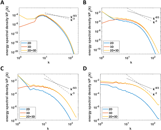
Figure 4. (A–D) Compensated averaged power spectral density of kinetic energy kP2(k) versus horizontal wavenumber k for cases C1 ( ), C3 (
 ), C5 (
 ), and C13 (
 ), respectively. Power spectral densities of 2D, 3D components, and their summation are shown with blue, red, and yellow colors, respectively. Scalings of k−5/3 (Kolmogorov inertial power law) and k−3 (scaling of 2D enstrophy cascade) are shown with solid and dashed lines for reference.
Download figure:
Standard image High-resolution imageTo further illustrate the transfer of kinetic energy among different scales, we define the kinetic energy transfer coefficients from shell Q to shell K (Alexakis et al. 2005; Mininni et al. 2005; Favier et al. 2014) as

where the shells Q and K are defined on the spectral space with horizontal wavenumbers in the range of k ∈ (Q − 1, Q] and k ∈ (K − 1, K], respectively; uQ
and uK
are the corresponding shell filtered velocities; and V is the volume of computational domain. Positive (negative)  means that the kinetic energy is taken from (given to) shell Q and given to (taken from) shell K. The left column of Figure 5 shows
  four selected cases in the four regimes. For the case
  in Regime IV, the flow is not condensed and the kinetic energy is taken from larger scales to smaller scales. However, for the case
  in Regime III, we see from Figure 5 that energy can be directly transferred from small scales (K ≤ 18) to the largest scale. This nonlocal inverse energy cascade provides energy to sustain the formation of the large-scale cyclone. It is in agreement with the results of the previous numerical simulations on RRBC (Favier et al. 2014; Guervilly et al. 2014). For the case
  in Regime II, despite that energy is taken from small scales (5 ≤ K ≤ 22), we also observe a direct energy transfer from the largest scale to moderate scales (K = 4). The reason might be associated with the appearance of an anticyclone. Compared with a cyclone, the convection is more turbulent within the anticyclone because the effective rotating speed is smaller (Käpylä et al. 2011; Chan & Mayr 2013). With more vigorous turbulent motions, the energy is more likely transferred from large scales to small scales. For the case
  in Regime I, the vertical Reynolds number is small and the Ekman number is high, and the rotation effect dominates the buoyant effect at small scales. Thus, we observe that the kinetic energy transfer is cut off at small scales (K ≤ 17). The right column of Figure 5 shows
  , which is the total energy transferred from all Q to a single shell K. A negative value of
  means that the wavenumber K supplies energy, thus this wavenumber can be thought as a forcing wavenumber. From the right column of Figure 5, we see that the forcing wavenumbers for cases C1, C3, C5, and C13, are 7 ≤ K ≤ 11, 2 ≤ K ≤ 13, 2 ≤ K ≤ 12, and 1 ≤ K ≤ 6, respectively. When rotational effect increases, the forcing wavenumbers tend to shift from large-scale wavenumbers to small-scale wavenumbers. In the turbulence regime (Regime IV), the mode K = 1 is a forcing wavenumber. However, it is no longer a forcing wavenumber in other regimes where the rotational effects are dominant.

Figure 5. The left column shows the heatmaps of the kinetic energy transfer coefficients  for shells 1 ≤ Q, K ≤ 60. Positive (negative) value means that energy is taken from (injected to) mode Q. The Rayleigh number is Ra = 108. Note that values close to zero have been removed from the heatmap to signify the major energy transfer processes. The averaged period is about 10 units of time. The right column shows the corresponding values of
  for the left column.
Download figure:
Standard image High-resolution imageTo consider the energy transfer between the 2D and 3D components, we further define the the self- and cross-transfer coefficients as


where  and
and  measure the interactions of the 2D and 3D components of shell Q with the 2D component of shell K, respectively. Figures 6(A) and (C) show the heatmaps of
  and
and  for case C5. From Figure 6(A), we note that the local energy transfer from large to small scales is an important process in self-interaction of 2D components. Apart from the local energy transfer, we also observe a significant direct energy transfer process from moderate scales 3 ≤ Q ≤ 14 to the largest scale K = 1. The cross interaction of 3D and 2D components (Figure 6(C)), however, shows that the moderate scales of 3D component (2 ≤ Q ≤ 6) take energy from the largest scale of 2D component (K = 1). The small scales of 3D component (8 ≤ Q ≤ 48), on the other hand, put energy into the largest scale of 2D component (K = 1). To investigate the net effect of self- and cross -transfer of kinetic energy, we have computed the total energy transfer from all shell Q to a single shell K. Figures 6(B) and 6(D) show
  and
and  as a function of K, respectively. Apparently, the 3D component has a net effect of taking energy from shell K = 1 (Figure 6(D)). However, the 2D component shows a net effect of putting energy into the shell K = 1 (Figure 6(B)), indicating that the LSVs are probably maintained by a 2D self-transfer process in this case.

Figure 6. The left column shows the heatmaps of  and
and  for shells 1 ≤ Q, K ≤ 60 of case C5. Positive (negative) value means that energy is taken from (injected to) mode Q. Note that values close to zero have been removed from the heatmap to signify the major energy transfer processes. The averaged period is about 10 units of time. The right column shows the total energy transferred from the 2D and 3D components of shell Q to the 2D component of shell K, defined as
  and
and  , respectively.
Download figure:
Standard image High-resolution image3.3. Heat Transfer
In this subsection, we discuss the heat transfer in RBBC. To study the 2D and 3D effects on heat transfer, we separate the heat flux into 2D and 3D components. To achieve this, we first split uz
and Θ into two parts, by letting  and
and  . Here,
  and Θ are three-dimensional perturbations from the two-dimensional integrated mean values. Then we can split the convective flux into 2D and 3D components by

where


Here, Fc,2D measures the heat flux transported by 2D convection, and Fc,3D measures the heat flux transported by 3D convection. Both Fc,2D and Fc,3D take average on convective flux temporally and vertically, and thus they are functions of x and y. As mentioned earlier, both cyclonic and anticyclonic regions appear in Regimes II and III. The cyclonic and anticyclonic regions can be shown more clearly after taking temporal and vertical averages. As were shown in the animations for Figures 15 and 16, the cyclonic and anticyclonic regions move around with time, therefore the temporal average cannot be taken for too long a period. For both cases, we take the average for a period of about 20 units of time. The nondimensional system rotation period is 4π Ro, thus the averaged time covers about 18 system rotation periods for case C3 and nine system rotation periods for case C5. Within this time period, the cyclones and anticyclones do not drift too much away.
The results of case C3 (Regime II) and C5 (Regime III) are shown in Figures 7 and 8, respectively. The pattern at Figure 7(E) shows clearly the cyclonic (the region marked by red circle) and anticyclonic (the region marked by blue circle) regions on the contour plot of the averaged vertical component of vortical structure  . Figures 7(A) and (B) show the averaged vertical velocity
  and temperature perturbation
  . Both
  and
and  show structures of twisted rolls in the cyclonic and anticyclonic regions. In simulations of rapidly rotating compressible flow, Chan & Mayr (2013) have found that a cyclone has lower temperature, while an anticyclone has higher temperature in the core region. Our result of RBBC shows different temperature structures in these LSVs. One possible reason may be that our RBBC simulations lack of compressible effect. In Boussinesq flow, the effect of density variation is only considered in the buoyancy term, while the variation on the horizontal direction is ignored. However, in the compressible flow, the horizontal variation of density has significant effect on the horizontal variation of temperature, which may help create a lower (higher) temperature core for a cyclone (anticyclone). Figures 7(C) and (D) show the convective fluxes transported by 2D and 3D components. We note that the 2D component Fc,2D almost transports positive convective flux. The 3D component Fc,3D tends to transport positive convective fluxes in the anticyclonic region. However, in the cyclonic region, the convective flux transported by it can either be positive or negative. It indicates the 3D turbulent motions plays a more important role in transporting convective flux in the anticyclonic region rather than the cyclonic regions. Similar behaviors are observed in Figure 8.

Figure 7. The first five panels in sequence show vertically averaged vertical velocity, temperature perturbation, convective flux transported by 2D barotropic component, convective flux transported by 3D baroclinic component, and vertical component of vorticity. The cyclone and anticyclone (or anticyclonic region) are shown by red and blue circles in the fifth panel (bottom left), respectively. The last panel shows the averaged convective flux in the cyclone (red curves) and anticyclone (or anticyclonic region, blue curves) as functions of radius from their respective center. The average is taken temporally, vertically, and horizontally within the circles plotted in the fifth panel. The case is C3 with Ra = 108 and  . The temporal average period is about 20 units of time.
Download figure:
Standard image High-resolution image
Figure 8. Companion to Figure 7, but for the case C5 with Ra = 108 and  .
.
Download figure:
Standard image High-resolution imageIn order to quantitatively compare the efficiencies of heat transportation between the cyclonic and anticyclonic regions, we take averages on Fc,2D and Fc,3D within the disks around the cyclonic and anticyclonic spots (the centers of the red and blue circles in  ), respectively. Figure 7(F) shows the averaged convective fluxes in the cyclonic and anticyclonic regions for case C3 by red and blue curves, respectively. In the anticyclonic region, the contributions of heat transportation by 2D and 3D components are comparable. However, in the cyclonic region, the heat transportation by the 2D component dominates that by the 3D component. For case C5, the result is different. In the cyclonic region, the heat transportation by 2D and 3D components are comparable. On the other hand, in the anticyclonic region, the heat transportation by the 3D component is much higher than that by the 2D component. By comparing cases C3 and C5, we see that the 2D component plays more and more important role in both cyclonic and anticyclonic regions when rotation rate increases. To verify this trend, we have also computed the averaged convective fluxes transported by 2D and 3D components in case C1. It has been found that the convective flux transported by 2D component is about four times that by the 3D component. From the plot of
  in Figure 9(A), we see that case C1 also contains cyclonic and anticyclonic regions, but we have not found significant difference of convective fluxes transported between these two regions. Although the cyclonic and anticyclonic regions are well separated in an averaged sense (Figure 9(A)), the averaged vertical velocity
  has not shown similar distribution (Figure 9(B)). Apart from
  , both the averaged horizontal velocities
  (Figures 9(C) and (E)) and
  (Figures 9(D) and (F)) have developed shear structures. The shear velocity in the x-direction is larger than that in the y-direction by an order of magnitude. As a result, the group motions of small vortices are more prominent along the x-direction (see animation for Figure 14). If the shear velocities in the x- and y-directions are comparable, then we would expect that LSVs could be formed. To examine whether the shear flow is preferred in the x-direction somehow in the system or just by chance, we continue the simulation of case C1 by switching the x- and y-directions. From the animation for Figure 18, we see that the shear flow is preferred in one direction by chance.

Figure 9. Averaged values for case C1 with Ra = 108 and  . (A–D) Contour plots of the averaged vertical component of vorticity, vertical velocity, horizontal velocities along x- and y-directions, respectively. (E, F) Shear flow velocities as functions of y and x, respectively.
Download figure:
Standard image High-resolution imageFrom the above discussion, we have come to the the following conclusions. First, as rotation rate increases, the 2D effect increases and the 3D effect decreases in transporting convective flux. Second, in Regimes II and III when LSVs appear, heat transfer by convection is more efficient in the anticyclonic region than in the cyclonic region. It is consistent with the observation that convection in the anticyclone is more turbulent because the effective rotation is smaller (Chan & Mayr 2013). In the simulations of Boussinesq flow, Guervilly et al. (2014) also observed a significant reduction of heat transfer inside the cyclone.
3.4. Statistical Results
In this subsection, we investigate the effects of rotation on the statistical results of velocities and Nusselt number. To compare the results among different groups, we use the nonrotating case within each group as a reference case and normalize all the statistical values by the corresponding reference values. Figures 10(A)–(C) show the normalized rms velocities u''/u''∞,  , and
, and  as functions of Ro, respectively. The subscript ∞ denotes the value of the reference nonrotating case. First, we note that the variation of u''/u''∞ on Ro is not monotonic. It shows an increasing trend with increasing Ro in the Regimes I, II, and IV, while a decreasing trend with increasing Ro in Regime III. The trend reversal in Regime III is due to the appearance of large-scale cyclones, in which the flow is dominant by the horizontal large-scale motions. This can be further verified by looking at Figures 10(B) and (C), where the reversal trend is only observed in the horizontal but not in the vertical velocity profiles. Second, we note that the normalized velocities in different groups almost collapse into a single curve in Regime IV. In this regime, the normalized velocities are mainly affected by the convective Rossby number. In the vicinity of Ro ∼ 1 of Regime IV, the normalized vertical velocity is estimated to approximately obey a scaling of
  . In other fast rotating regimes, apart from the convective Rossby number, the normalized velocities also depend on Rayleigh numbers. Cases with higher Rayleigh number tend to have higher normalized vertical velocities. Although the curves of
  for different groups are separated, we still find that
  approximately obeys a scaling of
  in these regimes. Figure 10(D) shows the normalized modified Nusselt number (Nu − 1)/(Nu∞ − 1), where the Nusselt number is defined as
 ![${Nu}=\int \left[{Pe}\langle \overline{{u}_{z}{\rm{\Theta }}}\rangle -\langle \partial \overline{{\rm{\Theta }}}/\partial z\rangle \right]{dz}+1$](https://content.cld.iop.org/journals/0004-637X/923/2/138/revision1/apjac2c68ieqn88.gif) . As seen from the figure, (Nu − 1)/(Nu∞ − 1) always increases with increasing Ro, which indicates that rotation has a negative effect on heat transfer. The slope of (Nu − 1)/(Nu∞ − 1) has a decreasing trend with increasing Ro. In the rapidly rotating regimes (Ro < 0.4), the curves of (Nu − 1)/(Nu∞ − 1) in each group approximately follows a scaling (Nu − 1)/(Nu∞ − 1) ∝ Ro3. It should be mentioned here that the derived scalings of u''z
/u''z
and (Nu − 1)/(Nu∞ − 1) on Ro are empirical results, which currently lack theoretical explanations. In the low Rossby regime, only a few data points are available for the fits. The robustness of these scalings needs to be checked when more data points are available in the future.
. As seen from the figure, (Nu − 1)/(Nu∞ − 1) always increases with increasing Ro, which indicates that rotation has a negative effect on heat transfer. The slope of (Nu − 1)/(Nu∞ − 1) has a decreasing trend with increasing Ro. In the rapidly rotating regimes (Ro < 0.4), the curves of (Nu − 1)/(Nu∞ − 1) in each group approximately follows a scaling (Nu − 1)/(Nu∞ − 1) ∝ Ro3. It should be mentioned here that the derived scalings of u''z
/u''z
and (Nu − 1)/(Nu∞ − 1) on Ro are empirical results, which currently lack theoretical explanations. In the low Rossby regime, only a few data points are available for the fits. The robustness of these scalings needs to be checked when more data points are available in the future.
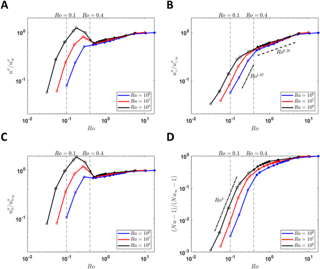
Figure 10. Statistical results of normalized velocities and modified Nusselt number as functions of the convective Rossby number. (A) The total velocity 〈u''〉; (B) The vertical velocity 〈u''z 〉; (C) The horizontal velocity 〈u''h 〉; (D) The modified Nusselt number (Nu − 1). The results are normalized by the reference values of corresponding reference cases. The symbols dot, circle, circle plus, and square represent Regimes I–IV, respectively.
Download figure:
Standard image High-resolution image3.5. Asymmetry between Cyclones and Anticyclones
It has long been found that asymmetry between cyclones and anticyclones emerges in rapidly rotating convection (Chan 2007; Käpylä et al. 2011; Guervilly et al. 2014; Guervilly & Hughes 2017). Guervilly et al. (2014) have discussed several possible mechanisms to explain the asymmetry. The most likely mechanism is that the thermal plumes ejected from the thermal boundary layers tend to induce more cyclonic vorticity. Therefore the clustering of the like-signed cyclonic vorticity favors the formation of the large-scale cyclone. In the low Rossby number limit, both ejection and injection of thermal plumes are allowed in the thermal boundary layer (Vorobieff & Ecke 2002; Sprague et al. 2006). Thus, it is expected that the asymmetry would disappear when Ro is very small (Julien et al. 2012). Guervilly et al. (2014) have studied this mechanism for cases with dominant large-scale cyclone. Here, we extend the discussion of this mechanism across different flow pattern regimes. Following the work of Guervilly et al. (2014), we define the axial vorticity skewness as

the z-dependent axial vorticity skewness as
and the z-invariant axial vorticity skewness as
where dA = dxdy is the differential area element in the horizontal planes.
Figure 11 shows S(z),  , and
, and  for cases C1, C3, C5, and C13. For case C13 (Regime IV), S(z) and
  have a similar structure (Figure 11(C)), with a distribution of large positive values near the thermal boundary layers and small positive values (almost zeros) in the middle of the box. Figure 1 also shows that small but strong cyclonic vortex structures are created in the thermal boundary layers in this case. These vortex structures can only penetrate a short distance, thus the skewness profiles decrease rapidly away from the boundaries. For case C5 (Regime III), a large-scale cyclone appears so that the z-invariant axial vorticity skewness
  has a large positive value (Figure 11(C)). S(z) and
  have a similar profile near the boundaries. In the middle region, S(z) are larger than
  but both of them are positive. From Figure 1, we can see that both cyclonic and anticyclonic vortex structures have been developed in the thermal boundary layers, but the cyclonic vortices are stronger and can penetrate farther away from the boundaries. For case C3 (Regime II), although a pair of cyclone and anticyclone are formed, asymmetry between the cyclone and anticyclone has not completely disappeared (
 is about one in Figure 11(B)). Similar to case C5, both cyclonic and anticyclonic vortex structures have been developed in the thermal boundary layers in case C3 (Figure 1). However, the anticyclonic vortex structures in case C3 are stronger and can penetrate deeper than those in case C5. As a result, the z-dependent axial vorticity skewness
  is close to zero in the middle region (Figure 11(B)). For case C1 (Regime I), anticyclonic structures have similar strengths as cyclonic structures (Figure 1). Since the vortical profile is almost antisymmetric about the middle plane (Figure 1), z-invariant axial vorticity skewness
  is nearly zero (Figure 11(A)). S(z) is positive in both lower and upper half boxes (Figure 11(A)), which indicates that the vortical profile is not exactly antisymmetric (cyclonic vorticity is stronger than anticyclonic vorticity).
  turns to be negative near the boundaries in this case, but its value is too small to draw an affirmative conclusion.
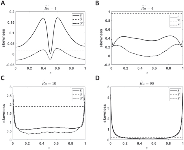
Figure 11. The skewnesses S,  , and
, and  as functions of height. The four panels are for cases C1, C3, C5, and C13, respectively.
Download figure:
Standard image High-resolution imageIn the study of Vorobieff & Ecke (2002), they showed that flow patterns are dominated by cyclonic thermal plumes when Ro ∼ 1. When Ro is further reduced, the number of anticyclonic thermal plumes increases but cyclonic thermal plumes are still favored. Our simulation result agrees well with their experimental studies. Our result also supports the mechanism proposed by Guervilly et al. (2014), that is, the preference for cyclonic thermal plumes might be responsible for the asymmetry between cyclones and anticyclones.
3.6. Comparison with Simulations at Pr = 1
From RBBC simulations at Pr = 1, Favier et al. (2014) reported a higher critical convective Rossby number Roc1 ≈ 0.6 for the appearances of LSVs. In most of their simulations, the aspect ratios of simulation boxes are higher than one (Γ > 1). Guervilly et al. (2014) has also reported that the aspect ratio has impact on the appearances of LSVs. To investigate the effects of Pr and Γ, we have run several simulations at Pr = 1 with different aspect ratios. The simulation parameters are listed in Table 2. First, we notice that from cases D1–D7 that the criteria on the appearance of LSVs at Pr = 0.1 can also be applied to cases at Pr = 1. That is, for Γ = 1, the appearance of LSVs generally requires Ro < 0.4 and  . Figure 12(A) shows the flow structure of case D1. In this case, multiple small vortices appear as the vertical Reynolds number is small. Figure 12(B) shows the flow structure of case D3. Since Ro < 0.4 and
  , a large-scale cyclone appears as expected. Figure 12(C) shows the flow structure of case D7. For this case, Ro = 0.55 and there is no evidence of the appearance of LSVs.

Figure 12. Panels A–E show the horizontal cross sections (at z = 0.2) of the axial vorticity for cases D1, D3, D7, D7b, and D7c, respectively.
Download figure:
Standard image High-resolution imageTable 2. Parameters of Simulation Cases at Pr = 1
| Case | Γ | ℓc | u'' | uz '' | uh '' | Ra | Rez | Ro | E |

| Nu | Regime |
|---|---|---|---|---|---|---|---|---|---|---|---|---|
| D1 | 1 | 0.082 | 0.0606 | 0.0208 | 0.0567 | 3 × 10⁸ | 359.95 | 0.0850 | 4.905 × 10⁻⁶ | 25 | 7.463 | I |
| D2 | 1 | 0.097 | 0.1510 | 0.0430 | 0.1445 | 3 × 10⁸ | 744.42 | 0.1429 | 8.249 × 10⁻⁶ | 50 | 21.259 | III |
| D3 | 1 | 0.116 | 0.2228 | 0.0612 | 0.2140 | 3 × 10⁸ | 1060.08 | 0.2403 | 1.387 × 10⁻⁵ | 100 | 37.563 | III |
| D4 | 1 | 0.128 | 0.2229 | 0.0690 | 0.2116 | 3 × 10⁸ | 1195.18 | 0.3257 | 1.880 × 10⁻⁵ | 150 | 46.023 | III |
| D5 | 1 | 0.138 | 0.1497 | 0.0774 | 0.1272 | 3 × 10⁸ | 1339.81 | 0.4041 | 2.333 × 10⁻⁵ | 200 | 52.596 | IV |
| D6 | 1 | 0.146 | 0.1422 | 0.0819 | 0.1148 | 3 × 10⁸ | 1419.17 | 0.4777 | 2.758 × 10⁻⁵ | 250 | 56.295 | IV |
| D7 | 1 | 0.152 | 0.1369 | 0.0850 | 0.1054 | 3 × 10⁸ | 1472.57 | 0.5477 | 3.162 × 10⁻⁵ | 300 | 59.711 | IV |
| D7b | 2 | 0.152 | 0.1882 | 0.0825 | 0.1685 | 3 × 10⁸ | 1428.41 | 0.5477 | 3.162 × 10⁻⁵ | 300 | 58.275 | III |
| D7c | 3 | 0.152 | 0.2067 | 0.0818 | 0.1893 | 3 × 10⁸ | 1415.96 | 0.5477 | 3.162 × 10⁻⁵ | 300 | 57.983 | III |
| D8 | 1 | 0.048 | 0.0724 | 0.0144 | 0.0709 | 3 × 10⁹ | 786.16 | 0.0548 | 1.000 × 10⁻⁶ | 30 | 9.246 | II |
Note. Γ is the lateral-to-height aspect ratio; ℓc is the critical wavelength for the onset of convection; u'' is the rms velocity; uz
'' is the rms vertical velocity; uh
'' is the rms horizontal velocity; Ra is the Rayleigh number; Rez
is the vertical Reynolds number; Ro is the convective Rossby number; E is the Ekman number;  is the modified Rayleigh number; Nu is the Nusselt number; and the cases are classified into four regimes according to flow patterns. Temporally and spatially (the whole box) averaged values are reported. The grid resolutions are Nx
× Ny
× Nz
= 256 × 256 × 257 for D1–D7, 512 × 512 × 257 for D7b and D8, and 768 × 768 × 257 for D7c.
is the modified Rayleigh number; Nu is the Nusselt number; and the cases are classified into four regimes according to flow patterns. Temporally and spatially (the whole box) averaged values are reported. The grid resolutions are Nx
× Ny
× Nz
= 256 × 256 × 257 for D1–D7, 512 × 512 × 257 for D7b and D8, and 768 × 768 × 257 for D7c.
Download table as: ASCIITypeset image
In the work of Favier et al. (2014), they performed the same simulation as case D7, except that a different aspect ratio with Γ = 3 was used. However, they have observed LSVs in their simulation. Thus, the aspect ratio probably is important to the formation of LSVs (Favier et al. 2014; Guervilly et al. 2014). To investigate the effect of Γ, we performed two companion simulations D7b and D7c with different aspect ratios Γ = 2 and Γ = 3, respectively. Figures 12(D) and (E) show the flow structures of D7b and D7c. Apparently, large-scale cyclones appear in these two cases. This is consistent with the result of Favier et al. (2014). Therefore, aspect ratio indeed affects the appearance of LSVs. Compared to simulations at Γ = 1, the critical convective Rossby number on the appearance of LSVs is higher for simulations at larger Γ.
Favier et al. (2014) have also reported several cases with Ro ≤ 0.1 at Pr = 1 and Γ = 1. In our simulations at Pr = 0.1, we find that a coexisting large-scale cyclone and anticyclone appear when Ro < 0.1 and Rez is large enough. One may ask whether this criterion can be applied to simulations at higher Pr. To investigate this problem, we have run a simulation case at Pr = 1 with Ro = 0.0548 and Ra = 3 × 10⁹. This simulation case was also reported in Favier et al. (2014), but here we have used a higher grid resolution. Figure 12(F) shows that a coexisting large-scale cyclone and anticyclone indeed appear in this case. Thus, the criterion obtained in low Pr regimes is probably also valid in high Pr regimes. An affirmative conclusion requires more simulations across different parameter regimes.
Figure 13 presents a summary of simulation results from different studies. As shown in the figure, for the appearance of LSVs, it requires that Ro is smaller than a certain critical value. We find this critical value is about Ro ∼ 0.4 for a unit box, but Favier et al. (2014) reported a higher value of about Ro ∼ 0.6 for a wider box. The variation of this critical Ro on the size of box needs to be further investigated. A conjecture would be that the critical Ro increases slightly with Γ. The appearance of a coexisting cyclone and anticyclone occurs at a lower critical value Ro ∼ 0.1 in a unit box. Interestingly, Stellmach et al. (2014) found a pair of cyclone and anticyclone at Ro = 0.044 and Pr = 1 in a small box with Γ ≈ 0.22. If the critical Ro indeed increases with Γ, then we would expect that the critical Ro for the appearance of a pair of cyclone and anticyclone is slightly lower than 0.1 in Γ = 0.22. The case in Stellmach et al. (2014) has a Ro = 0.044 < 0.1, which still satisfies the criterion for the emergence of a coexisting cyclone and anticyclone. From the simulation results, we speculate that the criteria for the appearances of LSVs could possibly be universal for flows at different Pr.
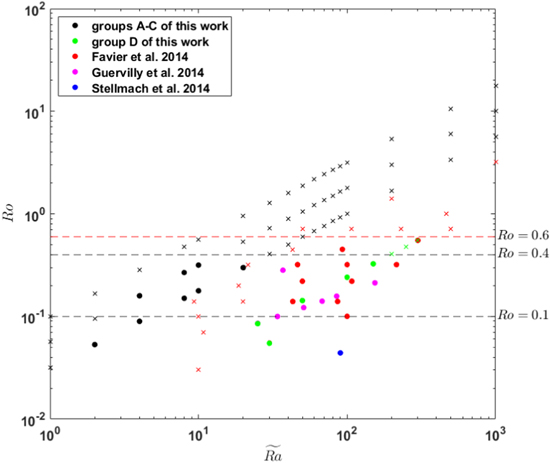
Figure 13. Summary of simulation results from different studies. The black, green, red, magenta, and blue colors represent results obtained from groups A–C of this work, group D of this work, the work of Favier et al. (2014), the work of Guervilly et al. (2014), and the work of Stellmach et al. (2014), respectively. The symbol cross denotes that no LSV appears, and the symbol dot denotes that LSVs appear.
Download figure:
Standard image High-resolution image
4. Summary
In this paper, we present results of numerical simulations on rapidly RRBC at small Prandtl number Pr = 0.1. We have demonstrated that LSVs (both cyclone and anticyclone) can be generated at moderate Rayleigh number with a small Prandtl number. Four different flow regimes are identified in our simulation: the regime of multiple small vortices, the regime of coexisting large-scale cyclone and anticyclone, the regime of the large-scale cyclone, and the regime of turbulence. On the formation of LSVs, two conditions are required to be satisfied: high vertical Reynolds number and low Rossby number. Simulation result suggests that cyclone emerges when the convective Rossby number Ro is smaller than 0.4; the appearance of a coexisting large-scale cyclone and anticyclone requires Ro to be smaller than 0.1. The Reynolds number is also crucial for the formation of LSVs. In the low Rossby range, the flow prefers to form as vertically aligned small vortices instead of LSVs if  . The formation of LSVs requires energy transferred inversely from small scales to large scales. Based on the calculation of the transfer coefficient, we find that the kinetic energy can be directly transferred from small scales to largest scale. The analysis of the 2D flow pattern shows that two separated cyclonic and anticyclonic regions coexist in Regimes II and III. We have investigated the heat transfer efficiency within these two regions. The statistical results indicate that the heat transfer is more efficient in the anticyclonic region. The reason is that the effective rotation rate is smaller in the anticyclonic region than in the cyclonic region. Hence, turbulence is more likely to be freely developed in the anticyclonic region. As a result, the turbulent heat transfer is more efficient in the anticyclonic region. We have also calculated the heat transfer by separating it into the 2D and 3D contributions. The result shows that the 2D contribution increases and 3D contribution decreases in transporting convective flux as rotation rate increases. The effects of rotation on statistical results of normalized velocities and modified Nusselt number (by the corresponding values of reference nonrotating cases) are discussed. We find that the normalized vertical velocity monotonically increases with increasing Ro. It indicates that rotation hinders vertical convection. In the regime of turbulence, the normalized vertical velocity appears to be irrelevant to the Rayleigh number, but mainly dependent on Ro. The normalized vertical velocity tends to follow a 2/7 scaling with Ro in the slowly rotating regime, and a 5/3 scaling with Ro in the rapidly rotating regime. For the heat transfer, we find that the Nusselt number can be drastically reduced with increasing rotation when LSVs or multiple small vortices appear.
Our results may have interesting implications to rapidly rotating gas giants, such as Jupiter and Saturn. In these planets, the Prandtl numbers are estimated to be about 0.1, the convective Rossby numbers of these planets are much smaller than 0.1, and the vertical Reynolds numbers are much higher than 400 (Schubert & Soderlund 2011). Thus, it is anticipated that convectively driven large-scale cyclones and anticyclones can be generated in these rapidly rotating planets. The LSVs observed in these gas giants are probably driven by rapidly rotating convection sustained by the internal heat. It has to be admitted that there is still a gap between the parameters we used in this paper and those of real Jupiter and Saturn. Although a relative simple Boussinesq model is used, the results provide helpful insights on understanding the dynamics of these gas giants. The model we used in this paper can be improved in several aspects. First, here we only consider an incompressible flow, while the atmospheres of these planets are compressible. It seems that compressibility has important effect on the appearance and size of LSVs (Käpylä et al. 2011; Chan & Mayr 2013). The effect of compressibility is worth to be investigated in the future. Second, the Rayleigh numbers we simulated are too low compared to the realistic value of these planets. There is no guarantee that the criteria on the appearance of LSVs obtained in low Rayleigh region can be extended to high Rayleigh regions. It is worthwhile to perform simulations with higher Rayleigh numbers in the future. Third, in this paper, we focus our discussion on an lateral-to height aspect ratio of one. It has been found that the aspect ratio has important effects on the formation on LSVs (Guervilly et al. 2014). Our preliminary study on the effect of aspect ratio indicates that the critical convective Rossby number for the occurrence of LSVs might increase with the aspect ratio. Due to the computational difficulty, most simulations are performed in small or moderate size boxes. In large boxes, multiple LSVs may appear. For example, recent simulations (Cai et al. 2021) in a high aspect ratio (lateral-to-height aspect ratio is 16) box have successfully produced polygonal structures of LSVs. Detailed discussion on the effects of aspect ratio is very expensive. We decide to postpone the exploration to future researches.
I thank the reviewer for helpful suggestions on improving this manuscript. I conceived the idea when I visited the UCLA SpinLab three years ago, and I thank Jonathan Aurnou and the lab members for interesting discussions on rotating Rayleigh–Bénard convection. I appreciate Jing Li and David Jewitt for their hospitality during my visit. I am also grateful to Kwing L. Chan for fruitful discussions on rotating convection in the past years. This work was partially supported by the Guangdong Basic and Applied Basic Research Foundation (No. 2019A1515011625), NSFC (Nos. 12173105, 11503097), Science and Technology Development Fund, Macau SAR (Nos. 0045/2018/AFJ, 0156/2019/A3), the China Space Agency Project (No. D020303), and the China Manned Space Project (No. CMS-CSST-2021-B09). The simulations were performed in the supercomputers at the Purple Mountain Observatory, the National Supercomputer Center in Guangzhou, and the Macau University of Science and Technology.
Appendix A: Supplementary Movies
The animations for Figures 14–17 show the time evolutions of vertical vorticity structures at z = 0.2 for cases C1, C3, C5, and C13, respectively. The time period for each movie is about 37.7 units of time. The animation for Figure 18 shows a companion simulation of case C1 by rotating the domain by 90°.
Figure 14. The animation shows the time evolution of the vertical vorticity structure at z = 0.2 for case C1 (Regime I). The time period for the movie is about 37.7 units of time. The real-time animation duration is 8 s.
(An animation of this figure is available.)
Download figure:
Video Standard image High-resolution image
Figure 15. The animation shows the time evolution of the vertical vorticity structure at z = 0.2 for case C3 (Regime II). The time period for the movie is about 37.7 units of time. The real-time animation duration is 8 s.
(An animation of this figure is available.)
Download figure:
Video Standard image High-resolution image
Figure 16. The animation shows the time evolution of the vertical vorticity structure at z = 0.2 for case C5 (Regime III). The time period for the movie is about 37.7 units of time. The real-time animation duration is 8 s.
(An animation of this figure is available.)
Download figure:
Video Standard image High-resolution image
Figure 17. The animation shows the time evolution of the vertical vorticity structure at z = 0.2 for case C13 (Regime IV). The time period for the movie is about 37.7 units of time. The real-time animation duration is 8 s.
(An animation of this figure is available.)
Download figure:
Video Standard image High-resolution image
Figure 18. A companion simulation of case C1 by rotating the domain by 90°. The time period for the movie is about 37.7 units of time. The real-time animation duration is 8 s.
(An animation of this figure is available.)
Download figure:
Video Standard image High-resolution image