


Abstract
Quasi-periodic pulsations (QPPs) are routinely observed in a range of wavelengths during flares, but in most cases the mechanism responsible is unknown. We present a method to detect and characterize QPPs in time series such as light curves for solar or stellar flares based on forward modeling and Bayesian analysis. We include models for QPPs as oscillations with finite lifetimes and nonmonotonic amplitude modulation, such as wave trains formed by dispersive evolution in structured plasmas. By quantitatively comparing different models using Bayes factors, we characterize the QPPs according to five properties: sinusoidal or nonsinusoidal, finite or indefinite duration, symmetric or asymmetric perturbations, monotonic or nonmonotonic amplitude modulation, and constant or varying period of oscillation. We demonstrate our method and show examples of these five characteristics by analyzing QPPs in white-light stellar flares observed by the Kepler space telescope. Different combinations of properties may be able to identify particular physical mechanisms and so improve our understanding of QPPs and allow their use as seismological diagnostics. We propose that three observational classes of QPPs can be distinguished: decaying harmonic oscillations, finite wave trains, and nonsinusoidal pulsations.
Export citation and abstract BibTeX RIS
1. Introduction
Quasi-periodic pulsations (QPPs) are frequently observed in solar and stellar flares (e.g., Anfinogentov et al. 2013; Pugh et al. 2015, 2017b; Namekata et al. 2017; Hayes et al. 2020). There is no precise definition, but it is generally acknowledged that the amplitude and period modulation are important features (e.g., Nakariakov et al. 2019). Numerous mechanisms have been proposed that can potentially explain QPPs, though it remains an open question which are most common (see, e.g., reviews by Van Doorsselaere et al. 2016; McLaughlin et al. 2018; Kupriyanova et al. 2020). Due to their nonstationary nature, wavelet analysis is commonly used to reveal QPPs in light curves, although care is needed to distinguish oscillations from noise, particularly when there is a strong background trend (e.g., López-Santiago 2018). The temporal and frequency resolution can also be sensitive to the choice of mother wavelet (e.g., De Moortel et al. 2004). The problem of robust identification of QPPs was approached by Broomhall et al. (2019), who tested various methods against synthetic data, demonstrating that forward modeling with Bayesian analysis (e.g., Anfinogentov et al. 2020) and empirical mode decomposition (EMD; e.g., Kolotkov et al. 2015) are the most suitable methods for QPPs with nonstationary periods.
Bayesian analysis is widely used in astronomical data analysis (see review by Sharma 2017), such as the estimation of cosmological parameters (Lewis & Bridle 2002; Wraith et al. 2009) and the search for exoplanets (Nelson et al. 2020). Bayesian analysis is increasingly being applied to data analysis in solar physics (see review by Arregui 2018) such as heliosesmology (e.g., Broomhall et al. 2010; Howe et al. 2015), the inference of longitudinal structuring of coronal loops (Arregui et al. 2013a), and forward modeling of their EUV intensity profiles (Goddard et al. 2017; Pascoe et al. 2017b). In particular, Bayesian analysis has been extensively applied to study transverse oscillations in coronal loops, allowing them to be used as a seismological tool to infer the transverse density structure. These transverse oscillations are simpler than QPPs in having an accepted interpretation in terms of a standing kink mode damped by resonant absorption (e.g., review by Nakariakov & Kolotkov 2020). Kink oscillations were first analyzed by fitting an exponentially damped sinusoid (e.g., Nakariakov et al. 1999), but modern techniques attempt to accurately measure the (nonexponential) amplitude modulation, which contains information about the density profile of the loop (e.g., Hood et al. 2013; Pascoe et al. 2013a, 2019). The nonexponential damping profile may also be revealed through methods such as wavelet analysis (De Moortel et al. 2002) or least-squares fitting (Morton & Mooroogen 2016; Pascoe et al. 2016a, 2016b), but Bayesian methods allow the density profile parameters, which in some cases may only be partially constrained by the data, to be calculated (Arregui et al. 2013b; Pascoe et al. 2017a, 2017d, 2018). Forward modeling of the observed time series also allows detailed properties to be investigated by directly incorporating our physical understanding in the model. For example, Pascoe et al. (2017a) were able to detect the signature of low-amplitude higher longitudinal harmonic kink modes by modeling them as having periods that are approximately integer multiples of the fundamental, having the same start time as the fundamental, and a frequency-dependent damping rate appropriate for resonant absorption. Fourier and wavelet techniques were shown to be unsuitable for the same problem of low-amplitude harmonics (Figure 18 of Pascoe et al. 2017a) since frequency-dependent damping reduces the spectral signature of higher harmonics, whereas forward modeling can correct for this bias. Recently, Pascoe et al. (2020) used Bayesian analysis to distinguish between models of kink oscillations containing either one or two perturbations to test whether loops in an active region had been affected by both solar flares that occurred nearby.
The techniques that have been applied to analyze strongly damped kink oscillations are therefore well suited to study QPPs. In particular, Pascoe et al. (2017d) modeled kink observations that feature rapid shifts in the equilibrium position of the coronal loop in addition to a smoother background trend, including a contracting loop (Simões et al. 2013) whose period of oscillation decreased commensurate with the shortening loop length. In this work we use a similar approach in constructing a model composed of an oscillation, a smooth background, and a rapidly varying background, which in this case represents the sharp increase in flux during the rise phase of a flare.
QPPs have been observed in a range of electromagnetic frequencies, for example, white-light (Mathioudakis et al. 2003; Anfinogentov et al. 2013), microwave (Kupriyanova et al. 2010), EUV (Dominique et al. 2018), X-ray (Mitra-Kraev et al. 2005; Pandey & Srivastava 2009; Hayes et al. 2020), and gamma-ray (Nakariakov et al. 2010; Li et al. 2020), and often in multiple bands simultaneously (e.g., Van Doorsselaere et al. 2011; Dolla et al. 2012; Hayes et al. 2016; Kupriyanova et al. 2019). In this paper we analyze white-light flares observed by the Kepler space telescope (Borucki et al. 2010), though the same method would be applicable to other observations with appropriate models for the behavior of background trends.
Balona et al. (2015) analyzed 257 flares observed by Kepler and found 47 that contained additional peaks and 7 that showed evidence of damped oscillations lasting several cycles. The lack of a correlation for the periods with stellar parameters suggested that the oscillations were due to magnetohydrodynamic (MHD) processes similar to those observed in the Sun. Pugh et al. (2016) analyzed 56 Kepler flares that contained QPPs and found that their properties are independent of global stellar parameters. QPPs have also been detected in stellar flares using the Galaxy Evolution Explorer (GALEX; Doyle et al. 2018), the Transiting Exoplanet Survey Satellite (TESS; Vida et al. 2019), and XMM-Newton (e.g., Broomhall et al. 2019). A comparison of damped oscillations in solar and stellar flares by Cho et al. (2016) demonstrated that the ratios of damping times to periods were statistically identical and that both exhibited a scaling consistent with MHD oscillations.
Bayesian analysis is particularly useful for quantitative model comparison. Since numerous mechanisms for QPPs have been proposed, ideally each mechanism could be tested against observations to identify those most likely. However, detailed theoretical models describing the observable signal for most QPP mechanisms do not currently exist. Therefore, it is currently not possible to test mechanisms directly, but instead we can construct a series of models to investigate particular properties of QPPs with the aim of reducing the possibilities. The properties we focus on are as follows:
- 1.Confirmation of the presence of an oscillation. We examine previously studied examples of stellar QPPs for which confirmation of a QPP is simple. However, since our general model also includes flaring emission, we can test an alternative interpretation of periodically triggered flares (Nakariakov et al. 2006) rather than an oscillation based on a sinusoidal function.
- 2.The oscillation has a finite or indefinite duration, depending on whether it has a well-constrained end time or not.
- 3.Perturbations are either symmetric or asymmetric relative to the background trend.
- 4.Amplitude modulation is monotonic (decreasing) or nonmonotonic.
- 5.Period of oscillation is constant or varying.
Our models for the light curves are described in Section 2, with application to Kepler data in Section 3. Further discussion and conclusions are presented in Section 4.
2. Models
Our method is based on modeling an arbitrary time series, i.e., without detrending and with no particular choice of start and end time for the data. Pugh et al. (2017a) use a method to identify QPPs based on power spectra that does not require detrending but does require that the background trend is not too steep and that the start and end times of the time series are chosen carefully. Inglis et al. (2015) also use a method based on modeling power spectra without detrending and perform a model comparison using the Bayesian information criterion (BIC). The avoidance of detrending is important since the assumption of a particular fixed trend can bias subsequent analysis of an oscillation. This is particularly important for asymmetric oscillations such as strongly damped oscillations or those with higher harmonics present. A longer time series may also better reveal other background trends or noise levels and allows the flare to be studied simultaneously with the QPP, convenient for investigating any dependence of QPP properties on flare properties.
Our general model for a time series consists of three components (though components may be excluded for particular analyses):
- 1.A general background trend that is based on spline interpolation (for three or more interpolation points). The number of interpolation points is chosen to allow an accurate description of the background behavior, depending on factors such as the length of the time series and any long-term trends that are evident (the periodicity associated with the spline background must be longer than that of any QPP).
- 2.An asymmetric function describing a localized increase in flux due to a flare.
- 3.A component based on a sinusoidal function representing an oscillatory QPP.
We model the flaring emission using asymmetric exponential and Gaussian functions with different temporal scales for the rising and decay phases (see examples in Figure 1). We note that the Gaussian profile, previously used in the analysis of synthetic data in Broomhall et al. (2019), was found to provide a poor description of the light curves in this paper, and so we will focus on exponential profiles, though a Gaussian profile may be more suitable for soft X-ray emission (e.g., Gryciuk et al. 2017). The exponential flare profile is
where Af is the amplitude at the peak time tf, τrise is the rise time, and τdecay is the decay time. We impose that the decay time is greater than the rise time, as expected for flares, by considering that τdecay = τriseτratio, where τratio is defined to be greater than 1, typically by using a uniform prior with the limits ![${\tau }_{\mathrm{ratio}}=\left[1,100\right]$](https://content.cld.iop.org/journals/0004-637X/905/1/70/revision1/apjabc69dieqn1.gif) . The rise time can vary significantly for different events, but a range of
. The rise time can vary significantly for different events, but a range of ![${\tau }_{\mathrm{rise}}=\left[0.1,50\right]$](https://content.cld.iop.org/journals/0004-637X/905/1/70/revision1/apjabc69dieqn2.gif) minutes was found to be suitable for those in this paper. Flare amplitude can also vary significantly, but our normalization of the time series ensures that a range of
minutes was found to be suitable for those in this paper. Flare amplitude can also vary significantly, but our normalization of the time series ensures that a range of ![${A}_{f}=\left[0,1.5\right]$](https://content.cld.iop.org/journals/0004-637X/905/1/70/revision1/apjabc69dieqn3.gif) is sufficient. Here, values above 1 are permitted for estimation of uncertainties when Af ≈ 1. (Similarly, in some cases the background trend may be very close to 0, and so a suitable prior for background parameters is [−0.1, 1].) For models with a single flare the prior
is sufficient. Here, values above 1 are permitted for estimation of uncertainties when Af ≈ 1. (Similarly, in some cases the background trend may be very close to 0, and so a suitable prior for background parameters is [−0.1, 1].) For models with a single flare the prior ![${t}_{f}=\left[\min \left(t\right),\max \left(t\right)\right]$](https://content.cld.iop.org/journals/0004-637X/905/1/70/revision1/apjabc69dieqn4.gif) may be used, but for cases with multiple flares more specific estimates preserve the order of the flares and so avoid degeneracy.
may be used, but for cases with multiple flares more specific estimates preserve the order of the flares and so avoid degeneracy.
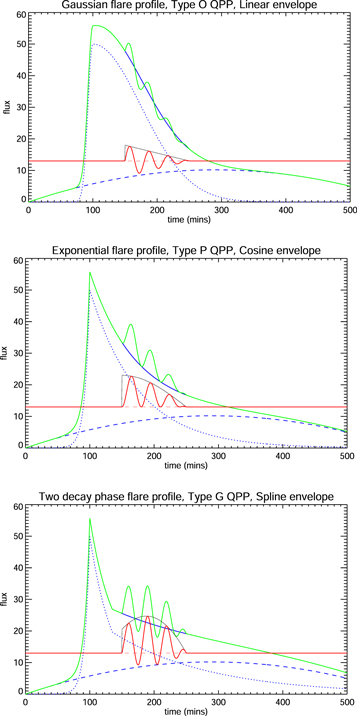
Figure 1. Examples of light-curve models featuring a flare and QPP. The light curve (green line) is composed of a background (solid blue line) and a QPP modeled as an oscillation with a finite duration. The QPP component is shown separately as a solid red line, with the dashed red line representing zero perturbation (shifted for visibility). The thin black line represents the envelope of the QPP. The background consists of a flare (dotted blue line) and a spline component (dashed blue line). Type O, Type P, and Type G QPPs are distinguished based on how they contribute to the total flux, as described by Equations (3)–(5), respectively.
Download figure:
Standard image High-resolution imageDavenport et al. (2014) studied the temporal morphology of thousands of white-light flares on the M dwarf star GJ 1243 (KIC 9726699) and found that the decay phase is best described using two exponential regimes. These two decay profiles describe impulsive and gradual cooling phases associated with blackbody and red continuum emission, respectively (Kowalski et al. 2013). In our models the spline component is capable of describing slower variations in the background, but we can also explicitly include a second decay phase in our model as required, with the form
where the amplitude  at the start of the second decay phase t2, after which the decay time is τ2, which is defined to be greater than τrise, as with τdecay.
We consider two main forms for the sinusoidal function describing the QPP, as well as a generalized model that can reduce to either case. The first (Type O; oscillatory) is the common form

with amplitude A, period of oscillation P, frequency ω = 2π/P, and start time t0, with  . The second form (Type P; positive) is

which defines the oscillatory perturbations to be strictly positive. The second form is related to the square of the first form via the identity  , but the version given in Equation (4) retains the same definition of the amplitude and period of oscillation as Equation (3). This is convenient for parameter estimation since the same values may be used for both models. We note that we model the periodicity associated with the observed signal, which is not necessarily the periodicity of the underlying physical mechanism since it also depends on how the observed emission is generated.
We can also consider a general (Type G) form for the oscillation

with a phase shift ![$\phi =\left[0,\pi /2\right]$](https://content.cld.iop.org/journals/0004-637X/905/1/70/revision1/apjabc69dieqn8.gif) , where lower and upper limits correspond to Type O and Type P oscillations, respectively. Alternatively, we can characterize the asymmetry of the QPP in terms of the positive fraction
, where lower and upper limits correspond to Type O and Type P oscillations, respectively. Alternatively, we can characterize the asymmetry of the QPP in terms of the positive fraction

with limits of 0.5 (Type O) and 1 (Type P). A comparison of models for Types O, P, and G allows us to test for and potentially quantify any asymmetry in the oscillation. The asymmetry of the oscillation may be related to the mechanism that generates the observational signal. For a particular mechanism this could be modeled directly. We note, however, that these functions do not describe any distortion to the sinusoidal profile, which might also arise for a nonlinear relationship between the physical perturbation and the observed emission.
For the oscillations described above the start time t0 is a time for which the sinusoidal function is zero. The localization of the QPP in time is described by the chosen form of the amplitude modulation. A common choice is a decay profile of the form  with a decay time τ and exponent n. Exponential and Gaussian decay profiles are given by n = 1 and 2, respectively. An exponential profile or half-Gaussian profile, each nonzero for
  , describes monotonic amplitude modulation but without a defined end time. As in Pugh et al. (2016), we can also consider a full Gaussian profile to describe nonmonotonic amplitude modulation, in which case there is also no defined start time and t0 corresponds to the time of maximum amplitude.
However, our main focus is on models that describe QPPs as having an explicit end time rather than, or in addition to, harmonic oscillations defined on an infinite or semi-infinite interval. The detection of a well-defined end time can assist in the identification of the QPP mechanism or interpretation of the signal duration. For example, in the case of quasi-periodic wave trains generated by an impulsive perturbation of an inhomogeneous plasma, the duration of the wave train is determined by dispersion (e.g., Roberts et al. 1983), with a characteristic "tadpole" signature generated by perturbations that are sufficiently localized in space and time (e.g., Nakariakov et al. 2004, 2005; Goddard et al. 2019).
We consider several oscillation envelopes that have explicit start and end times. The amplitude of each of the envelopes is defined as 1 at the start time t0 and 0 at the end time t1. A finite lifetime for the QPP also has the practical benefit of providing a finite time for which any period modulation also needs to be considered. In contrast, for an exponential damping profile the QPP would continue to exist indefinitely with a vanishingly small amplitude unconstrained by the data (which is often quite noisy), and so any period modulation would also be unconstrained. This is a key issue since accurate detection of amplitude and period modulation in QPPs is essential to identifying the mechanism responsible.
Oscillation envelopes considered in this work are a linear decrease

a cosine function (quarter of a cycle from 1 to 0)

and a spline envelope

The spline envelope starts at 1 and ends at 0, with one or more points  in between that are free parameters of the model. The linear and cosine envelopes are monotonically decreasing by definition, whereas for the spline envelope the priors for the interpolation points yi can include values greater than 1, which allows this envelope to describe nonmonotonic amplitude modulation. Examples of these three envelopes are shown in Figure 1. The linear, cosine, and spline envelopes shown are qualitatively similar to exponential, half-Gaussian, and full Gaussian decay profiles, respectively, but having explicit start and end times rather than being defined on a semi-infinite or infinite interval.
3. Results
We demonstrate our method by applying it to several QPPs observed during white-light stellar flares by the Kepler space telescope and compare our results to previous analysis. The observational data are the simple aperture photometry (SAP) light curves. The statistical study by Pugh et al. (2016) demonstrates that the QPP properties are not correlated with the emission amplitude, so for convenience we normalize each of our light curves to the range [0, 1]. The dates and normalization fluxes for our observational data are noted in Table 2. We compare our models to the observational data using a version of the Solar Bayesian Analysis Toolkit (SoBAT; Pascoe et al. 2017a; Anfinogentov et al. 2020) for Markov Chain Monte Carlo (MCMC) sampling. Our calculations are based on 2 × 10⁶ MCMC samples for each model, with a burn-in stage of 105 samples, which is found to be sufficient for the problems in this paper. The burn-in stage ensures that our parameter results are independent from their initial estimates and that the main sampling begins in a region of the parameter space with high probabilities. Model parameters use uniform prior probability density functions, except where stated that results from previous analysis by Pugh et al. (2016) are used to define a normal prior. By definition FP must be in the interval [0.5, 1], but for other model parameters estimates are used to define the limits, which are checked using the posterior probability density function to ensure that they are not unreasonably restricting the parameter values. Prior limits are also used to avoid unnecessary degeneracy in models, for example, in a model with multiple flares their times are restricted so as to preserve the order in which they occur.
SoBAT generates samples using the Metropolis–Hastings algorithm (Metropolis et al. 1953; Hastings 1970) with the multivariate normal distribution used as the proposal distribution. The covariance matrix is automatically tuned to keep the acceptance rate in the range of 10%–50% during sampling, to ensure efficient sampling of the high-dimensional parameter space. If the acceptance rate becomes too high or too low, the step size is retuned and the chain is restarted. We assume that the error in our data is normally distributed with a standard deviation of σn, which is considered as an additional free parameter in our models. In this paper we consider models with 6–27 free parameters, which the SOBAT code is well suited to consider. For problems with a far greater number of free parameters alternative MCMC strategies can be used (e.g., Haario et al. 2004).
3.1. KIC 2852961
In their analysis of this QPP, Pugh et al. (2016) calculate an adjusted flux by subtracting a smoothed version of the time series. This method can generate spurious results when applied to a rapidly changing signal, such as the rising phase of a flare. This problem is avoided in Pugh et al. (2016) by only considering the decaying phase of the signal and cropping the time series accordingly. Here we first consider a similarly cropped time series but model the background simultaneously with the QPP rather than detrending. In this case, the general background component (a spline with five interpolation points) is found to be sufficient to describe the slight rise and subsequent decay of the flux, so here we do not include a flare component such as Equation (1), which includes a large, rapid rise phase.
Pugh et al. (2016) take the time of maximum flux to be the start time for their adjusted flux (with times before this considered to be negative). However, it is evident in the top left panel of their Figure B1 that the QPP likely starts before this time, in which case their first zero of the sinusoidal oscillation might actually be closer to a maximum. (This also means that their QPP oscillation has an initially negative perturbation.) Their fitting method estimates the period of the QPP as P = 67 ± 1 minutes and a decay time of τ = 27 ± 2 minutes, with a Gaussian decay profile found to be better than an exponential one. In general, the Gaussian profile of Pugh et al. (2016) includes the increasing phase as well as the decreasing phase, with the time of maximum amplitude determined by their parameter B = 35 ± 2 minutes−2. In Figure B1 of Pugh et al. (2016) the fitted damping profile appears to significantly underestimate the maximum at ≈100 minutes, suggesting that a Gaussian profile eventually becomes too strong, though the behavior for the first few extrema justifies its choice over an exponential decay profile.
Results of our analysis are shown in Figure 2. Here our time series starts and ends at approximately the same times as shown in Figure B1 of Pugh et al. (2016). However, each of our models is applied to the full time series shown, whereas in Pugh et al. (2016) only the time after peak flux (here ≈55 minutes) was considered. In the top panels we first consider a model with no QPP component, i.e., just a spline background using five interpolation points. The total number of parameters in this model is therefore np = 6 including the observational noise σn.

Figure 2. Model for the decay phase of KIC 2852961 without a QPP (top panels) and for our strongest QPP model (bottom panels). The middle panels correspond to a Gaussian decay profile similar to that considered by Pugh et al. (2016). The left panels show the model fit based on the maximum a posteriori probability (MAP) parameters, with line styles as described in Figure 1 (as for other figures). np is the number of free parameters in the applied model. The right panels show the posterior predictive distribution (PPD), with contours corresponding to 1σ, 2σ, and 3σ confidence levels. σn is the estimated level of noise in the data when described by the corresponding model.
Download figure:
Standard image High-resolution imageThe significance of an oscillatory QPP in a time series can be quantified by comparing the Bayesian evidence for the model that includes the oscillation to a model without the oscillation but otherwise the same. However, this relies on the Bayesian analysis for the model with a QPP having already been done. We can consider the problem of identifying the need for a QPP from a model containing only the background components. From the posterior predictive distribution (PPD) for our model without a QPP (top right panel of Figure 2) it can be seen that the data points that exceed the 1σ confidence level do so in a manner that is consecutive, oscillatory, and mainly during the first part of the signal. This is consistent with there being a localized oscillatory feature missing from the model. The PPD histograms in this paper are based on normally distributed noise, with the level of the noise σn being an additional free parameter of the model. We expect for a reasonable model that approximately 68% of the data points should fall within the 1σ region, and those that lie outside it should be distributed throughout the time series in an unbiased manner. The lack of a QPP in the model means that the level of the noise is overestimated to attempt to account for the systematic error from the oscillatory behavior. We can perform quantitative tests to check our assumption that the model residuals χ are normally distributed. Figure 3 shows the one-sample Kolmogorov–Smirnov tests for the models shown in Figure 2. This test is based on the maximum absolute distance (located by the dotted line and highlighted in red) between the cumulative distribution function (CDF) for the proposed distribution (here a normal distribution) and the empirical cumulative distribution function (ECDF) for the model residuals based on the maximum a posteriori probability (MAP) values for model parameters. We also calculate the one-sample Anderson–Darling test, which considers the difference over the entire CDF rather than just the maximum difference. Our Kolmogorov–Smirnov and Anderson–Darling tests use μ = 0 and σn as estimated from our MCMC sampling to calculate the CDF. We also apply the Lilliefors test for normality, which uses a mean and standard deviation calculated from the residuals themselves. This tests whether the residuals are described by some normal distribution even if not the specific distribution  that our MCMC sampling estimates. Using critical values based on a significance value of α = 0.05, we find that the model without a QPP fails all three of these normality tests, whereas the models with a QPP pass all three. We note that model residuals might also fail normality tests in the case of a different noise distribution, such as a Poisson distribution for very low flux measurements, though this is not the case for the observations in this paper.

Figure 3. One-sample Kolmogorov–Smirnov tests for the models shown in Figure 2. For a significance value of α = 0.05 the model with no QPP (top) fails the test for normality, while the models with QPPs with Gaussian (middle) and spline (bottom) envelopes both pass.
Download figure:
Standard image High-resolution imageThe above tests are therefore useful in identifying a weak model that can be improved, but we will focus on the use of Bayes factors to quantitatively compare detailed models for the purpose of characterizing the QPPs. A strength of the Bayes factor is that it considers the model behavior over the entire parameter space rather than tests that only make use of a single point (e.g., the MAP values) such as the three mentioned above and others such as BIC. Furthermore, Bayes factors are suitable for comparison of non-nested models, for example, our comparison of different QPP envelopes, and Type O versus Type P QPP models.
We applied different QPP models for the different properties described in Section 2. The middle panels of Figure 2 show results for a Type O QPP with a Gaussian decay profile, similar to that used by Pugh et al. (2016), except here the analyzed time series extends earlier than the time of peak flux (≈55 minutes). As in the previous analysis, we find that the imposition of the Gaussian profile underestimates the peak at ≈160 minutes owing to the constraint that the oscillation appears to end shortly after this time, which requires a short decay time.
The bottom panels of Figure 2 show the results for our model that best describes the time series (based on Bayes factors discussed below), which is a Type G QPP (FP ≈ 0.8) with spline envelope and constant period of oscillation. This model has explicit start and end times, and so the localization of the QPP in time does not depend on the shape of the amplitude modulation alone, as is the case for the Gaussian decay profile, for which the localization is implied through the decay time. This allows us to characterize the amplitude modulation independently of the localization in time by considering different envelopes, such as the additional examples shown in Figure 4 and summarized in Table 1.

Figure 4. Models for KIC 2852961 with Type O (left) and Type P (right) QPPs, with linear (top), cosine (middle), and spline (bottom) envelopes.
Download figure:
Standard image High-resolution imageTable 1. Models for KIC 2852961 (Cropped Time Series)
| Type | Envelope | t0 (minutes) | t1 (minutes) | P0 (minutes) | P1 (minutes) | A0 | A1 | FP | KQ0 |
|---|---|---|---|---|---|---|---|---|---|
| O | Linear |

|

|

|
⋯ |

|
⋯ | 0.5 | 361 |
| Cosine |

|

|

|
⋯ |

|
⋯ | 0.5 | 390 | |
| Spline |

|

|

|
⋯ |

|

|
0.5 | 418 | |
| Spline |

|

|

|

|

|

|
0.5 | 414 | |
| P | Linear |

|

|

|
⋯ |

|
⋯ | 1 | 255 |
| Cosine |

|

|

|
⋯ |

|
⋯ | 1 | 310 | |
| Spline |

|

|

|
⋯ |

|

|
1 | 442 | |
| Spline |

|

|

|

|

|

|
1 | 442 | |
| G | Linear |

|

|

|
⋯ |

|
⋯ |

|
355 |
| Cosine |

|

|

|
⋯ |

|
⋯ |

|
385 | |
| Spline |

|

|

|
⋯ |

|

|

|
449 | |
| Spline |

|

|

|

|

|

|

|
447 | |
Note. Posterior summaries correspond to the MAP value and 95% confidence interval. P0 is the constant or initial period of oscillation. P1 is the final period of oscillation for models with a linear variation. A0 is the initial amplitude of the envelope. A1 is the additional free parameter for the spline envelope, corresponding to the amplitude at the center of the envelope relative to the initial amplitude. FP is the positive fraction given by Equation (6). KQ0 is the Bayes factor for each model compared with the model without a QPP.
Download table as: ASCIITypeset image
The Gaussian and spline models discussed above each provide a good description of the oscillatory behavior in the light curve, and the results are qualitatively similar. Both models pass all three normality tests for residuals, whereas the model without a QPP failed all three. The sums of the absolute values of the residuals are also nearly identical, so these tests based on the MAP parameters do not allow us to differentiate the models. The Bayes factor (Jeffreys 1961) provides more robust model comparison by taking the entire parameter space into account. The Bayes factor comparing model i with model j is

where Bij is the ratio of Bayesian evidence for model i to model j. The Bayes factor for the spline envelope model compared with the Gaussian decay model is KSG = 19. The value being greater than 10 indicates very strong evidence (e.g., Kass & Raftery 1995) in favor of the model with a spline envelope. We can consider this as a measure of our confidence in the QPP having a finite duration since it compares our strongest model with explicit start and end times to our strongest model without these. On the other hand, the Gaussian decay model outperforms models with cosine (KGC > 40) and linear (KGL > 69) envelopes, indicating that the nonmonotonic amplitude modulation is a much stronger feature of the QPP than the finite duration.
In Table 1, the Bayes factor KQ0 compares each model to that with no QPP (top panels of Figure 2), and as expected, all of them greatly exceed the threshold for very strong evidence. The Bayesian evidence favors Type O QPPs over Type P for both the linear and cosine envelopes but favors Type P when using the spline envelope. The Bayes factor for the Type P spline compared to the Type O spline is KPO = 24, indicating very strong evidence. These results demonstrate the importance of accurately modeling the amplitude modulation since the evidence for a Type P QPP only becomes apparent when allowing the nonmonotonic amplitude modulation. This is due to the large amplitude of the second peak, which cannot be accounted for by either the linear or cosine envelopes, which are monotonically decreasing. However, for Type O models there is flexibility to adapt to this by shifting the location of the equilibrium, whereas for Type P models the equilibrium is effectively constrained to follow the local minima of the flux since the perturbations are defined to be positive only. When the spline envelope is used and the amplitude modulation is permitted to be nonmonotonic, the constraint on the background trend no longer disadvantages the Type P QPP model, and it provides the best description of the light curve. This behavior is also seen in the results for the Type G models, with the positive fraction being FP ≈ 0.5 for linear and cosine envelopes, but being well constrained with FP ≈ 0.8 for a spline envelope.
We also see how the asymmetry of the QPP affects the estimate for the start time, with Type P models having an earlier start time in accordance with the longer time required to reach the first maximum. This difference is approximately a quarter of the period of oscillation. The period of oscillation is approximately 56 minutes compared to 67 ± 1 found by Pugh et al. (2016), though this difference can be accounted for by the different interpretation of the start time of the QPP. The associated uncertainty is slightly smaller in our method with σP ≈ 0.5 minutes.
We examine whether the QPP has a varying period of oscillation by considering models with a linear variation from P0 to P1 at the start (t0) and end (t1) times, respectively, i.e.,

The results in Table 1 show that for models with a varying period the credible intervals significantly increase compared to those for a constant period, indicating poor constraint of the parameters by the data. The Bayes factor for the equivalent nonstationary model compared to the strongest stationary model is KNS = 1.9. The value is positive, i.e., in favor of a varying period, but the magnitude is less than 2, which is the minimum threshold to be considered "positive" rather than "not worth more than a bare mention" (Kass & Raftery 1995).
To summarize (see Table 2), we find that the evidence for the QPP is conclusive and the strongest model is a Type G oscillation with finite duration, nonmonotonic amplitude modulation, and a constant period of oscillation.
Table 2. Summary of Our Observations and Results
| Date (BKJD) | Flux (e− s−1) | Modulation | |||||||
|---|---|---|---|---|---|---|---|---|---|
| KIC | Start | End | Minimum | Maximum | Sinusoidal | Duration | Type | Amplitude | Period |
| 2852961 | 405.18 | 405.43 | 1283030 | 1288860 | Yes | Finite | G | Nonmonotonic | Constant |
| 404.95 | 406.20 | 1279290 | 1288860 | Yes | Finite | P | Nonmonotonic | Decreasing | |
| 12156549 | 454.7 | 455.3 | 6048.44 | 6871.48 | No | (Finite) | (P) | (Nonmonotonic) | (Constant) |
| 9726699 | 568.145 | 568.252 | 266668 | 272530 | Yes | Indefinite | O | Exponential | Constant |
| 6184894 | 1410.7 | 1411.3 | 70288.4 | 71407.2 | Yes | Finite | P | Nonmonotonic | Constant |
Note. Dates correspond to the Kepler Barycentric Julian Day (BKJD). We characterize the QPPs according to five properties. For KIC 2852961 we consider two time series lengths for the same event. For KIC 12156549 the strongest model is nonsinusoidal, but for comparison we include the characteristics of our strongest sinusoidal model in parentheses.
Download table as: ASCIITypeset image
Our conclusion of a constant period of oscillation applies to the time series used in this section, which is cropped around the decay phase of the flare as in Pugh et al. (2016). Next, we consider an extended time series for the same event and find evidence for a decreasing period. However, we stress that this is not due to our method itself being sensitive to the choice of start and end times (as can be the case with Fourier/wavelet analysis). Instead, extending the time series presents an additional local maximum (at ≈300 minutes in Figure 5), which we model as also being part of the QPP. This additional oscillation cycle has a longer periodicity than the subsequent ones, and so the QPP model better describes the data when using a varying period of oscillation.

Figure 5. Analysis of KIC 2852961 using an extended time series featuring multiple flares. The top left panel shows the PPD for a model without a QPP. The right panels show the MAP components of models with Type O (top) and Type P (bottom) QPPs. The bottom left panel shows wavelet analysis for the detrended light curve. The green line shows the signal after detrending with the background from the Type P QPP model (shifted for visibility). The color contour represents the normalized wavelet power, and the hatched region is the cone of influence. The dashed line shows the modeled period variation (MAP values).
Download figure:
Standard image High-resolution imageFigure 5 shows the same event with the time series extended on both sides of the QPP to include the rise phase of the flaring emission. This demonstrates the inclusion of the flare component(s) of our model. There appear to be three flares during the extended time series that we model with exponential rise and decay phases. We assume that the rise and decay times are the same for each flare. To avoid degeneracy, the priors for the times of the flares are defined by the nonoverlapping intervals [125, 140], [275, 300], and [755, 780] minutes. There appear to be significant deviations from an exponential decay, seen most clearly during the decay phase of the third flare (∼1000 minutes). This behavior does not resemble two exponential decay phases either, and it appears to be approximately linear. Our spline background component (dashed blue line) is able to describe this behavior without the need to modify the form of the flare component.
The right panels of Figure 5 show the results for Type O (top) and Type P (bottom) QPP models. For this extended time series, the very strong evidence for an asymmetric QPP remains (KPO = 809), although Type G is no longer stronger than Type P (KPG = 5.7). The evidence for a (linearly) varying period of oscillation, described by Equation (11), is very strong (KNS = 96) for this extended time series, which includes the additional cycle at ≈300 minutes. The period of oscillation decreases by 19% over the lifetime of the QPP, and the shape of the QPP resembles an impulsively generated quasi-periodic wave train formed by the dispersive evolution of MHD waves. This is also seen in the bottom left panel of Figure 5, which shows the wavelet analysis (using the code by Torrence & Compo 1998) of the detrended light curve with the characteristic tadpole signature (Nakariakov et al. 2004).
3.2. KIC 12156549
Figure 6 shows our time series for this event, which is again extended in comparison to Figure 1 of Pugh et al. (2016) to show more of the background behavior. This highlights a smaller flare just before the main one and a long-term background that appears to be flat (which we model as being constant rather than using a spline background component). There are four strong peaks in the light curve. Unlike the previous example, the difference between peaks that should be attributed to flares and those that are part of an oscillation is not so clear. This suggests two alternative models: two flares with an oscillatory QPP, or four flares without an oscillatory QPP. The latter case could still be considered a QPP, as the repetitive triggering of flares is also a proposed mechanism for generating QPPs in emission. Quantitatively comparing these two interpretations is a non-nested model comparison problem, which Bayesian analysis is well suited to.
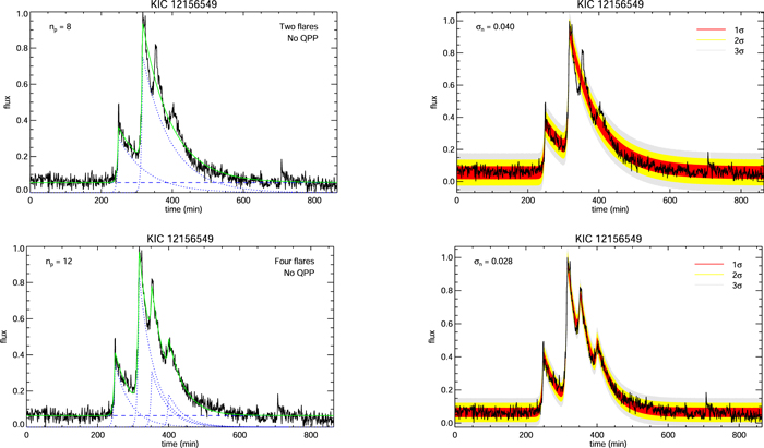
Figure 6. Models for KIC 12156549 with a constant background and no QPP component: two flares (top) and four flares (bottom), each of which is modeled using the asymmetric exponential profile in Equation (1).
Download figure:
Standard image High-resolution imageResults of models without an oscillatory component are shown in Figure 6. As in the previous example, for multiple flares we assume that the rise and decay times are the same for each flare. For the model with four flares, the priors for the flare times are defined by the intervals [245, 260], [310, 325], [345, 360], and [395, 420] minutes (models with two flares use the first two of these). The model with two flares is clearly insufficient, and the residuals fail our three tests for normality (see Figure 7). However, the model with four flares provides a very good description of the light curve, and its residuals pass the three normality tests. The Bayes factor for four flares compared with two is K42 = 562.
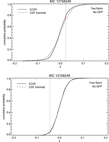
Figure 7. One-sample Kolmogorov–Smirnov tests for the models shown in Figure 6. For a significance value of α = 0.05 the model with two flares (top) fails the test for normality, while the model with four flares (bottom) passes.
Download figure:
Standard image High-resolution imagePrevious analysis of this event is shown in Figure 1 of Pugh et al. (2016) and was found to have a period of 44.6 ± 0.6 minutes and Gaussian profile with decay time 36 ± 2 minutes and B = 28 ± 2 minutes−2. In the previous example (Section 3.1) we had a different interpretation of the start time of the oscillation and so obtained a different period of oscillation. That is not the case here, and so we can make use of the previously reported mean period and its standard deviation to define a normal prior for the period in our analysis. Based on the Gaussian decay profile with B > 0, we can also expect a spline envelope to provide the best description. Results of models with two flares and an oscillatory component are shown in Figure 8. For the oscillatory QPP models, we find that Type P is better than Type O (KPO = 60), and Type G provides no further improvement (KPG = 0.1). There is also strong evidence against a varying period of oscillation (KNS = −6.1) based on comparing a model with a linearly varying period to one with a constant period. However, the four flare model remains remarkably better than the Type P model (K4P = 112).
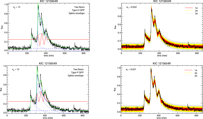
Figure 8. Models for KIC 12156549 with two flares and a QPP with spline envelope: Type O (top) and Type P (bottom).
Download figure:
Standard image High-resolution imageThese results demonstrate very strong evidence for a multiflare model over an oscillation model for this QPP (or at least over the simple sinusoidal oscillations considered in this paper). The apparent periodic nature of the three later flares may simply be coincidental. However, we can also consider the mechanism of the quasi-periodic modulation of flaring emission by an MHD oscillation (Nakariakov et al. 2006). We can speculate that the first flare generated an oscillation in a loop or structure, which then triggered periodic flaring energy release in an associated active region. This is consistent with the amplitude and timing of the first flare appearing to be different from the three subsequent ones. The decrease in flare amplitude in time may also be interpreted as each subsequent flare having less energy stored in the flaring system to release. Oscillatory reconnection can also generate periodic outputs, without the need for an oscillating structure. An impulsive phase is followed by a stationary phase resembling a damped harmonic oscillator (McLaughlin et al. 2012). Alternatively, the signal might be better described by a nonlinear or multiharmonic oscillation with cycles that are more triangular than the sinusoidal function used in this paper. In both our analysis and a previous one by Pugh et al. (2016), the main limitation of sinusoidal models appears to be the significant underestimation of the local maximum at ≈350 minutes.
3.3. KIC 9726699
Here we consider an example for which the strongest QPP model is that of an exponentially damped sinusoid. This was selected from the examples in Pugh et al. (2016) on the basis of their analysis supporting an exponential decay profile with a large decay time, and we again use their estimates (P = 24.2 ± 0.1 and τ = 133 ± 33) to define our Bayesian priors.
The statistical study by Davenport et al. (2014) found over 6100 flares in KIC 9726699 and, after suitable rescaling in amplitude and duration, was able to fit detailed models to the rise and decay phases. The rise phase was fit by a fourth-order polynomial. The decay phase was fit using two separate exponential profiles, and with an improved model that smoothed out the transition between phases. For this flare the rise time is short, and so we continue to use an exponential rise phase, rather than a polynomial, but we include the two exponential decay phases found by Davenport et al. (2014), as described in Equation (2). We also have a smooth background component that helps improve our total background trend.
The analysis for our strongest model is shown in the top panels of Figure 9. The background uses a spline component based on five interpolation points and a flare with two decay phases (we find very strong evidence against a single decay phase K = −73). For this time series we choose to place one interpolation point just before the flare (at t = 15 minutes). This allows the model to better describe the short preflare signal than equally separated interpolation points would allow (and without increasing the number of points such that one would be there when equally separated). This model differs from Pugh et al. (2016) (see their Figure B7), in which the QPP begins at the time of maximum flux. We can consider an equivalent model using our method, shown in the bottom panels of Figure 9, though we find very strong evidence against it (K = −32).

Figure 9. Models for KIC 9726699 with a flare with two decay phases and an exponentially damped QPP. The top panels represent our strongest model, while the bottom panels correspond to a model for which the QPP start coincides with a peak flux similar to that considered by Pugh et al. (2016).
Download figure:
Standard image High-resolution imageAside from this different start time, our results are consistent with those of Pugh et al. (2016); we find an exponential decay profile to be better than a Gaussian (KGE = −2.7), and no evidence of asymmetry (KPO = −1.2). The evidence for the oscillation is very strong (KQ0 = 38), but there is no evidence for a nonstationary period of oscillation (KNS = 0.1). (For an exponential damping profile with a varying period, t1 in Equation (11) is taken to be the end of the time series.) There is strong evidence against a finite oscillation with a spline envelope (K = −6.0), consistent with the oscillation retaining a measurable amplitude until the end of the time series and so not having a well-defined end time. We cut our time series just before a discontinuity in the data that may be an instrumental effect, but even still the signal quality (τ/P ≈ 4.7) is significantly higher than that observed in our examples of finite wave trains.
3.3.1. Interpretation as Standing Hydrodynamic Mode
In this paper our aim is to characterize QPPs by testing different functional forms for the oscillatory behavior. However, it is also desirable to consider specific mechanisms where possible, as has been demonstrated in the Bayesian analysis of kink oscillations in coronal loops. A large number of mechanisms have been proposed, but currently there are few testable predictions that can be used to distinguish them observationally. For this event our method supports the interpretation in terms of an exponentially damped sinusoid. This oscillatory behavior is commonly associated with standing modes in waveguides such as coronal loops. Since the oscillation has a long period and modulates the plasma emission, a possible interpretation is a standing slow MHD mode. Another possibility is a standing hydrodynamic mode proposed by Reale (2016) and applied to oscillations in stellar X-ray flaring emission by Reale et al. (2018). This interpretation is particularly interesting in terms of forward modeling owing to the potential to relate different observational features of the data, specifically the flare properties and the oscillation properties. The flare decay time (in minutes) can be expressed as (e.g., Serio et al. 1991; Reale 2007; Reale et al. 2018)

where L⊙ is the flux tube radius (in units of solar radius) and T6 is the peak flare temperature (in MK). We note that this approximation is expected to be valid within a factor of 2, which is sufficient for the demonstration here, but more accurate relationships, for example, from numerical parametric studies, would be useful.
For the oscillation we consider a fundamental standing mode with

where cs is the sound speed (in units of solar radius per minute). To apply this interpretation to the data, we use a flare profile with two decay phases, given in Equation (2), and consider a constant background so that the decrease in flux is quantified by the flare profile alone. The first decay phase describes the initial decrease in flux, and the second decay phase τ2 is given by Equation (12). The two free parameters τ2 and P in previous models have been replaced by relationships between three free parameters (L⊙, T6, and cs) in this new model. The problem is now underdetermined, though MCMC sampling may still be used to consider typical values. Results are shown in Figure 10 and demonstrate that these relationships and observables alone are not sufficient to strongly constrain the model parameters, e.g., the posterior for T6 extends to the upper limit imposed by the assumed prior interval ![$\left[1,300\right]$](https://content.cld.iop.org/journals/0004-637X/905/1/70/revision1/apjabc69dieqn74.gif) MK. This upper limit leads to a constraint on tube length L⊙ ≲ 8 R⊙, and the corresponding limit on sound speed cs ≲ 0.7 R⊙ minutes−1. Further constraints on the model parameters could be provided through additional physical relationships or observational data, for example, in Reale et al. (2018) synthetic X-ray spectra are calculated for the density and temperature distributions of the modeled flux tube.
MK. This upper limit leads to a constraint on tube length L⊙ ≲ 8 R⊙, and the corresponding limit on sound speed cs ≲ 0.7 R⊙ minutes−1. Further constraints on the model parameters could be provided through additional physical relationships or observational data, for example, in Reale et al. (2018) synthetic X-ray spectra are calculated for the density and temperature distributions of the modeled flux tube.

Figure 10. Model for KIC 9726699 based on an interpretation as a fundamental standing hydrodynamic mode. The bottom panels show 2D histograms representing the marginalized posterior probability density functions for the parameters defined in Equations (12) and (13).
Download figure:
Standard image High-resolution image3.4. KIC 6184894
In the statistical study by Pugh et al. (2016) oscillations with a Gaussian decay profile, low signal quality (decay time ∼ period), and parameter B > 0, representing the time at which the profile is maximum, would be most consistent with a nonmonotonic envelope such as that found in Section 3.1. The clearest example of this in their analysis is for KIC 6184894, for which the fitted period and decay time were P = 57 ± 1 minutes and τ = 59 ± 8 minutes, respectively. We use these values to construct our Bayesian priors where required.
The results of our analysis are shown in Figure 11 using models with a spline envelope with two free parameters (top panels) and a Gaussian decay profile as in Pugh et al. (2016) (bottom panels). As in the previous example, we find very strong evidence for the flare having two exponential decay phases (K = 163), described by Equation (2). We find that the strong background variation can be accurately modeled using a spline component with four interpolation points. Our Bayes factors support a QPP being present (KQ0 = 63), with an asymmetric oscillation favored for both the spline envelope (KPO = 19) and Gaussian decay profile (KPO = 15). There is no evidence for a varying period of oscillation (KNS = 0.4).

Figure 11. Models for KIC 6184894: Type P QPPs with a spline envelope (top panels) and a Gaussian decay profile (bottom panels).
Download figure:
Standard image High-resolution imageFor this case, there is no improvement for the spline envelope compared to the Gaussian decay profile models (KSG = −4.0), indicating that the improved description of the data is balanced by the inclusion of additional free parameters. However, it is evident that the Gaussian decay profile is also describing a finite wave train owing to its extremely low signal quality (τ/P ≈ 1.0), meaning that the oscillation is well localized within the time series (in contrast to the example in Section 3.3, where the oscillation persisted until the end of the time series).
To further consider our result that this flare exhibits two decay phases, we can examine another flare that occurred slightly earlier (beginning at BKJD 1409.45), shown in Figure 12. We do not include a QPP component in the models for this additional flare, and again we find strong evidence of a second decay phase (K = 24).

Figure 12. Models for another flare observed on KIC 6184894, without a QPP, with a single decay phase (top panels) and two decay phases (bottom panels), described by Equations (1) and (2), respectively.
Download figure:
Standard image High-resolution image
4. Conclusions
In this paper we have demonstrated the use of forward modeling and Bayesian inference to analyze QPPs. We have shown that it is practical and useful to model QPPs as oscillations with a finite lifetime to facilitate accurate measurement of their amplitude and period modulation (e.g., Section 3.1). This can be in addition to the more common analysis based on harmonic oscillations with a decay profile but unspecified end time (e.g., Section 3.3). We have also considered a nonoscillatory interpretation of a QPP in the form of repetitive flaring (Section 3.2).
We have applied different models to examine key properties that may be used to classify QPPs and hence assist in revealing the mechanisms responsible for generating them. In particular, we have used Bayesian model comparison to distinguish five properties of QPPs. A summary of our results is shown in Table 2. For KIC 12156549 our most probable model is pulsations described by multiple flares, though we have not considered any nonlinear oscillation models, which might also describe the data better than the sinusoidal models we tested. We generally find evidence in favor of asymmetric oscillations (Type P/G) rather than symmetric ones (Type O). The asymmetry of the oscillation may be related to the emission mechanism and so be a source of further information if specific mechanisms can be tested. This property can be revealed by our method since we directly model the background trend simultaneously with the oscillation, including flares modeled with both single- and two-phase decay models (Davenport et al. 2014). In Figure 12 we also demonstrate that this can also be useful to characterize flare emission profiles outside of QPP studies.
Classification of QPPs should be based on their observational properties but also linked to theoretical models as much as possible. Numerous mechanisms to generate QPPs have been proposed, many of which predict similar observational behavior. We therefore cannot generally relate observational properties to a specific mechanism, but we can reduce the possibilities by classification based on distinct observational features. Kupriyanova et al. (2010) discuss classification of microwave QPPs based on period modulation with categories being stable, decreasing, increasing, or multiple ("X-shaped"). Kupriyanova et al. (2020) identify two classes of QPP being decaying quasi-harmonic oscillations and triangular signals. They also discuss QPPs occurring during impulsive and decay phases of flares. However, in the case of multiple flares this difference may be ambiguous. Nakariakov et al. (2019) also find two possible classes of QPP to be decaying harmonic oscillations and trains of symmetric triangular pulsations. Based on our results, we can suggest refining this to differentiate between pulsations that are sinusoidal wave trains and those that are nonsinusoidal. For our examples, KIC 9726699 can be classified as a decaying harmonic, KIC 12156549 as nonsinusoidal pulsations, and the other examples as sinusoidal wave trains. This difference may also be associated with potential mechanisms. For example, numerical simulations have demonstrated the formation of quasi-periodic wave trains by structures such as current sheets, coronal loops, magnetic funnels, and coronal holes (e.g., Jelínek et al. 2012; Pascoe et al. 2013b, 2014; Nisticò et al. 2014, respectively). Dispersion inhibits steepening for wave trains trapped in waveguides, whereas leaky components can form wave trains with nonlinear steepening (Pascoe et al. 2017c).
The disadvantage of the method we have presented is that forward modeling is typically much more computationally expensive than techniques such as Fourier and wavelet analysis. MCMC sampling used in our Bayesian analysis is also more computationally expensive than least-squares fitting, although it is also more robust when model parameters are poorly constrained by data, in addition to allowing quantitative model comparison using the Bayesian evidence. Also, some degree of user interpretation is required to choose the appropriate models to consider, for example, the number of flares. However, other methods can also require user input such as choosing appropriate start and end times for the time series.
The advantages of the method presented include robust model comparison, accurate measurement of amplitude and period modulation, the ability to consider any asymmetry in an oscillation, modeling of flares simultaneously with QPPs, and no constraint on time series length. Another advantage is that models can easily be updated to incorporate additional details revealed by future studies on QPP mechanisms.
D.J.P. and T.V.D. were supported by the European Research Council (ERC) under the European Union's Horizon 2020 research and innovation program (grant agreement No. 724326) and the C1 grant TRACEspace of Internal Funds KU Leuven. This paper includes data collected by the Kepler mission. Funding for the Kepler mission is provided by the NASA Science Mission directorate.