


Abstract
The cross sections and rate coefficients for inelastic processes in low-energy collisions of sulfur atoms and positive ions with hydrogen atoms and negative ions are calculated for the collisional energy range  and for the temperature range 1000–10,000 K. Fifty-five covalent states and two ionic ones are considered. The ground ionic state
  provides only
  molecular symmetry, while the first-excited ionic state
  provides three molecular symmetries:
  ,
,  , and
, and  . The study of sulfur–hydrogen collisions is performed by the quantum model methods within the Born–Oppenheimer formalism. The electronic structure of the collisional quasimolecule is calculated by the semiempirical asymptotic method for each considered molecular symmetry. For nuclear dynamic calculations, the multichannel formula in combination with the Landau–Zener model is used. Nuclear dynamics within each considered symmetry is treated separately, and the total rate coefficients for each inelastic process have been summed over all symmetries. The largest values of the rate coefficients (exceeding
  ) correspond to the mutual neutralization processes in
  (the ground ionic state being the initial state), as well as in
  (the first-excited ionic state being the initial state) collisions. At the temperature 6000 K, the rate coefficients with large magnitudes have the values from the ranges
  and
and  , respectively. The calculated rate coefficients with large and moderate values are important for NLTE stellar atmosphere modeling.
Export citation and abstract BibTeX RIS
1. Introduction
Determination of the stellar absolute and relative abundances for different chemical elements is one of the fundamental problems in modern astrophysics, for example, for understanding the Big Bang, stellar evolution, and microscopic processes in stars (see, e.g., Asplund 2005; Barklem 2016 and references therein). As is known, nonlocal thermodynamic equilibrium (NLTE) modelings allow one to perform accurate abundance calculations. NLTE modeling requires detailed and complete information about radiative and nonradiative inelastic physical processes, in particular, ones in collisions of heavy particles with hydrogen atoms and anions due to the highest abundance of hydrogen in the universe.
Sulfur is an element of particular astrophysical interest. First, it belongs to the α-elements group and can be useful for analysis of chemical evolution and history of the stellar population and the universe (Caffau et al. 2014). Second, Spite et al. (2011) have noted that sulfur is a good indicator of the chemical composition of the interstellar medium because it is believed not to be significantly bound in interstellar dust grains.
Third, there is no commonly agreed opinion on sulfur formation. Similar to other α-elements, sulfur is produced predominately by the massive type II supernovae, and it is expected that [S/Fe] is constant and positive at low metallicity (see, e.g., François 1987, 1988; Spite et al. 2011 and references therein). Spite et al. (2011) have pointed out that "the trend of [S/Fe] versus [Fe/H] in the early Galaxy is still debated: Israelian & Rebolo (2001) and Takada-Hidai et al. (2002) found [S/Fe] to rise with decreasing [Fe/H], while Ryde & Lambert (2004) and Nissen et al. (2004, 2007) found [S/Fe] to remain flat. Finally, Caffau et al. (2005, 2010), combining their own data with a large sample from the literature covering the multiplets 1, 3, 6, and 8 of S I, suggest a bimodal distribution of [S/Fe] for [Fe/H] ≤ −1.0 to explain the high value of [S/Fe] found in several metal-poor stars."
Several studies of sulfur abundance, both LTE and NLTE, have been performed by different authors (Koch & Caffau 2011; Spite et al. 2011; Takeda & Takada-Hidai 2011, 2012; Matrozis et al. 2013; Caffau et al. 2014; Kacharov et al. 2015; Skúladóttir et al. 2015; Caffau et al. 2016; Takeda et al. 2016; Duffau et al. 2017). Tables 1 and 2 in Duffau et al. (2017) present the more complete list of investigations. All are based on analysis of the lines from the first, third, sixth, eighth, and tenth multiplet of S I. The lines from the different multiplets are differently affected by the NLTE effects (Korotin 2009; Korotin et al. 2017). For example, the lines from the eighth multiplet (6743–6757 Å) are almost unaffected by the NLTE effects ( dex), while the lines 9212/9228/9237 Å from the first multiplet are affected strongly (NLTE corrections
  dex Korotin 2009, or even
  dex Takeda et al. 2005); for the 8694 Å line from the sixth multiplet NLTE corrections varying in the range
  dex.
dex.
For these reasons, more reliable NLTE modeling based on more accurate quantum data on sulfur–hydrogen collisional processes is required. The point is that the previous H-collision data obtained by the so-called classical Drawin formula (Drawin 1968, 1969; Steenbock & Holweger 1984; Lambert 1993) are not reliable, as shown by Barklem et al. (2011). The present study of inelastic processes in collisions of sulfur atoms and positive ions with hydrogen atoms and negative ions is based on the quantum asymptotic semiempirical method (Belyaev 2013) for the SH electronic structure calculations and on the quantum multichannel approach (Belyaev et al. 2014; Yakovleva et al. 2016) making use of the Landau–Zener model (Landau 1932a, 1932b; Belyaev & Lebedev 2011) for nonadiabatic nuclear dynamical calculations. The cross sections for partial inelastic H-collision processes are calculated for the collision energy range  , the rate coefficients for the temperature range 1000–10,000 K.
2. Brief Theory
The present study of the inelastic processes in sulfur–hydrogen collisions continues systematical treatments of the processes in collisions of hydrogen atoms and negative ions with atoms and positive ions of different chemical elements of astrophysical importance. The studies are performed within the Born–Oppenheimer formalism and include different approaches from the rigorous quantum methods (see Belyaev et al. 2010, 2012, 2014, 2019a, and references therein), and until the different quantum model approaches (see Belyaev 2013; Belyaev & Yakovleva 2017; Belyaev et al. 2017, 2018, 2019b; Belyaev & Voronov 2018, and references therein). The model quantum approaches to both electronic structure and nonadiabatic nuclear dynamical calculations have been developed to estimate rate coefficients with large and moderate values, as the rate coefficients with large magnitudes are the most important for NLTE stellar atmosphere modelings. Comparison of the model results with full quantum calculations (see above for the references) and with seldom experimental data, see, e.g., (Launoy et al. 2019) for Li+ + H− collisions, shows a good agreement. For this reason, the model quantum approaches are used in the present study.
Concerning the electronic structure, there are several calculations of the potentials for the neutral SH molecule (Hirst & Guest 1982; Vamhindia & Nsangoua 2016), as well as for the molecular ions SH− and SH+ (Horani & Rostas 1967; Cade 1967; Brites et al. 2008; McMillan et al. 2016). They are mainly performed for the ground and the lowest-lying excited-molecular states, while for the processes treated the most important are the higher-lying excited-molecular states. For this reason, the quantum asymptotic semiempirical method (Belyaev 2013) is used in the present work for calculating the electronic structure of the SH molecule. The method determines adiabatic potentials from diabatic potentials Ujdiab and off-diagonal matrix elements Hjk of the electronic (fixed-nuclei) Hamiltonian. The asymptotic diabatic potentials are dominantly determined by the Coulomb potentials for the ionic states and the van der Waals potentials for the covalent states, although other terms are also taken into account, e.g., exchange potentials. The off-diagonal matrix elements are determined by long-range ionic-covalent interactions and calculated by means of the semiempirical Olson–Smith–Bauer formula (Olson et al. 1971) for the long-range ionic–covalent interaction, as it has been shown by the rigorous quantum calculations (see, e.g., Belyaev et al. 2012) that the dominant mechanism of the processes corresponds to the long-range ionic-covalent interaction. The exact expressions for the Hjk are written in (Olson et al. 1971) and repeated in (Belyaev 2013). For different interacting states, Hjk are different due to different values of avoided-crossing distances. For low-lying avoided crossings in an SH molecule (a short internuclear distance R), the off-diagonal matrix elements Hjk are relatively large (of the order of magnitude of 0.04 au at R = 5 au; au being the atomic units) and decrease down to zero with increasing the internuclear distance, e.g.,  au at R = 100 au. For higher-lying states with avoided-crossing positions
  , the off-diagonal matrix elements are negligibly small.
The dominant term of an asymptotic potential for a covalent molecular state is the van der Waals potential, in particular, the potential  an asymptotic energy, for an interaction of two neutral atoms. The estimation of the C6 coefficient, based on available coefficients for similar interactions, including excited states (Radzig & Smirnov 1985), gives the value of the order of magnitude of
  . If one takes this value for the C6 coefficient, then the long-range (
 au) van der Waals potentials are practically not distinguishable from the flat potentials. If one overestimates C6 by an order of magnitude and takes the coefficient
  , then the shifts of the avoided-crossing positions will be 0.3% at R = 10 au and less at larger R. Note that these long-range distances are of the main interest. In this range, these shifts in R lead to variations of Hjk less than 0.9% (0.9% at R = 10 au and less at longer distances). Thus, in the long-distance region of interest, the usage of flat covalent curves instead of the van der Waals asymptotic potentials results in small changes in both the avoided-crossing parameters and the calculated rate coefficients. One should also note that the exchange potentials are repulsive and hence they partly compensate the van der Waals attractive potentials, so the usage of more accurate long-range potentials would lead to smaller changes in the avoided-crossing positions than the estimates based on the van der Waals potentials.
The 57 scattering channels are considered in the present work: 55 channels asymptotically correlate to covalent molecular states and two channels to ionic molecular states. The channels are collected in Table 1. For each molecular symmetry the following potentials are calculated: 17 potentials for the  symmetry, 42 for
  , 41 for
  , and 28 for
  . Some molecular states or/and scattering channels are not included into a nonadiabatic nuclear dynamical consideration. Either ionic-covalent interactions with their participations are forbidden by molecular symmetries, or inelastic transition probabilities are negligibly small, see below. For the states/channels which are not included into a nuclear dynamical treatment in the present work, the pjstat are replaced in Table 1 by dashes, although these pjstat may have nonzero values for some molecular symmetries.
Table 1. SH Molecular States, the Corresponding Scattering Channels, their Asymptotic Energies with Respect to the Ground-state Level (Taken from the NIST Database; Kramida et al. 2018), the Molecular Symmetries Considered in the Present Work, and the Statistical Probabilities pjstat for Population of Each Molecular State
| j | Scattering Channels | Asymptotic Energies (eV) | Molecular Symmetry | pjstat | |||
|---|---|---|---|---|---|---|---|

|

|

|

|
||||
| 1 |

|
0.024271 |

|
0.22222 | 0.11111 | 0.22222 | ⋯ |
| 2 |
|
1.145442 |

|
⋯ | ⋯ | 0.4 | 0.4 |
| 3 |

|
6.524500 |

|
0.4 | ⋯ | ⋯ | ⋯ |
| 4 |

|
6.860146 |

|
0.66667 | 0.33333 | ⋯ | ⋯ |
| 5 |

|
7.868444 |

|
0.13333 | ⋯ | ⋯ | ⋯ |
| 6 |

|
8.045489 |

|
0.22222 | 0.11111 | 0.22222 | ⋯ |
| 7 |

|
8.410055 |

|
0.13333 | 0.06667 | 0.13333 | 0.13333 |
| 8 |

|
8.416586 |

|
0.08 | ⋯ | ⋯ | ⋯ |
| 9 |

|
8.584404 |

|
⋯ | 0.2 | 0.4 | 0.4 |
| 10 |

|
8.699911 |

|
0.13333 | 0.06667 | 0.13333 | 0.13333 |
| 11 |

|
8.766029 |

|
0.4 | ⋯ | ⋯ | ⋯ |
| 12 |

|
8.846446 |

|
0.66667 | 0.33333 | ⋯ | ⋯ |
| 13 |
|
8.952156 |

|
⋯ | ⋯ | 0.22222 | ⋯ |
| 14 |

|
9.164541 |

|
0.13333 | ⋯ | ⋯ | ⋯ |
| 15 |

|
9.208212 |

|
0.22222 | 0.11111 | 0.22222 | ⋯ |
| 16 |

|
9.295630 |

|
0.08 | ⋯ | ⋯ | ⋯ |
| 17 |

|
9.417123 |

|
⋯ | 0.06667 | 0.13333 | 0.13333 |
| 18 |

|
9.504174 |

|
⋯ | 0.04762 | 0.09524 | 0.09524 |
| 19 |

|
9.512148 |

|
⋯ | 0.33333 | ⋯ | ⋯ |
| 20 |

|
9.567333 |

|
⋯ | ⋯ | 0.22222 | ⋯ |
| 21 |

|
9.606010 |

|
1.0 | ⋯ | ⋯ | ⋯ |
| 22 |

|
9.652778 |

|
⋯ | 0.33333 | 0.66667 | ⋯ |
| 23 |

|
9.658307 |

|
⋯ | 0.11111 | 0.22222 | ⋯ |
| 24 |

|
9.692586 |

|
⋯ | ⋯ | 0.13333 | 0.13333 |
| 25 |

|
9.706529 |

|
⋯ | ⋯ | 0.66667 | ⋯ |
| 26 |

|
9.725483 |

|
⋯ | 0.04762 | 0.09524 | 0.09524 |
| 27 |

|
9.750108 |

|
⋯ | 0.14286 | 0.28571 | 0.28571 |
| 28 |

|
9.756540 |

|
⋯ | 0.06667 | 0.13333 | 0.13333 |
| 29 |

|
9.812612 |

|
⋯ | 0.04762 | 0.09524 | 0.09524 |
| 30 |

|
9.817732 |

|
⋯ | 0.33333 | ⋯ | ⋯ |
| 31 |

|
9.843145 |

|
⋯ | 0.11111 | 0.22222 | ⋯ |
| 32 |

|
9.933175 |

|
⋯ | 0.11111 | 0.22222 | ⋯ |
| 33 |

|
9.941475 |

|
⋯ | 0.06667 | 0.13333 | 0.13333 |
| 34 |

|
9.980130 |
|
⋯ | 0.04762 | 0.09524 | 0.09524 |
| 35 |

|
9.983389 |

|
⋯ | 0.33333 | ⋯ | ⋯ |
| 36 |

|
10.042204 |

|
⋯ | 0.11111 | 0.22222 | ⋯ |
| 37 |

|
10.052873 |

|
⋯ | 0.06667 | 0.13333 | 0.13333 |
| 38 |

|
10.081102 |

|
⋯ | 0.04762 | 0.09524 | 0.09524 |
| 39 |

|
10.083239 |

|
⋯ | 0.33333 | ⋯ | ⋯ |
| 40 |

|
10.097062 |

|
⋯ | ⋯ | 0.66667 | ⋯ |
| 41 |

|
10.125155 |

|
⋯ | 0.06667 | 0.13333 | 0.13333 |
| 42 |

|
10.148067 |

|
⋯ | 0.33333 | ⋯ | ⋯ |
| 43 |

|
10.174561 |

|
⋯ | 0.06667 | 0.13333 | 0.13333 |
| 44 |

|
10.192514 |

|
⋯ | 0.33333 | ⋯ | ⋯ |
| 45 |

|
10.210321 |

|
⋯ | 0.06667 | 0.13333 | 0.13333 |
| 46 |

|
10.236502 |

|
⋯ | 0.06667 | 0.13333 | 0.13333 |
| 47 |

|
10.241641 |

|
⋯ | ⋯ | 0.28571 | 0.28571 |
| 48 |

|
10.256477 |

|
⋯ | 0.06667 | 0.13333 | 0.13333 |
| 49 |

|
10.272037 |

|
⋯ | 0.06667 | 0.13333 | 0.13333 |
| 50 |

|
10.284330 |

|
⋯ | 0.06667 | 0.13333 | 0.13333 |
| 51 |

|
10.400000 |

|
⋯ | 0.06667 | 0.13333 | 0.13333 |
| 52 |

|
10.592000 |

|
⋯ | 0.33333 | ⋯ | ⋯ |
| 53 |

|
10.614800 |

|
⋯ | 0.2 | 0.4 | 0.4 |
| 54 |

|
10.623000 |

|
⋯ | 0.06667 | 0.13333 | 0.13333 |
| 55 |

|
10.676041 |

|
⋯ | 0.2 | 0.4 | 0.4 |
| 56 |

|
10.723847 |

|
⋯ | ⋯ | 0.22222 | ⋯ |
| 57 |
|
11.449900 |

|
⋯ | 0.2 | 0.4 | 0.4 |
Concerning a nonadiabatic nuclear dynamics, it is currently treated by means of the multichannel approach (see, e.g., Belyaev 1993; Belyaev et al. 2014; Yakovleva et al. 2016 and references therein) making use of the Landau–Zener model (Landau 1932a, 1932b; Zener 1932) and, in particular, the adiabatic-potential-based formula for a nonadiabatic transition probability (Belyaev & Lebedev 2011). The cross sections and the rate coefficients are calculated by the usual formulas (see, e.g., Yakovleva et al. 2016).
For relatively long-range nonadiabatic regions ( au), the off-diagonal matrix elements are small and the nonadiabatic regions are well localized, see Figure 1, even for high-lying states, whose potentials are quite close. Thus, the usage of the Landau–Zener model is justified. Short-range nonadiabatic regions are determined by relatively large off-diagonal matrix elements and, hence, are relatively broad, so they might partly overlap, see below.
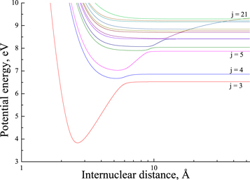
Figure 1. The SH( ) adiabatic potential energies, obtained by the asymptotic method.
Download figure:
Standard image High-resolution imageThe presently used method reproduces the long-range avoided crossings perfectly well based on the experimentally obtained atomic/ionic energy levels and the asymptotic diabatic potentials for ionic and covalent states. In some cases, ground molecular state adiabatic potentials, as well as the lowest-lying molecular state potentials are known (from experiments or ab initio calculations), so this information helps to adjust asymptotic parameters for potential curves. A comparison of model avoided crossings with available ab initio results shows good agreements. This was shown and discussed on a number of molecules treated, e.g., MgH, CaH, OH, and LiH (Belyaev et al. 2012; Mitrushchenkov et al. 2017, 2019; Belyaev & Voronov 2018). The off-diagonal matrix elements calculated by the Olson–Smith–Bauer formula might deviate from those obtained by the ab initio quantum-chemical calculations, mainly because the Olson–Smith–Bauer formula is semiempirical and provides estimates averaged over orbital angular momenta. This practically does not affect rate coefficients with large values (which are of main importance), weakly affects rates with moderate values, and remarkably affects rates with low values, but the latter rates are of low importance in NLTE stellar atmosphere modelings.
3. Sulfur–Hydrogen Collision Processes
3.1. Electronic Structure Calculations
The present investigation takes into account 55 covalent and two ionic scattering channels listed in Table 1. The atomic energy data are taken from the NIST database (Kramida et al. 2018). As mentioned above, some molecular states and/or scattering channels are omitted in the present consideration for the following reasons. (i) The two ionic molecular states have different molecular symmetries: the ground-ionic-molecular state has only the  molecular symmetry, while the first exited ionic state has three molecular symmetries:
  ,
,  , and
, and  . Figure 1 shows the potentials for the
  molecular symmetry.1
In the present study, we treat a nonadiabatic nuclear dynamics separately in each molecular symmetry, as the reaction mechanism is based on the ionic-covalent interactions. For this reason, some partial processes have negligibly low rate coefficients, if an ionic and a corresponding covalent molecular states have different molecular symmetries. (ii) The ab initio SH electronic structure calculated for the low-lying molecular states by Hirst & Guest (1982) and Vamhindia & Nsangoua (2016) indicates large energy gaps between the ground-molecular-state potential (j = 1) and the three lowest-lying excited-molecular-state potentials (
molecular symmetry.1
In the present study, we treat a nonadiabatic nuclear dynamics separately in each molecular symmetry, as the reaction mechanism is based on the ionic-covalent interactions. For this reason, some partial processes have negligibly low rate coefficients, if an ionic and a corresponding covalent molecular states have different molecular symmetries. (ii) The ab initio SH electronic structure calculated for the low-lying molecular states by Hirst & Guest (1982) and Vamhindia & Nsangoua (2016) indicates large energy gaps between the ground-molecular-state potential (j = 1) and the three lowest-lying excited-molecular-state potentials ( ), as well as other higher-lying excited-molecular-state potentials. This results in negligibly small nonadiabatic transition probabilities between these lowest-lying states and the other higher-lying states. For this reason, the scattering channel j = 1 is currently omitted. (iii) Some molecular states (e.g., the states
  ; see Table 1) have narrow nonadiabatic regions created by the long-range ionic-covalent interactions. A colliding system passes these regions almost diabatically. The resulting cross sections and rate coefficients for inelastic processes with participation of these states are negligibly low. (iv) Another reason is that corresponding molecular covalent states do not create nonadiabatic regions with an ionic molecular state, because the covalent-state potentials lie higher than the ionic-state potentials and these covalent states do not interact with ionic states within the asymptotic approach used (e.g., the states
  and some others; see Table 1). Thus, among 55 covalent and two ionic states listed in Table 1, the following adiabatic states are taken into account in the nuclear dynamical study: 13 molecular states with the
  symmetry, 42 states with the
  symmetry, 41 states with the
  symmetry, and 28 states with the
  symmetry. The results are presented below.
It should be noted that although the calculated ab initio potentials (Hirst & Guest 1982; Vamhindia & Nsangoua 2016) are low lying, they can be used to adjust model potentials to get more accurate electronic structure for the SH quasimolecule, and hence to perform more accurate calculations for the nonadiabatic nuclear dynamics.
Concerning the available ab initio SH calculations, the potentials have been computed only for the three scattering channels in S + H collisions: S(3P) + H(2S), S(1D) + H(2S) and S(1S) + H(2S). These channels generate the molecular states with the following molecular symmetries:
- 1.the ground state S(3P) + H(2S):
 , , and molecular symmetries;
 - 2.the first exited state S(1D) + H(2S):, and and
- 3.the second exited state S(1S) + H(2S):


In the present study we consider only transitions within the same molecular symmetry, so a comparison can be made only for two sets of symmetries:  and
and  . In addition, we treat only covalent states of the same molecular symmetries as the ionic states, i.e.,
  ,
,  ,
,  ,
,  . So, a comparison of the ab initio and the model nonadiabatic regions due to the ionic-covalent interaction could be performed only for one nonadiabatic region within the
  molecular symmetry, that is, a nonadiabatic region between the ground and the first-excited-molecular states. As follows from the paper (Vamhindia & Nsangoua 2016), this nonadiabatic region does not represent an avoided-crossing, in particular, because the potential of the first exited
  state is repulsive. In addition, the energy splitting between these states is relatively large,
  , so nonadiabatic transition probabilities would be negligibly small. Moreover, one nonadiabatic region between
  ab initio potential energies is not sufficient for comparison with model results. Thus, a detailed comparison of nonadiabatic regions and nonadiabatic parameters obtained by the ab initio and model approaches can not be made because of the lack of the rigorous quantum-chemical SH molecular potentials. Nevertheless, as pointed out above, we use the available ab initio potentials to adjust our model potentials to the two lowest-lying scattering channels.
3.2. Nuclear Dynamic Calculations
A nonadiabatic nuclear dynamical calculation is performed by means of the Landau–Zener multichannel approach (see Belyaev 1993; Belyaev et al. 2014; Yakovleva et al. 2016 and references therein). The Landau–Zener model is formulated as a two-coupled-state problem. When nonadiabatic regions are localized and well separated, a consequent application of the model is justified (Demkov & Osherov 1967). This takes place for relatively high-lying nonadiabatic regions because of small off-diagonal matrix elements. If multiple states interact, a consequent application can be used for estimating nonadiabatic transition probabilities as an approximation with lower accuracy than in a two-coupled-state case. Fortunately, multiple coupled states occur when the states are low lying and have large adiabatic-energy splittings. This leads to small nonadiabatic transition probabilities, low cross sections and low rate coefficients, but inelastic processes with low cross sections and rate coefficients are not important for non-LTE stellar atmosphere modeling. Thus, even rough estimates of rate coefficients for H-collision processes involving these states are sufficient.
Nonadiabatic transitions are treated separately within each molecular symmetry. The rate coefficient for the each partial process is obtained as a sum over all molecular symmetries. It should be mentioned that for mutual neutralization processes with the ground ionic state as the initial scattering channel,  (as well as for its inverse processes, the ion-pair formation), only transitions within the
  molecular symmetry contribute into the rate coefficients. For the same processes with the second ionic channel as the initial one,
  , all three molecular symmetries,
  ,
,  , and
, and  , have contributions into rate coefficients. For deexcitation/excitation processes, all four considered symmetries may have contributions.
The cross sections and the rate coefficients are calculated in the present work for the collisional energy range  and the temperature range 1000–10,000 K, respectively. The graphical representations of the calculated rate coefficients within all molecular symmetries and within the
  symmetry only are presented in Figure 2. It is seen from this figure that the inelastic processes may be divided into three groups according to their rate coefficient values:
- 1.the rate coefficients with the largest values (exceeding red squares in Figure 2);
- 2.the rate coefficients with moderate values (between 10−12 and orange, yellow, green, and light blue squares in Figure 2); and
- 3.the rate coefficients with low values (less than blue squares in Figure 2).


The first group consists of the neutralization processes:
- 1.from the first ionic state into the final states 5, 6, 7, 8, 10, and 11 (see Table 1) with values of the rate coefficients at temperature K in the range (1.08–4.48) and
- 2.from the second ionic states into the final states 48, 49, 50, and 51 (see Table 1) with values of the rate coefficients at the temperature K in the range (1.19–5.05) .


These processes are indicated by the red squares in Figure 2.
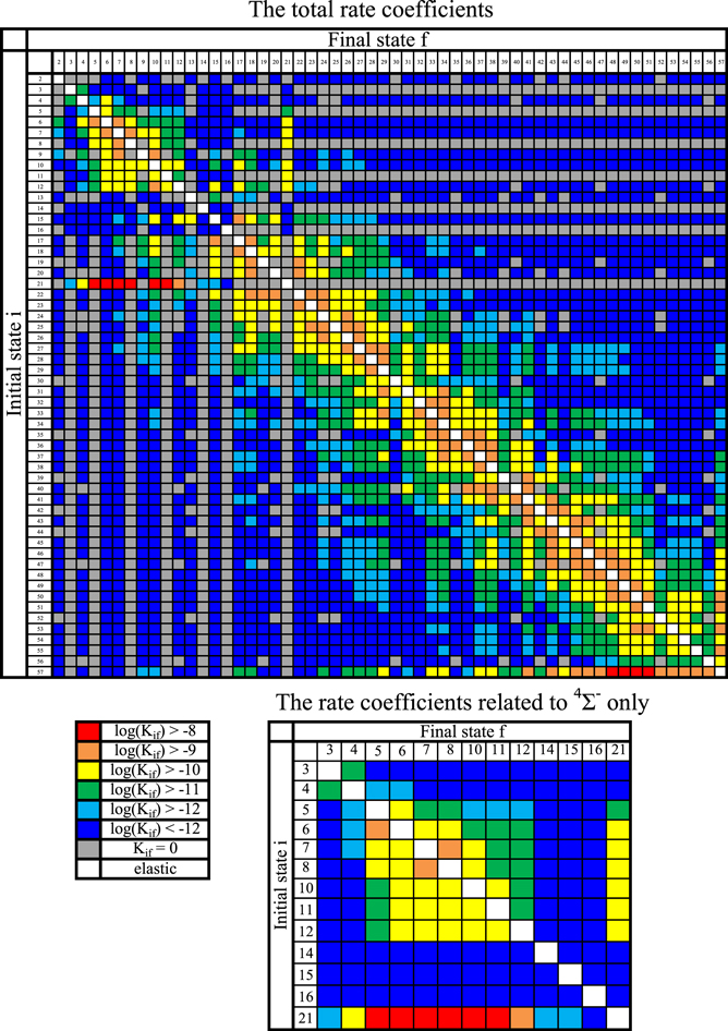
Figure 2. Graphical representation of the rate coefficients (in units  ) for partial processes of excitation, deexcitation, mutual neutralization, and ion-pair formation in sulfur–hydrogen collisions for temperature
  K.
K.
Download figure:
Standard image High-resolution imageThe second group consists of many processes of mutual neutralization, ion-pair formation, excitation, and deexcitation, especially the processes with participation of the second ionic channel. The largest values of the rate coefficients from this group correspond to the processes  ,
,  ,
,  ,
,  , and
, and  (see Table 1) with values
  , respectively, for temperature
  K. These processes correspond to the orange, yellow, green, and light blue squares in Figure 2. The processes from these two groups are likely to be important for astrophysical applications.
The third group also consists of many processes of excitation and deexcitation, as well as of a few processes of neutralization and ion-pair formation. Several important processes belong to this group, in particular,  (the transitions
  , which are related to the lines 9212/9228/9237 Å) and
  (the transitions
  , which are related to the line 8694 Å). At the temperature
  K, the rate coefficients for these processes are
  (
( ),
),  (
( ),
),  (
( ), and
  (
( ). The rate coefficients for these and other processes corresponded to the
  molecular symmetry are presented in Table 2 for temperature
  K.
K.
Table 2.
The Rate Coefficients (in units  ) for Temperature
  K for the Processes Related to the
  Molecular Symmetry
| 3 | 4 | 5 | 6 | 7 | 8 | 10 | 11 | 12 | 14 | 15 | 16 | 21 | |
|---|---|---|---|---|---|---|---|---|---|---|---|---|---|
| 3 | ⋯ | 2.03E−11 | 3.50E−14 | 1.14E−14 | 1.90E−15 | 1.68E−15 | 2.18E−16 | 1.07E−16 | 3.67E−17 | 8.20E−21 | 7.69E−21 | 4.78E−22 | 4.87E−15 |
| 4 | 6.49E−11 | ⋯ | 6.55E−12 | 1.63E−12 | 2.49E−13 | 2.18E−13 | 2.89E−14 | 1.42E−14 | 4.91E−15 | 1.05E−18 | 9.53E−19 | 4.98E−20 | 3.98E−13 |
| 5 | 1.57E−13 | 9.21E−12 | ⋯ | 8.67E−10 | 8.48E−11 | 6.71E−11 | 8.48E−12 | 4.13E−12 | 1.47E−12 | 2.62E−16 | 2.38E−16 | 1.31E−17 | 5.32E−11 |
| 6 | 1.20E−13 | 5.38E−12 | 2.04E−09 | ⋯ | 8.14E−10 | 5.56E−10 | 6.49E−11 | 3.11E−11 | 1.11E−11 | 1.40E−15 | 1.30E−15 | 8.38E−17 | 2.81E−10 |
| 7 | 2.44E−14 | 1.01E−12 | 2.45E−10 | 9.97E−10 | ⋯ | 1.78E−09 | 1.56E−10 | 7.20E−11 | 2.49E−11 | 2.72E−15 | 2.52E−15 | 1.61E−16 | 3.88E−10 |
| 8 | 1.31E−14 | 5.33E−13 | 1.17E−10 | 4.12E−10 | 1.12E−09 | ⋯ | 1.50E−10 | 6.72E−11 | 2.29E−11 | 2.30E−15 | 2.12E−15 | 1.35E−16 | 3.60E−10 |
| 10 | 4.90E−15 | 2.04E−13 | 4.26E−11 | 1.39E−10 | 2.75E−10 | 4.36E−10 | ⋯ | 1.32E−10 | 3.78E−11 | 3.04E−15 | 2.82E−15 | 1.83E−16 | 4.19E−10 |
| 11 | 8.18E−15 | 3.41E−13 | 7.07E−11 | 2.27E−10 | 4.33E−10 | 6.67E−10 | 4.56E−10 | ⋯ | 8.81E−11 | 6.15E−15 | 5.71E−15 | 3.70E−16 | 8.42E−10 |
| 12 | 5.49E−15 | 2.31E−13 | 4.89E−11 | 1.57E−10 | 2.92E−10 | 4.41E−10 | 2.53E−10 | 1.73E−10 | ⋯ | 5.12E−15 | 4.58E−15 | 3.04E−16 | 6.85E−10 |
| 14 | 4.23E−19 | 1.59E−17 | 2.64E−15 | 7.38E−15 | 1.18E−14 | 1.65E−14 | 7.59E−15 | 4.48E−15 | 1.92E−15 | ⋯ | 1.21E−18 | 6.63E−20 | 1.50E−13 |
| 15 | 7.41E−19 | 2.74E−17 | 4.46E−15 | 1.24E−14 | 1.97E−14 | 2.74E−14 | 1.27E−14 | 7.53E−15 | 3.16E−15 | 2.21E−18 | ⋯ | 1.49E−19 | 3.25E−13 |
| 16 | 2.26E−20 | 8.05E−19 | 1.25E−16 | 3.40E−16 | 5.41E−16 | 7.45E−16 | 3.50E−16 | 2.08E−16 | 8.79E−17 | 5.16E−20 | 6.40E−20 | ⋯ | 1.62E−14 |
| 21 | 4.72E−12 | 1.21E−10 | 1.15E−08 | 2.59E−08 | 3.50E−08 | 4.48E−08 | 1.84E−08 | 1.08E−08 | 4.58E−09 | 2.70E−12 | 3.20E−12 | 3.73E−13 | ⋯ |
Note. The key labels are listed in Table 1. The calculated rate coefficients are available online for the temperature range T = 1000–10,000 K.
(This table is available in its entirety in FITS format.)Download table as: ASCIITypeset image
The present study does not consider the processes related to the lines 6743–6757 Å, as these lines are determined by the transitions  . The only molecular symmetry correlated to these processes is
  , but the asymptotic energy of the state
  is higher than the asymptotic energy of the first ionic channel, so these states are not coupled by the ionic-covalent interaction treated in the approach used in the present study. Fortunately, these lines are not influenced strongly by the NLTE effects, as shown by Korotin (2009) and Korotin et al. (2017). Short-range ab initio quantum-chemical calculations of the sulfur–hydrogen quasimolecule potentials for many excited states would be helpful for studying these processes.
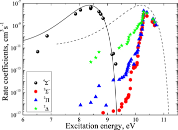
The important features are the distributions of rate coefficients between the final channels for a given initial channel. Figure 3 shows such a distribution for the mutual neutralization processes  for two initial ionic channels: S+ + H− (the ground ionic initial channel, i = 21) and
  + H− (the first-excited ionic channel, i = 57) at
  K as a function of the final-state excitation energy, which is related to the binding energy. One can see that the rate coefficients have their maximal values when the final-channel binding energy is located in the optimal window; that is, in the vicinity of −2 eV, and decrease as the final-channel excitation energies move outside the most optimal window in both directions in agreement with the prediction of the simplified model (Belyaev & Yakovleva 2017). These predictions are shown by solid and dashed lines in Figure 3. Six final channels,
  , belong to the optimal window for the mutual neutralization processes with i = 21, and four final channels,
  , for the processes with i = 57. A similar dependence, but with lower values, takes place for excitation and deexcitation processes. It is also seen in Figure 3 that the mutual neutralization within the
  symmetry (
 ) agrees better with the simplified model prediction than those within the
  ,
,  ,
,  symmetries (i = 57).
Figure 3. Mutual neutralization rate coefficients in sulfur–hydrogen ionic ( ) collisions at
  K as a function of the final-state excitation energy. Note the different initial channels (
 (ground) and
  (first-excited)) for different molecular symmetries.
Download figure:
Standard image High-resolution image
The sensitivity of the results due to small changes in the diabatic potential curves and off-diagonal matrix elements depends on a value of a corresponding rate coefficient. For the H-collision processes from the first group, the rate coefficients are stable to small changes in the diabatic potential curves and off-diagonal matrix elements; for the processes from the second group, the rates are weakly sensitive; for the third group, the rates are sensitive, but these processes are typically not important for non-LTE stellar atmosphere modelings.
4. Conclusion
In the present study, inelastic processes in sulfur–hydrogen collisions are treated by the asymptotic semiempirical approach for the potential calculation and by the Landau–Zener multichannel approach for nonadiabatic nuclear dynamics. The total number of molecular states considered is 57: 55 covalent and two ionic. The inelastic processes are treated in four molecular symmetries separately. The total number of potential energy curves computed is 128 (17 for  , 42 for
  , 41 for
  and 28 for
  ). The cross sections and the rate coefficients are calculated for the collisional energy range 10−4–100 eV and for the temperature range T = 1000–10,000 K, respectively.
It is shown that the largest values of the rate coefficients correspond to the neutralization processes 21  5, 6, 7, 8, 10, 11, and 57
  48, 49, 50, and 51, and at the temperature
  K belong to the range (1.08–5.05)
  . Many processes with moderate values of the rate coefficients correspond to the processes with participation of the molecular states with the
  ,
,  , and
, and  molecular symmetries.
Processes related to the lines 9212/9228/9237 Å and 8694 Å have low values of rates, and are equal to  (5
(5  3),
3),  (3
(3  5),
5),  (16
(16  5), and
  (5
(5  16)
16)  at the temperature
  K. The calculated data are important for NLTE stellar atmosphere modeling. The calculated rate coefficients are available online for the temperature range T = 1000–10,000 K.
The authors gratefully acknowledge support from the Ministry for Science and Higher Education (Russian Federation), projects No. 3.5042.2017/6.7 and 3.1738.2017/4.6.
Footnotes
- 1
Note that the ground-molecular-state potential is not plotted in Figure 1; see below.