


Abstract
In the vicinity of a massive black hole, stars move on precessing Keplerian orbits. The mutual stochastic gravitational torques between the stellar orbits drive a rapid reorientation of their orbital planes, through a process called vector resonant relaxation. We derive, from first principles, the correlation of the potential fluctuations in such a system, and the statistical properties of random walks undergone by the stellar orbital orientations. We compare this new analytical approach with numerical simulations. We also provide a simple scheme to generate the random walk of a test star's orbital orientation using a stochastic equation of motion. We finally present quantitative estimations of this process for a nuclear stellar cluster such as that of the Milky Way.
Export citation and abstract BibTeX RIS
1. Introduction
Most nearby galaxies possess a massive black hole (MBH) in their center, surrounded by a nuclear stellar cluster (NSC; Genzel et al. 2010; Kormendy & Ho 2013; Graham 2016). The dynamical evolution of the stellar cluster comprises numerous processes acting on different timescales (Rauch & Tremaine 1996; Hopman & Alexander 2006; Alexander 2017; see also Figure 1 in Kocsis & Tremaine 2011). Since the gravitational potential is dominated by the central MBH, stars move on nearly Keplerian orbits. The deviations from a Keplerian potential due to the stellar potential and the relativistic corrections cause the Keplerian ellipses to precess in their orbital plane. Subsequently, through the non-spherical components of the potential fluctuations, the orbital orientations of the stars get reshuffled, without changing the magnitude of their angular momentum or their Keplerian energy, through a process called vector resonant relaxation (VRR; Kocsis & Tremaine 2015 and references therein), which is the focus of this work. Resonant torques' coupling between the precessing stars then leads to a diffusion of the stars' angular momentum magnitude, a process called scalar resonant relaxation (SRR; Bar-Or & Fouvry 2018 and references therein). Finally, on longer timescales, close encounters between stars lead to the relaxation of their Keplerian energy and angular momentum (Bahcall & Wolf 1976, 1977; Lightman & Shapiro 1977; Cohn & Kulsrud 1978; Shapiro & Marchant 1978).
VRR can be a driving force behind several dynamical phenomena in galactic centers, including the warping of accretion (Bregman & Alexander 2009, 2012) and stellar (Kocsis & Tremaine 2011) disks, as well as a catalyzer of binary mergers (Hamers et al. 2018). Since its first presentation by Rauch & Tremaine (1996), VRR was studied numerically using both full (Eilon et al. 2009) and orbit-averaged (Kocsis & Tremaine 2015) numerical simulations. More recently, Roupas et al. (2017), Takács & Kocsis (2018), and Szölgyén & Kocsis (2018) studied the thermodynamical equilibria of VRR, and Fouvry et al. (2019) its axisymmetric limit.
In this paper, building upon these works, we set out to offer a detailed characterization of the VRR process in the limit of an isotropic distribution of stars. To do so, in Section 2, we present the fundamental equations of VRR. In Section 3, we characterize the properties of the potential fluctuations in the system, as inferred from estimates of the correlation function at the initial time. This will allow us to describe in Section 4 the random walk of a test particle's orientation, and develop an effective stochastic equation of motion which can efficiently mimic these random motions. Detailed comparisons of these results with numerical simulations are presented throughout these sections. In Section 5, we detail the important self-consistency existing between the potential fluctuations and the properties of the orientations' random walks. In Section 6, we use this new formalism to present the timescales associated with VRR in an NSC similar to the Milky Way's. We conclude in Section 7.
2. Model
We consider a set of N stars orbiting an MBH of mass  . On timescales longer than the in-plane precession but shorter than the time to change the orbital eccentricity (by SRR) and the time to change the semimajor axis (by two-body relaxation) the mutual interactions between two stars can be orbit-averaged over their respective mean anomalies and in-plane precession angles. As a result, each star can be replaced by a disk of mass m extending between
  = (1−e)a and
  = (1 + e)a with surface density
  =
= ![${[2{\pi }^{2}a\sqrt{r-{r}_{{\rm{p}}}}\sqrt{{r}_{{\rm{a}}}-r}]}^{-1}$](https://content.cld.iop.org/journals/0004-637X/883/2/161/revision1/apjab2f78ieqn5.gif) , where the semimajor axis a and eccentricity e can be assumed to be constant in time (see the illustration in Figure 1). Following this double orbit-average, one can associate to each star a set of conserved quantities
, where the semimajor axis a and eccentricity e can be assumed to be constant in time (see the illustration in Figure 1). Following this double orbit-average, one can associate to each star a set of conserved quantities  = (m, a, e) and a time-dependent normal vector
  , with
  the orbital angular momentum. We introduce the spherical coordinates (θ, ϕ), so that
  , with
  . Studying VRR then amounts to studying the long-term dynamics of each star's normal vector
  .
.

Figure 1. Orbit-averaged interaction between two stars orbiting a central massive object. Following the average over the fast Keplerian motion and the in-plane precession, stars are replaced by annuli, where darker colors indicate a higher surface density (not to scale). The interaction between two annuli then depends on each star's conserved parameters  = (m, a, e), as well as on their respective orbital orientations given by the normal vectors
  1 and
1 and  2.
2.
Download figure:
Standard image High-resolution imageFollowing Kocsis & Tremaine (2015), the effective single-particle Hamiltonian of VRR reads
with  (t),
(t),  i(t) the positions of the test star and the star i as they move along their (in-plane) precessing Keplerian orbits,
  the double orbit-average over these motions, and
  and Ki their respective conserved parameters. In the second line of Equation (1), we introduced the magnetizations
where the coupling coefficients  [
[ , Ki] are defined in Equation (51) below, and we used real spherical harmonics Yℓm(
 ) (defined in Equation (53)). It is also important to note that only even harmonics with ℓ ≥ 2 contribute to the particles' dynamics, by virtue of the symmetries of the interaction.
Hamilton's equations of motion read
where Lz = Lu is an action and ϕ its conjugated angle. The evolution of the angular momentum of a single test particle is given by
where the first equality is a compact rewriting of the individual equations of motion. In the second equality, we also introduced  ℓm(
ℓm( ) =
) =  × ∂Yℓm(
 )/∂
)/∂ as the real vector spherical harmonics. Because L is constant, one has
  .
.
Inspired by Klimontovich (1967), the state of the system of N stars at time t is fully characterized by the discrete distribution function (DF)

with  the Dirac delta,
  =
=  , and
, and  =
=  , with the associated volumes
  =
=  u
u  ϕ and
ϕ and 
 =
=  m
m  a
a  e. The continuity equation,
  =
= ![$-{\rm{\partial }}/{\rm{\partial }}\hat{{\boldsymbol{L}}}\cdot [\varphi \,d\hat{{\boldsymbol{L}}}/dt]$](https://content.cld.iop.org/journals/0004-637X/883/2/161/revision1/apjab2f78ieqn42.gif) , then gives us
, then gives us
where we use the fact that the vector spherical harmonics satisfy ∂/∂ ·
·  (
( ) = 0. This equation can subsequently be developed in spherical harmonics by writing

where the sum over the index α = (ℓα, mα) is implied, and we introduce

When expanded in spherical harmonics, Equation (6) becomes

where the sums over the harmonic indices (γ, δ) are implied, and we introduce the time-independent coupling tensor Qαγδ( ,
,  ) =
) =  [
[ ,
,  ] Eαγδ, with Eαγδ the (real) Elsässer coefficients (James 1973) (see Appendix B for their properties)
Equation (9) is an exact writing of the fundamental evolution equation for VRR. Its complexity stems in particular from being a quadratic matrix differential equation in the fields  .
.
All the upcoming derivations will be illustrated by comparisons with numerical simulations. In Appendix C, we present the fiducial system considered, as well as the details of our numerical implementation. In Figure 2, we illustrate a subset of trajectories from one such simulation.
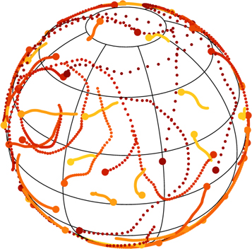
Figure 2. Random walk in orientation of a sample of particles from one fiducial simulation. The orientation of the particles is represented every 20h, with h the integration timestep (see Appendix C). Particles are colored according to their semimajor axis (from red for small a to yellow for large a). Particles with larger a see their orientation evolve more slowly, as a result of the 1/L prefactor in the interaction coefficients of Equation (51). Section 3 characterizes the properties of the potential fluctutations jointly created by this large collection of particles.
Download figure:
Standard image High-resolution image3. Correlation Function of the Noise
As a first step toward the characterization of the correlated stochastic dynamics of one star in that system, we focus on describing the properties of the density fluctuations generated as a whole by the system's N particles. In particular, we will show how one can use estimates of the derivatives of the correlation function of the density fluctuations at the initial time to provide a sensible ansatz (see Equation (22)) for the time dependences of this same correlation function.
The harmonic coefficients  (Equation (8)) describe the full state of the N-particle system (N ≫ 1) at time t and can therefore be treated as stochastic density fluctuations, assumed to be Gaussian random fields. Assuming that the system's evolution is stationary in time, the properties of these fluctuations are captured by the correlation function

where  is the ensemble average over realizations (initial conditions and trajectories of the N particles).
The correlation function is even with respect to time and generically decreases to zero on a timescale larger than some coherence time  . As a result, as a first approximation, it is therefore reasonable to replace Cαβ(
 ,
,  ', t −
  ) by a Gaussian function, tailored to match the function's behavior for t ≪
  ; see Figure 3 for a justification.
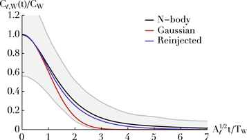
Figure 3. Correlation of the noise fluctuations, Cℓ,W ( , t), for ℓ = 2, averaged over a certain window in
  -space. The detailed parameters for this figure are spelled out in Appendix H.1. The black line is the numerical measurement, and is ensemble-averaged over 1000 realizations of the fiducial system. The background gray lines illustrate the 10% and 90% spreads over these realizations. The red line is the Gaussian prediction derived from Equation (18). The purple line is the updated prediction obtained by reinjecting the Gaussian prediction into the self-consistency relation from Equation (44), offering an exponential decay at late times.
Download figure:
Standard image High-resolution imageIn Appendix D, we compute the first two derivatives of the correlation function, and we show in Equations (64) and (68) that

and
with the coefficient

In Equation (13), we introduced n( ), the DF of the stars'
  = (a, e, m) parameters, that satisfies the normalization convention
  . We also introduced the decay rate of the correlation function Γ(
 ) as
) as

with the coefficient

Gathering Equations (12) and (13), we can approximate the correlation function  by
by

where Cℓ( , t) is a function decaying like a Gaussian:

where we introduce the torque time

Equations (17) and (18) are the main result of this section, as they provide us with a simple estimate for the time evolution of the ensemble-averaged correlation function of the fluctuations in the system. In Figure 3 we compare this estimate to the correlations measured in the numerical simulations and, to shorten the main text, we detail the procedure followed to obtain that figure in Appendix H.1. As expected, this estimation matches the numerical measurements on short timescales. Capturing the late-time, non-Gaussian behavior of the correlation function requires a self-consistent determination of the time-dependence of the noise. This is investigated in Section 5, and allows for an improved noise prediction in Figure 3. In Section 4, we will use the previous correlation functions as source terms to describe the dynamics of a test particle embedded in that noisy environment. However, in that section we will see that the ensemble-averaged correlation function does not capture the full dynamics induced on a test particle. Indeed, globally conserved quantities (such as the total energy) prevent the system from being fully ergodic: even after long times the system will not explore the entire realization space and therefore time averages are not equivalent to ensemble averages. For a given realization " ," we therefore define the time-averaged correlation function

where

stands for the time average over some long timescale T. As previously, we will assume that  (
( ,
,  ', t) can be replaced by

with the Gaussian time dependence

Here, we define the effective amplitude  (
( ) as the mean value over mα, so that
and from Equations (12), we have

which is independent of the considered harmonic. It is important to note that  varies between different realizations. In Equation (98), we illustrate how one can compute its variance, and show how this originates from the constraint of total energy conservation.
In Equation (23), we assumed, for simplicity, that the torque time,  (
( ), is independent of the considered realization. These various choices ensure that the ansatz from Equation (22) satisfies the constraints from Equations (12) and (13) when ensemble-averaged. As highlighted by Equation (22), this correlation is diagonal both w.r.t. the harmonic indices (via
  ) and w.r.t. the considered parameters (via
  (
( −
−  ')). Following Equation (23), we note that the time-dependence of this correlation is controlled by both an effective amplitude,
  , and a torque time,
  (
( ), which depend on the considered parameter
  .
.
4. Random Walk of a Test Particle
In the previous section, we characterized the noise fluctuations resulting from the coupled motions of the system's N particles. Assuming that the statistics of this noise follows the correlation function obtained in Equation (17), our goal is now to investigate the stochastic dynamics of one given test particle embedded in that fluctuating environment. In Figure 4, we illustrate one such random walk by highlighting the time evolution of the orientation of a single particle in one fiducial simulation.

Figure 4. Random walk in orientation of a given test particle from the fiducial simulations, following the same convention as in Figure 2, and represented for 0 ≤ t ≤ 104 × 20h. In Section 4, we characterize the statistical properties of that random walk on the sphere.
Download figure:
Standard image High-resolution imageThroughout this section, we use the test particle limit, i.e., we assume that the motion of the test particle is fully determined by the time-dependent density of the background particles and we neglect any backreaction of the test particle onto the background particles. We denote the parameters of the test particle with  , and its orientation at time t with
  (t). Similarly to Equation (5), the current orientation of the test particle is fully characterized by the single-particle DF:

which can be expanded as  (
( , t) = Yα(
 )
)  (with the sum over α implied), where

In practice, because the first spherical harmonics ℓ = 1 is such that  (t) ∼
(t) ∼  (t), characterizing the random walk of
  , the test particle's orbital orientation, as illustrated in Figure 4, therefore requires knowledge of the correlation properties of
  for ℓα = 1.
The evolution equation for  follows from Equation (9), and reads
where  is the harmonic coefficients of the background particles' field, as defined in Equation (8), and we introduced
  =
=  , which is a time-dependent external forcing term driving the dynamics of the test particle. The time-dependence of this source only originates from the background particles (via
  ), whose correlation properties were investigated in the previous section. We also emphasize that this forcing term also depends on
  , the parameters of the considered test particle.
Equation (28) takes the form of a time-dependent linear matrix differential equation for the test particle's harmonic coefficients  . In order to guarantee well-behaved asymptotics of the test particle's motion for large times, we approach the resolution of Equation (28) via the Magnus series (see Blanes et al. 2009 for a review). In that framework, one can generically solve for the motion of the test particle as

where the matrix Ω ( , t) is constructed as a series expansion of the form
  , whose first terms are
where [A, B] = AB − BA is the matrix commutator. As in Equation (20), for a given realization, the statistics of the motion of the test particle are captured by the stationary time-averaged correlation function

Using Equation (29), we can write this correlation function as

where we rely on our test particle's assumption (i.e., independence hypothesis; Corrsin 1959), which allowed us to separate the time average (denoted as  ) over the background particles generating the noise, and the average over the initial location of the test particle (denoted as
  ). We also rely on the hypothesis that the noise is stationary in time, so that
  , with Ω (t) ≡ Ω (0, t).
In Appendix E, we rely on the cumulant theorem to compute the two averages appearing in Equation (32). This allows us to rewrite the test particle's correlation function as
where we introduce the dimensionless function
As can be seen from the time-dependence of the exponent in Equation (33), one can note that, on short timescales, t ≪  , the correlation
  decays like a Gaussian and the motion of the particle is ballistic (e.g., (Δ
 )2 ∝ t2). On these short timescales, the random walk of the test particle is analogous to that induced by a time-independent fluctuation. On long timescales, t ≫
  , the correlation decays exponentially in time and the motion of the test star is diffusive (e.g., (Δ
 )2 ∝ t). On these long timescales, the random walk of the test particle is analogous to that induced by fluctuations
  -correlated in time (as in the classical Brownian motion), leading to a diffusive random walk on the sphere.
Because it involves an integral over  that has to be computed for every value of t, Equation (33) remains difficult to implement. Let us now present a simpler toy model to generate a stochastic motion on the sphere that would share correlation properties similar to those of Equation (33). As such, we will assume that the stochastic motion of the test particle is generated by an effective dipole Gaussian noise, and follows the Langevin equation
where the Gaussian noise  is a 3D vector of zero mean,
  , and follows
 ![$\langle {\eta }_{i}(t)\,{\eta }_{j}(t^{\prime} )\rangle ={\delta }_{{ij}}\,{e}^{-{[(t-t^{\prime} )/{T}_{{\rm{c}}}^{{\rm{t}}}]}^{2}}$](https://content.cld.iop.org/journals/0004-637X/883/2/161/revision1/apjab2f78ieqn115.gif) . We will then choose the amplitude
. We will then choose the amplitude  and coherence time
  by matching the short- and long-timescale behavior of the test particle's correlation function with the ballistic and diffusive regimes of the generic result from Equation (33), an approach already used in Hamers et al. (2018).
Following the same steps as in Equation (29), we may compute the correlation function of a test particle whose dynamics is imposed by Equation (35). It reads

with Aℓ = ℓ(ℓ + 1). By matching the ballistic and diffusive regimes of Equation (36) with those of Equation (33), we may then constrain the amplitude,  , and coherence time,
  , of the toy model of Equation (35).
The amplitude,  (
( ), varies from realization to realization and is given by

When ensemble-averaged over realizations, this amplitude becomes

as already defined in Equation (15). Finally, the coherence time is given by
where for simplicity we assume, similarly to Equation (23), that the coherence time,  (
( ), is independent of the considered realization.
Equation (36) is the key result of this section. Indeed, it provides us with an analytical description of the statistical properties of the random walk of a test particle's orientation, as jointly induced by all the background particles. The test particle's random walk is characterized by the two quantities  , which both depend on the test particle's parameters
  . On the one hand, the torque amplitude,
  , controls the amplitude of the test particle's initial ballistic motion. As such, the torque time, 1/
 , represents the typical time it would take the test particle to explore the unit sphere, for a given and frozen value of the background noise. On the other hand, the coherence time,
  , describes the typical time one has to wait for the torque amplitude to reach a statistically different value, i.e., to decorrelate itself. It corresponds therefore to the timescale after which the test particle leaves the ballistic regime to enter the diffusive regime.
One strength of the present formalism is that, following Equations (37) and (39), one now has at one's disposal explicit expressions for these two parameters. These coefficients are time-independent, and can then easily be computed for various cluster models (by varying the DF n( )) and various test particles (by varying
  ). Following Equation (36), the present approach also offers an explicit expression for the time-dependence of the test particle's correlation function,
  . Considering the same test particle as in Figure 4, we illustrate in Figure 5 one random walk generated using the Langevin Equation (35).
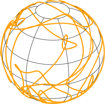
Figure 5. Random walk generated by the stochastic Equation (35) following the same convention as in Figure 4 and considering a test particle with the same  parameters.
Download figure:
Standard image High-resolution imageHowever, as we had already emphasized in Equation (22), it is important to note that the present system suffers from being non-ergodic, i.e., ensemble averages and time averages cannot be interchanged. This is highlighted by the fact that even for the exact same test particle (i.e., same  ), the amplitude
  varies from realization to realization. In Appendix F, we compute the associated variance, as given by Equation (100), and show that this effect originates from the constraint of total energy conservation. Moreover, we show that this variance remains non-zero even in the limit of a Gaussian noise, and as such does not vanish in the limit of an infinite number of background particles generating the fluctuations.
Let us finally use our fiducial numerical simulations to highlight the result from Equation (36). This is illustrated in Figure 6 and, to shorten the main text, we detail in Appendix H.2 the procedure followed to obtain that figure. In that figure we note that the numerical measurements and the analytical prediction from Equation (36) agree both on short timescales but also on timescales longer than the coherence time  (defined in Equation (118)). As already stressed in Equation (33), Figure 6 clearly exhibits the two successive regimes of evolution, namely ballistic for t ≪
  and diffusive for t ≫
  . This same figure also emphasizes the importance of accounting for the variance in
  , to correctly capture the late-time behavior of the test particles' stochastic motions. We recall that this effect that does not vanish in the limit of an infinite number of background particles. Since
  (t) ∼
(t) ∼  , Figure 6 also offers an illustration of the behavior of
  . It is also straightforward to adapt that prediction to different test stars (by changing
  ) or different galactic nuclei (by changing the DF n(
 )).
)).
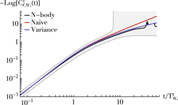
Figure 6. Correlated random walk of test particles, as captured by the correlation function,  , for ℓ = 1, averaged over a certain window in
  -space. Detailed parameters for this figure are spelled out in Appendix H.2. The black line is the numerical measurement, and was ensemble-averaged over 1000 realizations of the fiducial system. The background gray lines illustrate the 10% and 90% spreads over these realizations. The red line follows from the toy model of Equation (36). The purple line improves that prediction by accounting for the variance of
  ; see Appendix F. This figure illustrates the two successive regimes of diffusion, namely ballistic (∝t2 for t ≪
  ) followed by diffusive (∝t for t ≫
  ), as emphasized in Equation (33). The figure also highlights the importance of accounting for the variance in the amplitude
  to correct the late-time behavior of the test particles' random walks.
Download figure:
Standard image High-resolution image5. Self-consistency of the Noise
In the previous derivations, we proceeded in two successive steps. First, in Section 3, we used estimates of the derivatives of the correlation function of the noise at the initial time to obtain an ansatz in Equation (18) for the time-dependence of the correlation function of the noise generated by the N background particles. Then, in Section 4, we used this noise as a source term to study the stochastic dynamics of a test particle. Yet, if the considered test particle is taken to be one particular background particle, its random walk in orientation and the background fluctuations sourcing it have to satisfy some self-consistency relation. This is what we explore in this section.
We start from Equation (20), and replace  by its definition in terms of a discrete sum over particles, as in Equation (8), so that
We now assume that each background particle can be treated as a test particle, and that their long-term motions are decorrelated one from another. Only contributions from i = j remain, and Equation (40) becomes

where  is the test particle's correlation function of the particle i, as defined in Equation (31). To proceed further, let us now take the ensemble average of both sides of Equation (41), to get

Luckily, in Equation (32), we have already solved for the correlation function of the random walks of the test particle through the Magnus series. Using Equation (74), we generically obtain
We may then take the ensemble-average of this relation and, for simplicity, keep only the first cumulant in the cumulant theorem. Reinjected into Equation (42), this leads to
Equation (44) takes the form a self-consistent integral equation satisfied by the correlation of the noise fluctuations in the system. This relation can be further clarified by defining

and one finally gets the self-consistent differential equation4
Equation (46) is the important result of this section, as it highlights the self-consistent relation satisfied by the correlation of the noise fluctuations. Yet, as it couples both different harmonics (via  ) and different parameters (via
  ), such a differential equation appears too intricate to easily be solved explicitly. This is not pursued further here.
One may still proceed iteratively to obtain improved approximations of the noise correlation function. To do so, one starts from the Gaussian dependence obtained in Equation (18). This (motivated) ansatz may then be reinjected in the rhs of the self-consistency relation from Equation (44), leading to a new expression of the noise correlation function that would have both a ballistic and a diffusive part. Such a procedure is illustrated in Figure 3, where we show how one can better match the late-time properties of the system's noise through this iterative process.
6. Application
As an illustration of the present formalism, let us now consider the case of a stellar cusp distribution similar to that of SgrA*. The mass of the MBH is taken to be  = 4 × 10⁶ M⊙, and for simplicity we consider a single-mass stellar population of individual mass m⋆ = 1 M⊙. We assume that the stars' eccentricities follow a thermal distribution, fe(e) = 2e (Merritt 2013), and that the number of stars per unit a follows a power-law distribution of the form
  , where N0 = g(γ)N(<a0), with

and N(<a0) the physical number of stars within a sphere of radius a0 from the center. For the numerical application, we assume that a0 =  = 2
= 2  and N(<a0) = 4 × 10⁶. The system being of infinite extent, we write the system's DF as n(m, a, e) = fm(m)fe(e) na(a)/(4π).
In Appendix I, we show that the amplitude Γ2, defined in Equation (15) and characterizing the ballistic regime of the orientation's random walk, follows the power-law distribution
where P(a) = 2π(a3/ is the orbital period, and
  is a dimensionless eccentricity function defined in Equation (127) and illustrated in Figure 10. In Figure 7, we illustrate the dependence of the torque time, 1/Γ, for circular orbits of different semimajor axes and for different cusp profiles, and interestingly note that this VRR timescale is similar to the age of some of the young stars observed in our Galactic center (Habibi et al. 2017).
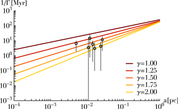
Figure 7. Torque time, 1/Γ, for circular orbits (e = 0) as a function of the semimajor axis, and for different cusp profiles (through the power index γ) similar to that around SgrA*. For comparison, black circles with errors show the main-sequence ages of the subset of S-stars whose age was recently estimated in Habibi et al. (2017).
Download figure:
Standard image High-resolution imageAs shown in Figure 7, should the S-stars be born in a disk, the VRR process is sufficiently fast to isotropize their orbital orientations (Hopman & Alexander 2006), but SRR may not be efficient enough to thermalize their eccentricities (Bar-Or & Fouvry 2018).
One can follow a similar calculation to obtain the expression of the coherence time,  , defined in Equation (39) and characterizing the diffusive regime of the orientation's random walk. It follows the power-law distribution
where the dimensionless eccentricity function fT (e) is given in Equation (132) and illustrated in Figure 10. In that figure, we note that for a thermal eccentricity distribution and a cusp's power index 1 ≤ γ ≤ 2, one can assume that  , which leads to the torque time and the coherence time following the approximate relation
We note that this simple relation allows for an even simpler generation of samples of random walks in orientations as given by the toy model from Equation (35), as one only has to estimate the test particle's torque time 1/Γ (a, e), as the associated coherence time,  (a, e), follows immediately.
7. Conclusion
In the present work, we illustrated how one can describe quantitatively the statistical properties of the stochastic evolutions of star's orientations in galactic nuclei during the process of VRR. The main difficulty in the present derivation lies in the system being fundamentally degenerate, i.e., having a vanishing mean field Hamiltonian, H = 0. This system is also non-Markovian, i.e., correlated in time, as well as non-ergodic, i.e., time- and ensemble-averages cannot be interchanged.
Placing ourselves in the limit of an isotropic distribution of stars, we circumvented some of these difficulties in Section 3 by assuming that the statistical properties of the noise fluctuations can be derived from estimates of the derivatives of their correlation function at the initial time. The main result was obtained in Equation (22), which provided us with a self-consistent ansatz for the statistical properties of the time-dependence of the correlation of the fluctuations generated jointly by the system's N particles. In Section 4, we used this result to describe the random walk of a test particle's orientation embedded in this stochastic system, recovering both the ballistic and diffusive regimes. The main result was obtained in Equation (36), which yields quantitative predictions for the statistical properties of that random walk. The key tools used at that stage were the Magnus series to solve the linear matrix evolution equation for the test particle, the independence hypothesis to separate the statistics of the background noise from that of the test particle's random walk, and the cumulant theorem to estimate ensemble averages. We also emphasized how non-ergodic effects (associated with the constraint of total energy conservation) should be accounted for to allow for reliable long-timescale predictions. Throughout the text, all the predictions were compared with detailed numerical simulations offering a quantitative agreement. In Section 5, we highlighted the self-consistency existing between the spontaneous fluctuations in the system and the associated random walks in orientations. Finally, in Section 6, we presented a first application of this framework to estimate the timescales of VRR in a stellar cusp similar to that of SgrA*.
This paper is only a first step toward a complete theory of VRR, and we list below some possible avenues for future development. In the current derivation, we relied extensively on the isotropic assumption, and as such neglected any effects associated with anisotropic clustering in orientation (Szölgyén & Kocsis 2018). For binaries, the exact statistical properties of the VRR random walk in orientation can lead to enhanced rates of mergers (Hamers et al. 2018), hence the importance of quantitative predictions for the properties of these random walks, as obtained in Equation (36). Building upon Section 4, one could also investigate how a substructure like a disk stochastically dissolves (Kocsis & Tremaine 2011). This asks for a detailed accounting of the correlations in the potential fluctuations of a given realization, to characterize how stars with similar initial orientations or similar parameters get slowly separated. Finally, here we focused our interest on systems dominated by a central mass. Provided one updates accordingly the interaction coupling coefficients,  [
[ ,
,  ], similar investigations could be pursued in the context of spherical globular clusters (Meiron & Kocsis 2018).
We thank Christophe Pichon and Scott Tremaine for remarks on an earlier version of this manuscript. J.B.F. acknowledges support from Program number HST-HF2-51374 which was provided by NASA through a grant from the Space Telescope Science Institute, which is operated by the Association of Universities for Research in Astronomy, Incorporated, under NASA contract NAS5–26555. B.B. is supported by membership from Martin A. and Helen Chooljian at the Institute for Advanced Study.
Appendix A: Coupling Coefficients
Similarly to Equation (10) in Kocsis & Tremaine (2015), we define the coupling coefficients5
where ![$L[{\boldsymbol{K}}]=m\sqrt{{{GM}}_{\bullet }a(1-{e}^{2})}$](https://content.cld.iop.org/journals/0004-637X/883/2/161/revision1/apjab2f78ieqn169.gif) is the magnitude of the angular momentum. We also introduce "out" (resp. "in") as the index i or j with the larger (resp. smaller) semimajor axis, and define accordingly the ratio α =
is the magnitude of the angular momentum. We also introduce "out" (resp. "in") as the index i or j with the larger (resp. smaller) semimajor axis, and define accordingly the ratio α =  /
/ ≤ 1. With this notation, the dimensionless coefficients sℓ[α,
  ,
,  ] are given by
with Pℓ(u) the usual Legendre polynomials. Because they are independent of the details of the considered system, the coefficients sℓ[α,  ,
,  ] can be precomputed on a grid to hasten the numerical evaluation of
  [Ki, Kj]. For our fiducial simulations, these coefficients were pre-computed on a linear 3D grid in (α,
  ,
,  ) consisting of 2003 elements, with 10−2 ≤ α ≤ 1 and 0 ≤
  ,
,  ≤ 0.99. We refer to Figure 1 in Kocsis & Tremaine (2015) for an illustration of the behavior of these coefficients.
Appendix B: Elsässer Coefficients
In this appendix, we follow James (1973) and Ivers & Phillips (2008) and detail some of the properties of the Elsässer coefficients. We emphasize that we work with real spherical harmonics, hence the need for some identities to be adapted.
The real spherical harmonics are defined with the convention
with  (u) the usual associated Legendre polynomials, and the coefficients
 ![${K}_{{\ell }}^{m}={\left[\tfrac{2{\ell }+1}{4\pi }\tfrac{({\ell }-m)!}{({\ell }+m)!}\right]}^{1/2}$](https://content.cld.iop.org/journals/0004-637X/883/2/161/revision1/apjab2f78ieqn182.gif) . With this convention, the spherical harmonics follow the normalization
. With this convention, the spherical harmonics follow the normalization  =
=  .
.
Following Equation (5.5) of Ivers & Phillips (2008), the real Elsässer coefficients, as defined in Equation (10), can be decomposed as

where  only depends on (ℓα, ℓγ, ℓδ), while
  also depends on (mα, mγ, mδ). The m-independent coefficients read
where we introduce the Wigner 3j-symbols (Arfken et al. 2005), and define
The coefficients  are given by
where the tensor  comes from the fact that we are considering real spherical harmonics, and is given by
The Elsässer coefficients satisfy various exclusion rules (James 1973). In particular, for Eαγδ to be non-zero, one has to satisfy
These coefficients also follow the symmetry relations Eαδγ = Eγαδ = −Eαγδ.
Finally, following Varshalovich et al. (1988), the Elsässer coefficients satisfy various contraction identities. In particular, throughout the derivations, we will rely on
Appendix C: Numerical Simulations
In this appendix, we briefly detail the numerical simulations to which our analytical results are compared. To simulate a system of N interacting particles, the starting point is the evolution Equation (4), that can be used for each of the N particles. In that form, we note that the velocity vector,  /
/ t, is expressed only as a function of the current location of the particle,
  i(t), and the instantaneous particle's magnetizations, Mℓm (Ki, t). There are N such evolution equations, but because the magnetizations vary from one particle to another, their computation has to be made once per timestep and particle. As a result, the overall complexity of advancing the particles for one timestep scales like
  , with ℓmax the maximum harmonic number considered in the pairwise interaction.6
In our approach, the motion of the particles is integrated by computing the magnetizations, while in the implementation presented in Kocsis & Tremaine (2015), particles are moved forward by solving successively pairwise interactions, an approach symplectic by design. The method of Kocsis & Tremaine benefits from parallelization by computing the pairwise interactions in parallel, provided that they are carefully ordered; see their Section 3.2. The present approach benefits from parallelization when computing the
, with ℓmax the maximum harmonic number considered in the pairwise interaction.6
In our approach, the motion of the particles is integrated by computing the magnetizations, while in the implementation presented in Kocsis & Tremaine (2015), particles are moved forward by solving successively pairwise interactions, an approach symplectic by design. The method of Kocsis & Tremaine benefits from parallelization by computing the pairwise interactions in parallel, provided that they are carefully ordered; see their Section 3.2. The present approach benefits from parallelization when computing the  magnetizations, seen as a contraction of large matrices and vectors.
Our numerical implementation proceeds then by (i) computing efficiently the spherical harmonics (and the vector ones) at the location of the particles, (ii) computing the magnetizations in Equation (2), (iii) computing the velocity fields in Equation (4), and (iv) advancing all the particles' orientation for one timestep. The real spherical harmonics are computed using a recurrence relation for the renormalized associated Legendre polynomials (see Equation (6.7.9) in Press et al. 2007), and using the second-order recurrence relation  (similarly for sin(m ϕ)) for the azimuthal component. To compute the real vector spherical harmonics, we follow the same recurrence as in Appendix B.2 of Mignard & Klioner (2012), adapted to the renormalized associated Legendre polynomials. Once all the velocity vectors
  /
/ t are computed, particles are advanced for a timestep h, using a fourth-order Runge–Kutta integrator (see Equation (17.1.3) in Press et al. 2007).
All the derivations presented in the main text are illustrated with comparisons using this numerical approach. We consider a system composed of N = 103 stars, and assume that the particles' conserved quantities Ki = (mi, ai, ei) satisfy m =  ,
,  ≤ a ≤
≤ a ≤  , and
, and  ≤ e ≤
≤ e ≤  . Our units are chosen so that
  =
=  = G = 1, and we pick
  /
/ = 100,
  = 0, and
  = 0.3. These parameters are drawn independently one from another, according to probability distribution functions (PDFs) proportional to (
 (m −
(m −  ), a1/2, e), which corresponds to a single-mass population in a harmonic profile with a thermal distribution of small eccentricities. The stars' initial orientations are drawn uniformly on the sphere, and the interactions are truncated at ℓmax = 50. The timestep of the simulation is the same for all particles and is determined at the start of each realization. To do so, we compute the torque exerted on every particle at the initial time,
  , and define
  as the associated torque time. The integration timestep is then fixed initially to
 ![$h={10}^{-2}\times {\mathrm{Min}}_{i}[{t}_{\tau }^{i}]$](https://content.cld.iop.org/journals/0004-637X/883/2/161/revision1/apjab2f78ieqn215.gif) . With such choices, integrating the system for one timestep takes approximately 1 s on a single core, and simulations are carried out for 2 × 10⁵ timesteps.
. With such choices, integrating the system for one timestep takes approximately 1 s on a single core, and simulations are carried out for 2 × 10⁵ timesteps.
Appendix D: Computing the Derivatives of the Noise Correlation
D.1. Computing Ensemble Averages
We are generically interested in computing ensemble averages at the initial time of the form  . Such averages can be carried out explicitly by noting that, at the initial time, the N particles are drawn independently one from another, both for their orientations and their parameters. Following our isotropic assumption, their orientation is drawn uniformly on the sphere, according to the PDF f (
 ) = 1/(4π), while we assume that their parameter
  is drawn according to a PDF g(
 ), normalized so that
  .
.
To illustrate the gist of these calculations, let us consider the case  . As they do not contribute to the dynamics, we never need to consider the harmonics (ℓ, m) = (0, 0), so that
  . Owing to the particle independence at the initial time and following the definition from Equation (8), we can write
where non-zero terms only come from i = j, and we introduce the connected average as
When considering averages at the initial time involving more than two fields, we limit ourselves to the dominant contributions associated with pair couplings (i.e., the limit of Gaussian fields, Wick's theorem). We can then write
where "perm" browses all the possible pair decompositions without repetitions, and averages involving an odd number of fields are neglected.
D.2. Initial Values of the Correlation Function
Following the method just described, we may now estimate the value and the second derivative of the correlation function at the initial time, as introduced in Equation (11).
For the value at the initial time, we can write

where we follow Equation (61) to compute the last average, and introduced n( ) = g(
 ) N/(4π) as the DF of the stars' parameters satisfying the normalization
  . We emphasize that to compute Equation (64), we relied on the assumption of an isotropic distribution of particles on the sphere, which led to the Kronecker coefficients
  w.r.t. the harmonic coefficients.
The ensemble average expectation for the first derivative at the initial time reads  =
=  ∼
∼  , where we used the quadratic evolution Equation (9) once. As it involves an odd number of fields, this correlation is equal to zero, as imposed by Equation (63).
Let us now turn to the computation of the ensemble-average expectation for the second derivative of the correlation at the initial time. We write
where we inject the evolution Equation (9) twice. As shown in Equation (63), in the limit of Gaussian fluctuations, the average term can be computed by keeping only averages of pairs. As Eαγγ = 0, only two of the possible couplings remain, namely 
 and
and 
 , which leads to
where we use Eβδγ = −Eβγδ, and introduce
Following Equation (60), one can now perform the sums over mγ and mδ in Equation (66). The VRR interactions being limited to even harmonic numbers ℓ, we may impose at this stage that ℓα is even. Glancing back at the constraint {C2} from Equation (59), we note that ℓα + ℓγ + ℓδ has to be odd, so that the term Λγδ( ,
,  ') never contributes to Equation (66). For ℓα even, Equation (66) becomes

where the sum over ℓδ is performed following Equation (60), and the decay rate Γ2 ( ) is given by Equation (15).
Appendix E: Computing the Properties of the Random Walk
In this appendix, we compute the two averages appearing in Equation (32). Assuming that the test particle is initially uniformly distributed on the sphere, one straightforwardly has
To compute the time average of  Ω (t), we rely on the cumulant theorem,
where  are the moment matrices, and κn are the cumulant matrices, with the first two given by κ1 = μ1 and
  . Here, we compute the time average of
  Ω(t) by keeping only terms that are at most second order in
  , so that only
  and
and  contribute. We note that since
  and, from stationarity,
  , both
  and
and  vanish. As a result, at the order considered here, only the second cumulant
  is non-zero, and from the cumulant theorem we obtain

Gathering Equations (69) and (71) together, we can write the test particle's correlation function as

Using Equation (30), we can write
To pursue the calculation further, we may now use our ansatz for the time-dependence of the correlation of the noise fluctuations, as obtained in Equation (22). Using the sum identities from Equation (60), one gets
where  is a double time integral of the noise correlation
with the dimensionless function χ (τ) defined in Equation (34). Since the matrix  is diagonal, one can straightforwardly compute its exponential, as required by Equation (71). This allows us to finally recast the correlation of the test particle's random motion from Equation (72) under the form of Equation (33).
Appendix F: Computing the Variance of the Noise Amplitude
In this appendix, we compute the ensemble-averaged variance of the amplitude of the density fluctuations,  , as introduced in Equation (20). Our goal is to compute an expression of the form
Because only even harmonics contribute to the interactions, we can limit ourselves to 2 ≤ ℓα, ℓγ even. As estimated in Equation (23), we know that for  , the location of the background particles at time
  can be considered to be decorrelated from their locations at time t, up to the requirement of satisfying the system's global conservation constraints. It is fundamental to account for these global conservation constraints, as they introduce non-ergodic effects, preventing us from interchanging time- and ensemble-averages. Provided that these constraints are satisfied, in the two-dimensional time integral from Equation (76), one can note that the particles are uncorrelated between t and
  on a surface of size (T −
  )2, while they are correlated on a surface of size T
  . As a result, as long as T ≫
  and as long as the conservation constraints are satisfied, particles can be considered as uncorrelated between time t and
  , and therefore distributed uniformly over the sphere at these two times.
Let us now detail how one may carry out the average from Equation (76), in the presence of these constraints. At time t, the state of the system is fully characterized by the set of all fields  and, similarly, at time
  , the state of the system is fully characterized by
  = {
= { }. We may then use
  and
and  as the random variables over which averages are carried out. Following Equation (12), we have
and similarly for  . Placing ourselves within the Gaussian limit, we may then treat
  (resp.
  ) as uncorrelated Gaussian random fields that follow a Gaussian PDF F (
 ) (resp. F (
 )), with a covariance following from Equation (77).
As emphasized above, the two fields  and
and  remain correlated one with another through global constraints. To shorten the notation, let us temporarily denote these constraints as
  =
=  (
( ). In Equation (76), the average must then be carried out according to the joint PDF
  . The conditional PDF of
  given the constraint
  (
( ) follows from Bayes' theorem, and reads

with  the PDF of the constraints
  . Therefore, we can write
In that view, Equation (76) can be recast as
where we introduce
with  standing for the ensemble average where the fields
  are drawn according to the Gaussian statistics of F(
 ). Conveniently, in that form, Equation (80) allows us to carry out independently the averages over
  and
and  .
.
To proceed further, let us now detail the global conservation constraints that have to be satisfied throughout the system's evolution. There are three such constraints, namely the conservation of each particle's individual parameters ( 0), the conservation of the system's total angular momentum (
 1), and the conservation of the system's total energy (
 2). Luckily, these can all be expressed as simple functions of the fields
  . They read
with ![$L[{\boldsymbol{K}}]=m\sqrt{{{GM}}_{\bullet }a(1-{e}^{2})}$](https://content.cld.iop.org/journals/0004-637X/883/2/161/revision1/apjab2f78ieqn290.gif) the norm of the angular momentum and Hℓ[
the norm of the angular momentum and Hℓ[ ,
,  ] = L [
 ]
]  [
[ ,
,  ]. We also note the prefactor 1/(2N) in the definition of the energy that was introduced for later convenience. At this stage, it is important to note that each of these constraints involve different harmonics of the Gaussian random fields, namely ℓ = 0 for the conservation of
  , ℓ = 1 for the angular momentum, and 2 ≤ ℓ even for the energy. In the limit of Gaussian random fields, this implies that only the energy constraint contributes to a non-zero variance in Equation (80), as we will now argue.
Since only even harmonics contribute to the interactions, we can restrict ourselves to 2 ≤ ℓα even when computing  . If ℓβ = 0, 1, Equation (81) can be rewritten as
where we used the Gaussian assumption, so that fields with different harmonics are uncorrelated. Because the energy is quadratic in the fields, and because the Gaussian PDF, F( ℓ≥2), is an even function of the fields, the last bracket in Equation (83) is equal to zero. As a result, we can assume that ℓβ ≥ 2. In that case, Equation (81) becomes
where we introduce

As a result, for ℓα, ℓβ, ℓγ, ℓδ ≥ 2, this allows us to rewrite the required correlation from Equation (80) as
where we get rid of all occurrences of the constraints  0 and
0 and  1, using the fact that their PDFs satisfy
  . As a conclusion, in the limit of Gaussian random fields, only the constraint of total energy conservation contributes to the non-ergodic properties of the system. This is an important result of this calculation.
Let us now compute the ensemble average appearing in Equation (85). In the present Gaussian limit, we can rely on Novikov's theorem (Novikov 1965) to compute it.7 One obtains
where the first cumulant is absent because ℓα ≥ 2, so that  , and only the second cumulant remains as the fields are assumed to be Gaussian. In Equation (87), the sum (resp. integral) over μ (resp.
  ) runs over all the fields. The functional gradient appearing in the last term can be computed as
where we use the fundamental relation 
 /
/
 =
=  − Kμ). Glancing back at the definition of the energy in Equation (82), we can also write
Injecting these results into Equation (87) and using the Gaussian statistics from Equation (77), we obtain a self-consistent integro-differential equation for  αβ
αβ , Kβ, E), namely
where we use that  = FE (E), by definition.
Progress can now be made by accounting perturbatively for the total energy constraint. As such, we introduce the small parameter  , make the substitution Hℓ →
  Hℓ in Equation (90), and consider the expansion

We can then inject this expansion in Equation (90) and match the orders in  . The first three terms are obtained as
Owing to these first terms, we can now return to the computation of the variance from Equation (86). Keeping only terms of at most second order in  , this reads
where, for simplicity, we do not repeat the arguments  , Kβ) and
  , Kδ). The zeroth-order term is straightforward to compute, and gives
using  . It is straighforward to show that the first-order term satisfies

as the energy integrals vanish. Using a similar argument, one finds that terms of the form  (0)
(0)  (2) do not contribute to the second-order term in Equation (93). Keeping only the non-zero contribution coming from
  , we get
where ΔE is obtained after straightforward manipulation of the energy integrals, and reads
It is important to note that ΔE is a single number that depends only on the total energy PDF, FE (E), and therefore only on the considered DF n( ). In Appendix G, we detail how the required integral from Equation (97) can be estimated. Equation (96) is an important result of this appendix, as it characterizes the variance (over different realizations) of the noise fluctuations' amplitude arising from the constraint of total energy conservation.
Following Equation (24), we can get the variance of  (
( ). It reads

where we introduce the dimensionless function Mℓ( ) as
) as

The final step of this appendix is to compute the variance of  , as defined in Equation (37). We get
with  =
=  − Γ2. Equation (100) is the final result of this section. It expresses the variance (over realizations) of
  , the amplitude of the random walk of a given test star. It is important to note that since (Γ2)2 and
  have the same scaling with N, the present variance effect does not vanish as the number of particles gets larger.
As it will be needed to obtain the prediction of Figure 6, let us illustrate the effect associated with this non-zero variance of  in our fiducial simulations. We consider the same window,
  (
( ), as in Equation (115). For each test particle falling in that window, we measure the correlation function
  (e.g., for ℓα = 1). The second-order time derivative at t = 0 of this correlation function is directly proportional to
  (see Equation (36)), which we can therefore measure numerically. In Figure 8, we represent the distribution of these numerically measured initial values,
  , and illustrate how these amplitudes vary from realization to realization.
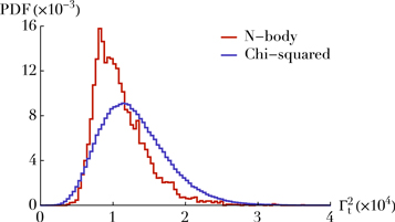
Figure 8. Variation in  for the test particles falling in the same window
  (
( ) as in Figure 6. The red histogram is the distribution of
  measured over 1000 realizations. This distribution is characterized by
  and
and  . The purple histogram has been obtained via a resampling of
  following chi-squared distributions with means and variances predicted in Equations (37) and (100). This distribution is characterized by
  and
and  ≃ 7.7.
Download figure:
Standard image High-resolution imageTo capture this variance effect seen in Figure 8, we may use our estimation of the variance of  obtained in Equation (100). To do so, for every test particle falling in the window, we compute
  , following Equations (38) and (100). Having determined this mean and variance, one can draw a sample of
  according to a PDF that shares the same first two cumulants. Similarly to Equation (105), we assume that we can draw this sample according to a chi-squared PDF with these imposed mean and variance. The result of this procedure is illustrated in Figure 8. This figure illustrates how the present calculations are able to capture most of the features associated with the non-vanishing variance of the test particles' individual amplitudes
  .
.
Appendix G: Computing the Variance of the Energy Distribution
In this appendix, we briefly detail how one can estimate the energy spread ΔE introduced in Equation (97). Our convention for the definition of the total energy is spelled out in Equation (82). Using the two-point statistics from Equation (62), the expected mean value of the energy reads
where we define

We can proceed similarly to compute the expectation for  . This reads
To compute the average term appearing in the rhs, we follow Equation (63), placing ourselves in the limit of Gaussian random fields so that only connected averages involving two fields remain. We get
where we use the symmetry relation Hℓ[ ,
,  ] = Hℓ[
 ,
,  ], and introduce

Having estimated the mean and the variance of the energy distribution, we may now return to the evaluation of the energy spread ΔE introduced in Equation (97). As the energy is a quadratic function of Gaussian fields, we will assume that it follows a (scaled) chi-squared distribution of mean μ =  , and variance
  . The associated PDF then follows
with κ = μ2/σ2. For our fiducial numerical system, we find  ≃ 6.1 × 10⁻³ and κ ≃ 81. In Figure 9, we illustrate the statistical distribution of the system's energy, as well as the approximation from Equation (106).
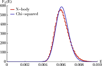
Figure 9. Statistical distribution of the system's total energy. The red histogram has been estimated numerically by computing the initial energy of 2 × 10⁵ realizations. This histogram is characterized by  ≃ 6.1 × 10⁻³ and
  ≃ 65. The black line corresponds to the chi-squared PDF prediction from Equation (106), for which
  and κchi ≃ 81.
Download figure:
Standard image High-resolution imageFinally, for a chi-squared PDF as in Equation (106), one can explicitly compute ΔE, as defined in Equation (97), to get

We note that this integral is well-behaved only for κ > 2. This is an artefact coming from the perturbative expansion introduced in Equation (91). For our fiducial model, we find ΔE ≃ 6.7 × 10⁻⁴.
Appendix H: Computing Averages over a Window
In this appendix, we briefly detail the procedures used in Figures 3 and 6 to compare our analytical results with the fiducial numerical simulations.
H.1. Correlation of the Noise Fluctuations
Let us detail the method followed to obtain Figure 3, used to illustrate Equation (22). One of the key insight from this equation is that to any particle (of parameter  ), we can associate the pair (n(
 ),
),  (
( )) that characterizes the correlation properties of the density fluctuations generated by background particles with these parameters. As a result, in order to consider only particles that have similar noise decorrelation properties, it is convenient to introduce, for every realization, the
  -averaged fields
  , with W(
 ) a window function defined8
as
) a window function defined8
as
with (Cmin,  ) the typical amplitude and torque time considered, and
  W a small dimensionless parameter controlling the size of the window. We then naturally have
  , with the sum limited to the particles with (n(
 ),
),  (
( )) in the vicinity of (Cmin,
  ). Introducing
  (t −
(t −  ) ≡
) ≡  , Equation (22) immediately gives

where the function  (
( , t) follows the Gaussian ansatz from Equation (23). When averaged over realizations, Equation (109) can be approximated with the Gaussian dependence

where we introduce the amplitude CW and torque time TW as
Equation (110) is the analytical Gaussian prediction illustrated in Figure 3.
In Figure 3, we also present an updated prediction of the noise correlation obtained by reinjecting the Gaussian prediction from Equation (18) into the self-consistency relation from Equation (44). In that context, when averaged over the window, the prediction takes the form
with CW as in Equation (111), and where the amplitude  and coherence time
  are given by

In these equations, we introduce  as the mean over the window W(
 ), i.e., it is defined as
We illustrate such measurements in Figure 3. As defined in Equation (108), we chose the window W( ) with the parameters (Cmin,
  ) ≃ (5.0, 142), with
  W = 0.1. With such a choice, there are on average nine particles in the window per simulation. Following Equation (111), the typical amplitude and torque time in the window were found to be (CW, TW) ≃ (0.72, 148).
H.2. Correlation of the Random Walks
Let us briefly detail the method followed to obtain Figure 6, used to illustrate the result from Equation (36). Following the independence hypothesis from Equation (32) we assume that, for a given realization, each individual particle can effectively be treated as a test particle. As such, we neglect the correlations existing between the background fluctuations and the random walk of that particular particle.
One important insight from Equation (36) is that to any test particle (of parameter  ), we can associate the pair (Γ2(
 ),
),  , that characterizes the correlation properties of its random walk in orientation. Similarly to Equation (108), in order to investigate these random walks, it is convenient to introduce the window function
  (
( ) as
) as
where ( ,
,  ) are the typical amplitude and coherence time of the considered test particles, and
  is a dimensionless parameter controlling the size of the window. We may then define the window-averaged correlation function (which can easily be measured in the numerical simulations) as

where  stands for the mean over the test particles of a given realization falling in the window
  (
( ), similarly to Equation (114). Following Equation (36), we also add a prefactor 4π to ensure that this correlation is between 0 and 1.
If one does not account for the variance in  (see Equation (100)), a first (naive) prediction for Equation (116) can be obtained from Equation (36) by restricting ourselves only to the ensemble-averaged mean predictions. This gives
where the amplitude,  , and coherence time,
  , are computed by direct averages over the particles falling in the window
  (
( ), so that

One can improve the prediction from Equation (117) by accounting for the variance in  . To do so, for every test particle falling in the window, one can compute the mean expectation for the amplitude,
  , and the associated variance,
  , as given by Equations (38) and (100). For this same particle, one can then draw an effective value of
  , according to a chosen PDF with this prescribed mean and variance. This process is illustrated in Figure 8, where we used a chi-squared PDF. In that case, the prediction from Equation (117) becomes
Here, the amplitude and coherence time from Equation (118) become

where PDF [μ, σ2] returns a sample from a chosen PDF of mean μ and variance σ2 (which we chose to be a chi-squared PDF as in Figure 8).
We illustrate such measurements in Figure 6. As defined by Equation (115), we chose the window  (
( ) with the parameters
  and
and  . Following Equation (118), the typical amplitude and coherence time in the window were found to be
  .
.
Appendix I: Case of a Power-law Distribution
In this appendix, we detail all the calculations presented in Section 6 for an infinite power-law stellar distribution around an MBH. We first note that the squared coupling coefficients from Equation (51) can be rewritten as
where we recall that "out" (resp. "in") labels the star with the larger (resp. smaller) semimajor axis, and we introduced the dimensionless ratio α =  /
/ .
.
Following Equation (15), we can then compute the amplitude, Γ2, of the background fluctuations. It reads
where we introduce the second moment of the mass distribution  . The integral over
  in Equation (122) can then be split into two regions,
  ≤ a and
  ≥ a. For the first region, we write
and a very similar calculation can be carried out for the second region to get
In order to shorten the notation, let us introduce the dimensionless integrals
where one should pay attention to the order of the arguments of  . This allows us then to rewrite Equation (122) as
where we introduce the amplitude Γ0 and the dimensionless function  as
as
In Figure 10, we illustrate the dependence of  , assuming a thermal eccentricity distribution, fe(e) = 2e, and different cusp profiles. We also note that Equation (127) is essentially identical to the result already presented in Equation (D5) of Kocsis & Tremaine (2015).
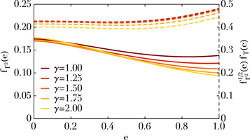
Figure 10. Dimensionless eccentricity functions  (left axis, full lines) and
  (right axis, dashed lines), for different cusp profiles (through the power index γ) and assuming a thermal eccentricity distribution,
  . We note that
  independently of e and γ. Calculations of the integrals over α were performed using the same grid in sℓ as in Appendix A.
Download figure:
Standard image High-resolution imageLet us now pursue a similar approach to compute the coherence time,  , as introduced in Equation (39). When expanding the rhs of that equation, one gets
The integral over da' can be carried out following the same approach as in Equations (123) and (124) to get
Similarly to Equation (125), in order to shorten the notation, we define the dimensionless integrals
where once again, one should pay attention to the order of the arguments of  . Gathering all these elements, Equation (128) gives us the required expression for
  . It reads
where we introduce the amplitude T0 and the dimensionless function fT (e) as
In Figure 10, for a thermal eccentricity distribution, we illustrate how one can assume  independent of e and the considered cups's power index γ.
Footnotes
- 4
Similar self-consistent differential equations were first obtained in Taylor & McNamara (1971; see Equation (22) therein) in the context of plasma diffusion in the guiding center limit.
- 5
With this convention, the definition of
 ijℓ from Equation (10) of Kocsis & Tremaine (2015) is recovered by ijℓ = L [Ki] [Ki, Kj] (2ℓ + 1)/(4π).
 - 6
We note the similarities between the evolution Equation (4) and the evolution equation for the Hamiltonian mean field (HMF) model (Antoni & Ruffo 1995). The main differences are that (i) the present Hamiltonian has no kinetic term, (ii) the magnetizations depend on two harmonic indices (ℓ, m) (versus one for the HMF model), and (iii) the magnetizations are not global but vary from one particle to another because of the parameters
. As a result, the complexity of the integration of the HMF model scales like (Nℓmax), versus for the present model. - 7
- 8


