


Abstract
Single-pulse, globally propagating coronal fronts, called Extreme-ultraviolet (EUV) waves, were first observed in 1995 by the Extreme-ultraviolet Imaging Telescope and every observed EUV wave since has been associated with a coronal mass ejection (CME). The physical mechanism underlying these waves has been debated for two decades with wave or pseudo-wave theories being advocated. We propose a hybrid model where EUV waves are compressional fronts driven by a reverse electric current layer induced by the time-dependent CME core current. The reverse current layer flows in a direction opposite to the CME core current and is an eddy current layer necessary to maintain magnetic flux conservation above the layer. Repelled by the core current, the reverse current layer accelerates upward so it acts as a piston that drives a compressional perturbation in the coronal regions above. Given a sufficiently fast piston speed, the compressional perturbation becomes a shock that separates from the piston when the piston slows down. Since the model relates the motion of the EUV front to CME properties, the model provides a bound for the core current of an erupting CME. The model is supported and motivated by detailed results from both laboratory experiments and ideal 3D magnetohydrodynamic simulations. Overlaps and differences with other models and spacecraft observations are discussed.
Export citation and abstract BibTeX RIS
1. Introduction
Globally propagating coronal fronts were first observed in 1995 by the Extreme-ultraviolet Imaging Telescope (EIT) on the Solar and Heliospheric Observatory. These "wave"-like structures, now called EIT waves or EUV waves, exhibit bright, nearly circular fronts in the EUV spectrum, with velocities in the range 200–500 km s−1 (Klassen et al. 2000; Thompson & Myers 2009; Muhr et al. 2014). In this work, we will follow the convention of Cohen et al. (2009) and describe these features as EUV waves. Spectral observations across a large temperature range (1–4 MK) indicate that these fronts are compressive perturbations (Warmuth et al. 2005; Kozarev et al. 2011; Ma et al. 2011). Additionally, there is evidence for adiabatic heating implying modest temperature increases of 5%–10% (Wills-Davey & Thompson 1999; Gopalswamy & Thompson 2000; Schrijver et al. 2011; Vanninathan et al. 2015). To date, every observed EUV wave has been associated with a coronal mass ejection (CME; Biesecker et al. 2002; Warmuth et al. 2005; Veronig et al. 2008). Since failed eruptions and non-eruptive flares do not produce these fronts, the generation mechanism must be related to the CME expansion. EUV waves are also occasionally coincident with Type II radio bursts, indicating the presence of a shock (Carley et al. 2013).
Reviews of EUV waves (Wills-Davey & Attrill 2009; Chen & Fang 2011; Long et al. 2017) have divided the proposed theories into two groups: wave theories and pseudo-wave theories. A pseudo-wave is a phenomenon that behaves similarly to a wave, but is not prescribed by a wave equation. This separation characterizes a fundamental physical difference: waves are self-propagating and pseudo-waves require a driving mechanism. In the wave interpretation, EUV waves are commonly thought to be fast-mode Alfvén waves/shocks (Thompson et al. 1998; Vršnak & Cliver 2008) or some form of slow-mode soliton (Wills-Davey et al. 2007). The three pseudo-wave theories propose that the bright front is either (i) a current shell (Delannée et al. 2008), (ii) the wake of a Moreton wave (Chen et al. 2002), or (iii) reconnection at the expanding CME surface (Attrill et al. 2007). The different theories are categorized in Figure 1, based on the feature speed and timescale of the driver.

Figure 1. Classification of previous literature by feature speed and driving timescale. The trend of the proposed theories goes from wave, to shock, then to pseudo-wave, and finally to hybrid model. vms represents the local wave speed.
Download figure:
Standard image High-resolution imageUnfortunately, none of the wave or pseudo-wave theories are consistent with all of the observed properties of EUV waves (Wills-Davey et al. 2007; Long et al. 2017). A suitable theory must explain why EUV waves (1) are observed as single pulses, (2) propagate at sub-Alfvénic speeds, (3) have coherence across solar diameter scales, and (4) can produce shocks. Due to these varied properties, many papers (Cohen et al. 2009; Liu et al. 2010; Downs et al. 2011; Cheng et al. 2012; Olmedo et al. 2012) have called into question the stark separation between the wave and pseudo-wave theories, instead calling for a hybrid model where both pseudo-wave and wave components are present.
This work is an extension of the cavity model in Haw et al. (2018) with an emphasis on the piston-driven shock mechanism. We describe in Section 2 a simple analytic model for an expanding compressional current layer at the surface of a CME and show that this model is consistent with all the observed properties of EUV waves. This hybrid model quantifies the magnetic driving mechanism, the dynamical evolution of the compressional front, and the generation of fast-mode waves/shocks. The model is supported and motivated by an experiment of an erupting flux rope and by a 3D magnetohydrodynamic (MHD) simulation of this experiment, described in Sections 3 and 4, respectively. The experiment shows a visible Hα front with an associated reverse current layer propagating ahead of the main current channel. The simulation shows the generation of a propagating compressional layer that can be simultaneously classified as a fast-mode shock, a current shell, and the expanding surface of the CME. Section 5 discusses the degree to which the competing EUV wave theories are physically equivalent.
2. Theory
2.1. Piston-driven Shock
A shock is a discontinuity in plasma parameters that occurs when the plasma flow velocity exceeds the characteristic wave speed. In the frame moving with the shock, the plasma conserves mass flux, momentum, magnetic flux, and energy, while entropy increases across the shock. Equating the conserved quantities across the shock yields the Rankine–Hugoniot (RH) jump conditions. In MHD fluids, information can be carried via three possible waves: (i) shear Alfvén wave, and (ii) fast and (iii) slow branch of magnetosonic wave, which result in three different shock types according to the associated wave. The fast magnetosonic shock is the only possible type for a configuration with a magnetic field perpendicular to the shock normal. In this case, the characteristic velocity of a perpendicular fast magnetosonic wave is  , where
  and
and  are respectively the local sound and Alfvén speeds. Consider a 1D planar shock and suppose a tangential magnetic field Bt is perpendicular to the normal flow velocity vn; the following four quantities are conserved across the shock so their upstream (u) and downstream (d) values in the shock frame are equal: (i) mass, (ii) flux, (iii) momentum, and (iv) energy. Using
 ![$[Q{]}_{u}^{d}$](https://content.cld.iop.org/journals/0004-637X/874/2/137/revision1/apjab09f2ieqn4.gif) to denote the difference of a quantity Q at upstream and downstream locations, the conservation equations can be written as
to denote the difference of a quantity Q at upstream and downstream locations, the conservation equations can be written as


Solving the system of equations above (Fitzpatrick 2014) gives the relations

where X is the positive root of
 is the upstream acoustic Mach number, and
  is the ratio of the gas pressure to the magnetic pressure of the unshocked plasma. The expression for the compression ratio simplifies to
 ![$X=(\gamma +1){{ \mathcal M }}^{2}/[2+(\gamma -1){{ \mathcal M }}^{2}]$](https://content.cld.iop.org/journals/0004-637X/874/2/137/revision1/apjab09f2ieqn7.gif) for a hydrodynamic shock (
for a hydrodynamic shock ( ) and X = (γ + 1)/(γ − 1) for a strong shock (
 ).
).
We can also show that the change of entropy, defined by  , can be expressed as
 ![$[S{]}_{u}^{d}=\mathrm{ln}Y-\gamma \mathrm{ln}X$](https://content.cld.iop.org/journals/0004-637X/874/2/137/revision1/apjab09f2ieqn11.gif) . The second law of thermodynamics requires
. The second law of thermodynamics requires ![$[S{]}_{u}^{d}\gt 0$](https://content.cld.iop.org/journals/0004-637X/874/2/137/revision1/apjab09f2ieqn12.gif) . Since
. Since ![$d[S{]}_{u}^{d}/{dX}\geqslant 0$](https://content.cld.iop.org/journals/0004-637X/874/2/137/revision1/apjab09f2ieqn13.gif) everywhere and
everywhere and ![$[S{]}_{u}^{d}=0$](https://content.cld.iop.org/journals/0004-637X/874/2/137/revision1/apjab09f2ieqn14.gif) when X = 1, it follows that X > 1, i.e., the shock has to be compressive. Consequently, Bt,d > Bt,u always, implying the existence of a current sheet.
when X = 1, it follows that X > 1, i.e., the shock has to be compressive. Consequently, Bt,d > Bt,u always, implying the existence of a current sheet.
The large amplitude wave driven by the piston steepens into a shock due to nonlinear evolution of the wavefront (Mann 1995; Vršnak & Lulić 2000). The large amplitude wave continues to steepen until the width of the discontinuity reduces to either a dissipative or a dispersive length scale. The steepening and dissipative (or dispersive) effects balance out each other and the shock is formed. This implies that the shock will ultimately be formed in every wave with decreasing density in the direction of propagation (Landau & Lifshitz 1959). The shock can form even when the piston moves below the characteristic wave speed (Žic et al. 2008), but it might not be observable due to the formation time being larger than the time of observation. When the piston travels at a speed above the characteristic wave speed, the shock is guaranteed to occur. When the piston decelerates, the shock retains its shape and propagation, separating from the piston.
2.2. Return Current Layers as Magnetic Pistons
This section outlines a simple analytic model for the generation and expansion of a compressional current layer at the surface of a CME. Consider a stable flux rope in the solar corona and suppose that, through some form of photospheric driving, the net current through this flux rope is increasing. This increasing current will also induce a thin anti-parallel current in the background plasma to shield the increasing azimuthal flux of the rising flux rope (Figure 2). This induced reverse current effectively creates a coaxial current distribution. Reverse currents are generated for all simulation boundary-driving mechanisms, including flux injection, shearing motion, and rotational motion (Tokman & Bellan 2002; Lynch et al. 2004; Chen et al. 2006; Delannée et al. 2008).

Figure 2. Illustration for the analytic model of the current layer generation and propagation.
Download figure:
Standard image High-resolution imageAny coaxial current distribution tends to have separation between the forward and reverse currents because anti-parallel currents repel. Consequently, the return current layer will be forced away from the core current, forming a cavity region in between (Haw et al. 2018). The expanding reverse current layer effectively serves as a magnetic piston pushing background plasma out in the radial direction (Figure 2). If the expansion velocity of the current layer approaches the magnetosonic speed, the layer can develop a shock front. This mechanism was used in shock tube experiments in the 1960s to study high-Mach number shocks (Greifinger & Cole 1961; Hoffman 1967) and is sometimes referred to as the inverse-pinch effect.
The inverse-pinch mechanism can be analytically modeled as a vertical ( ) increasing current I(t) of radius a in a uniform plasma of density ρ0, magnetic field
  , and pressure P0. This rising current induces an anti-parallel shell current of width δ, total current −I, and a constant current density Jy = −I/[π(2b + δ)δ] across its width. The central and return currents correspond to the respective red and dark blue features in Figure 2. The current shell (dark blue) pushes out plasma that is compressed into a density shell (light blue) of thickness Δ, bounded by a shock front at b + Δ.
The motion of the plasma density shell is controlled by two opposing forces: an expansive magnetic force (fe), which is proportional to the square of the central current I and a confining force from background pressure (fc). Assuming an axisymmetric expansion of the current layer, we can express the 1D equation of motion in units of force-per-length as

where  is the total mass per-length compressed into the reverse current annulus, b(t) is the inner radius of the reverse current annulus, fc is the confining force-per-length, and fe is the expansive force-per-length. The compression of all mass in the swept area into a dense exterior layer is called the "snowplow assumption" (i.e., δ, Δ → 0) and represents the limiting behavior at high Mach number.
The total expansive force and confining force can be calculated as shown in Haw et al. (2018), giving the normalized integrable equation of motion for the magnetic piston to be
where normalized values are indicated with a bar, i.e.,  ,
,  ,
,  ,
,  ,
,  ,
,  , and
, and  . This choice of normalization has three free parameters: background magnetic field B0, core current radius a, and background plasma density ρ0.
In this form, the values of  ,
,  ,
,  , β, and γ fully determine the evolution. For
  , β = 136, and γ = 5/3, numerical solution of Equation (9) shows that the peak velocity is reached early in the evolution and then quickly decays. For a constant current
  , the dynamics of the reverse current layer depends on how
  compares to two critical values
  and
and  . When
 ,
,  stays stationary, i.e.,
  and
and  at
at  . Below this value, the reverse current layer radially collapses inward due to insufficient internal magnetic pressure to balance out the external one. Above this value, the current piston pushes out the plasma and drives the compressional front. The internal magnetic pressure is initially larger than the external one and decreases as the piston expands. Let the two pressures be equal at
  ; at that location,
  reaches maximum (
 ). When
 , the maximum speed of piston exceeds the normalized magnetosonic speed,
  , and the piston generates a traveling shock wave, i.e.,
  and
and  at
at  .
.  is used for the third term of the right side of Equation (9). Numerical solution shows that
  for
for  . Given the expression for the total mass of the density shell, the compression ratio can be expressed as
  .
.
This hybrid model exhibits both wave and pseudo-wave characteristics. Since the feature motion is determined by physical forces rather than by a dispersion relation, the layer will move at a range of possible speeds depending on the driving current and the local background conditions. The model also generates shocks for initial conditions (namely  ) where the driving velocity exceeds the magnetosonic speed at early times. Thus, if
  the phenomenon will be wave-like and sub-Alfvénic, whereas if
  the phenomenon will be shock-like and super-Alfvénic. This range of possible behaviors from low speed (sub-Alfvénic) to high speed (shock) satisfies the major observational constraint that sometimes sub-Alfvénic wave-like behavior is observed and sometimes, as manifested by Type II radio bursts, fast shock-like behavior is observed.
3. Arched Flux Rope Experiment
The theory in the previous section is motivated by measurements of a plasma flux rope experiment. This experiment was designed to produce an arched flux rope with dimensionless parameters similar to those of solar prominences (μ0LvA/η ≫ 1, β ∼ 0.1 inside the loop and β ∼ 100 in the background) (Stenson & Bellan 2012; Ha & Bellan 2016; Wongwaitayakornkul et al. 2017). This dimensionless equivalence allows solar prominences to be simulated in the lab with high repetition and control. A description of free parameters and constraints on dimensionless scaling in MHD is given in Ryutov et al. (2000); this shows that the experiment can be readily scaled to solar situations.
The experiment combines three subsystems to generate flux ropes: solenoids to provide a background bipolar magnetic field, gas ports to supply neutral argon gas, and electrodes which drive current through the plasma (Figure 3). The resulting arched flux rope then expands outward due to the hoop force. For a more detailed description of the experimental apparatus see Stenson & Bellan (2012), Ha & Bellan (2016), and Wongwaitayakornkul et al. (2017).

Figure 3. Diagram of an experimental apparatus showing electrodes, solenoids that generate a bipolar background field, and two nozzles on the electrodes for gas supply. A typical flux rope is shown in red, with the associated reverse current layer shown in blue. The Langmuir probe and magnetic probe array are located along the z-axis.
Download figure:
Standard image High-resolution imageThe experiments described in this paper use an additional hydrogen background prefill (n ∼ 1021 m−3) not present in previous experiments (Stenson & Bellan 2012; Ha & Bellan 2016; Wongwaitayakornkul et al. 2017). This background gas serves two purposes: it creates a background hydrogen plasma for the flux rope to interact with and it enables distinguishing the motion of the flux rope (Ar) and background plasma (H) from each other through spectroscopic filtering of images. This technique is exhibited in the left halves of the image sequence shown in Figure 4. This sequence shows the formation and propagation of a density front in the background hydrogen plasma. This layer (cyan) propagates ahead of the flux rope (red) with an increasing separation over time.
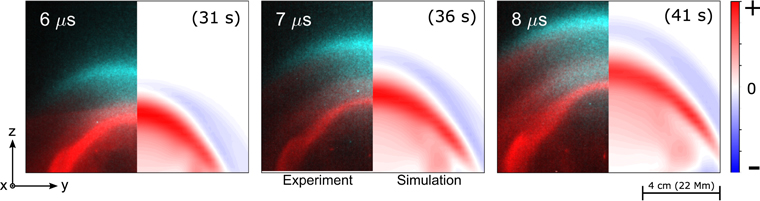
Figure 4. The left dark background halves are the image sequence of multiwavelength fast camera images of the experiment, comprising two bandpasses: visible (red) and filtered Hα (cyan). The right white background halves are the cross-sectional plots of simulated current density in horizontal direction (Jy) of the ideal 3D MHD simulation. The color bar indicates the value of Jy. In both cases, the snapshots are taken at the same time (labeled in white) after the plasma breakdown. The simulated images are taken at different times from Haw et al. (2018). The temporal and spatial quantities are scaled into the solar environment as labeled in the parentheses.
Download figure:
Standard image High-resolution imageA fast ICCD movie camera, a magnetic probe array, and Langmuir probes are used to diagnose spatial and temporal characteristics of the plasma. The optically filtered fast ICCD camera provides the series of spectroscopic images shown in the left half of Figure 4. The magnetic probe array measures the magnetic field along the z-axis from voltages induced by changing magnetic fields. Assuming that the internal evolution is much slower than the global expansion, the time evolution can be converted (Haw et al. 2018) to spatial position with  , with vz = 15 km s−1. Then
  because the spatial variation of the flux rope is mostly in the z direction (∂zBx ≫ ∂xBz). Negatively biased Langmuir probes measured ion saturation current from the plasma at a given time along the z-axis. The ion density can be inferred from ion saturation current Isat, with an isothermal assumption, i.e., ni = Isat/(0.6eAcs) with
  km s−1 and probe tip area A = 7.6 × 10⁻⁶ m2.
The solid lines in Figures 5(a) and (c) are example plots of the measured time dependence of probes at three different values of  . This data was fitted with analytic functions that are plotted as dashed lines in Figures 5(a) and (c).
  was modeled as two Gaussian peaks and
  was modeled as a piecewise function that increases linearly and decreases exponentially. The Langmuir probe data was taken from 164 shots at 24 different locations (
 ). The magnetic data were taken from 83 shots at 4 different locations (
 ). Spacetime contour plots of
  and
and  were constructed from the measurements and are shown in Figures 5(b) and (d). The positive and negative component of
  contour are scaled differently to enhance the negative component. A detailed description of the method for construction of these contour plots is given in the Appendix. These measurements, along with the lower brightness of optical line emission in between the two opposite current features from the images, imply that there is a depletion in density in the region between the two opposite currents. The Langmuir probe signals show a clear jump in density indicating a shock in ion density with thickness δ = 0.8 ± 0.3 cm and compression ratio X = 1.8 ± 0.4. Let t0 and t1 be the time in which Langmuir probe data first increase from the background level and reach the peak respectively. Then δ is deduced from the difference in the arrival times and from the speed of the feature as δ = vz(t1−t0). X is determined by the ratio of the signal at those two times,
  .
.

Figure 5. (a) and (c) show the experimental sample time-series of the magnetic and Langmuir probes (solid line) with the reconstructed fitted profiles (dashed line). (b) and (d) plot the spacetime profiles of the dashed line of  and
and  in (a) and (c). The normalized parameters for the experiment are a = 1.1 cm, vA = 0.43 km s−1, τ = a/vA = 130 μs, ρ0 = 9.1 × 10⁻⁹ kg m−3, B0 = 0.46 G, and
  = 3.3 kA m−2. These parameters can be scaled to the solar context using a = 6.25 Mm, vA = 41.7 km s−1, τ = 135 s, ρ0 = 7.0 × 10⁻¹² kg m−3, B0 = 1.2 G, and J0 = 16.7 μA m−2. The method for scaling to the solar context is given in Haw et al. (2018) and in Ryutov et al. (2000).
Download figure:
Standard image High-resolution imageThe following section describes results from a 3D ideal MHD numerical simulation of the experiment. This numerical simulation confirms that the reverse current mechanism can generate shocks and also allows a shock analysis with high spatial resolution.
4. MHD Numerical Simulation
The 3D ideal MHD simulation of the experiment was performed on the Los Alamos Turquoise cluster as part of the Los Alamos COMPutational Astrophysical Simulation Suite to reproduce the Caltech solar loop experiment (Li & Li 2003; Zhai et al. 2014; Haw et al. 2018). The simulation follows the evolution of eight parameters: mass density ρ, pressure p, velocity  , and magnetic field
  inside a numerical Cartesian box of size 32a. The initial parameters are set to emulate the experimental setup shown in Figure 3(a). The initial density consists of two conic-shape density profiles as produced by the gas nozzles at the footpoints when there is a substantial pre-filled uniform background density. The initial magnetic field is the bipolar potential field from the two solenoids behind the electrodes. The pressure is calculated from the isothermal assumption and the plasma is initially at rest. Electric current is injected into the system by adding azimuthal magnetic field corresponding to a group of circular current loops (Simpson et al. 2001; Wongwaitayakornkul et al. 2017; Haw et al. 2018) with a sinusoidal time dependence that mimics that in the experiment. Figure 4 shows the time dependence of the loop expansion as observed in the experiment (left halves of figures) and as calculated in the simulation (right halves of the figures). The simulation is in reasonable agreement with the laboratory plasma in terms of the loop's evolution and magnetic field. The full diagnostic capability of the simulation allows for more detailed analysis than possible in the experiment of the temporal and spatial dependence of the main current channel (red) and the reverse current layer (blue).
The evolution of the system can be broken down into three stages: formation, driving, and decoupling. Figure 6 shows the evolution of the apex, defined as the z coordinate of local maxima of  . Let
. Let  and
and  , where a is the minor radius of the flux rope and the nominal length for normalization and vA is the Alfvén speed. In the formation stage (
 ), a current flowing in the positive y direction is injected into the system. The curved current channel expands in major radius due to its hoop force and compresses in the positive z direction, forming a flattened current channel flowing mainly in the positive y direction. Later in the driving stage (
 ), a reverse current layer is formed above the original expanding current channel; this reverse current is formed to satisfy the magnetic flux conservation condition in the stationary conducting background plasma above the current channel. The increased azimuthal magnetic field in between the main and reverse currents pushes the reverse current layer out radially and leaves behind a region of depleted density (region between the red and blue regions in Figure 3(a) and in Figure 4). The plasma boundary, or contact front (bottom of the blue region in Figure 4), acts as a magnetic piston, compressing the swept-out plasma. With sufficiently strong current, the piston expands faster than the magnetosonic speed in the plasma. As a result, a shock is formed ahead of the piston and all the mass swept up by the shock is compressed into a thin layer immediately behind the shock. The current layer and the shock are indistinguishable at this stage. The thin current layer is repelled by the core current and quickly reaches the equilibrium standoff distance as prescribed by Equation (9). The full dynamics of the induced current sheet are governed by the force balance of fe and fc, described in Section 2.2. At
  , the current injection stops, causing the driver and the contact front to decelerate. With the condition described in Section 2.1, the contact front and the shock separate. The shock remains in motion, while the contact front decelerates with the driver. Thus, for
  the shock is decoupled from the piston and propagates freely.
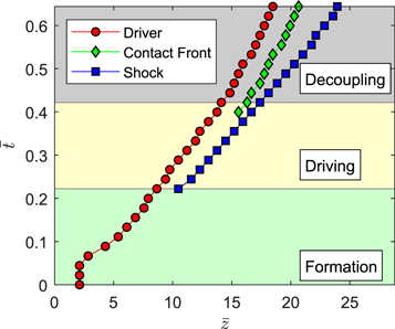
Figure 6. Evolution of apex locations of the simulation during the three stages.
Download figure:
Standard image High-resolution imageThe analytic theory presented in Section 2 used the cylindrical coordinate system shown in Figure 2. In this section we present a result of a numerical simulation where Cartesian coordinates are used instead. The correspondence follows  . Since the apex moves in the z direction, it is convenient to plot the parameters along the z-axis. Figure 7(a) plots contours of
  as a function of
  and
and  . Recall that
  is the horizontal component of the current at the apex as shown in Figure 3(a). Figure 7(a) shows the main current channel in red and the reverse current in blue slightly to the right of the red. The experimental
  contour in Figure 3(b) shows a larger decay of amplitude in
  compared to its simulated counterpart in Figure 7(a). This is expected due to a higher resistivity in the experiment. The slope,
  , of the reverse current layer in Figure 7(a) implies a propagation speed
  = 25, which exceeds the local fast magnetosonic speed
  = 10 of the unshocked plasma.

Figure 7. Time evolution of four quantities from the MHD simulation in z along the apex. The plots consist of (a) current density, (b) temperature, (c) mass density, and (d) flow speed. For coronal environment, the normalization quantities are a = 6.25 Mm  , vA = 41.7 km s−1, τ = a/vA = 135 s, ρ0 = 7.0 × 10⁻¹² kg m−3, B0 = 1.2 G,
  = 16.7 μA m−2, and
  K (mH = 1 u).
Download figure:
Standard image High-resolution imageThe transition is therefore a fast-mode shock and should obey the RH relations given in Section 2.1. Figure 7(b) plots the temperature  , showing that the loop becomes cooler as its size increases. This is expected from the adiabatic equation of state. The main current channel, however, remains the hottest part even after the shock forms. The density
  , in Figure 7(c), shows that the density amplification is largest at the location of the shock front. Behind the shock, the density depletes to a value lower than the background (black region). Contrary to the experiment (Figure 3(c)), the simulated density contour (Figure 7(c)) appears to contain a single peak at most times. A two-peak profile can only be observed when the shock is initially formed, i.e.,
  . The density peak of the main current decays abruptly, while the density peak of the shock remains more or less constant. As the system expands, the volume increases. However, only the shock acquires the additional material from the background plasma. In the experiment, the plasma behind the electrode most likely supplies material to sustain the density of the main current loop. Lastly, the velocity plot, shown in Figure 7(d), exhibits the initially fast expanding loop due to the strong flow of material behind the loop. At
  , the plasma behind the loop experiences a large magnetic force in the positive z direction from the current injection indicated by its large vz. For
  , the shock front and its plasma flow reach constant terminal speeds.
Figure 8 displays the set of quantities, in the frame moving with the shock of speed  , on the shock boundaries at time
  from the simulation; this time it is denoted as "shock" in Figure 7.
  is the plasma density,
  is the gas pressure,
  is the velocity in z direction, and
  is the tangential magnetic field in the xy-plane. The flow speed in the shock frame is defined as
  . This relation is obtained by (i) moving to a shock frame
  and (ii) flipping the sign
  to have
  be positive in the
  direction. The subscripts u and d represent the upstream and downstream value of the parameters, which are taken from the boundary of the shocks denoted by the vertical dashed lines in Figure 8. Given that the fast magnetosonic speed is always greater than the Alfvén speed
  , the background colors specify three regions in velocity phase space based on
  : (i)
: (i)  , (ii)
  , and (iii)
  . The shock takes the plasma flow from region (i) to (ii), which is the characteristic of the fast magnetosonic type.

Figure 8. Transition of four variables in the MHD simulation: flow velocity in the shock frame  , mass density
  , pressure
  , and tangential magnetic field
  across the shock. The
  range and time for this plot are shown as the magenta line in Figure 7. The background colors represent the three regions in velocity phase space: (i)
  , (ii)
  , and (iii)
  . The two vertical dashed lines indicate the boundaries of the shock. Each parameter is normalized to their upstream value. The expected compression ratios are labeled Y, X, and X−1 on the downstream boundary.
  is the location of shock center and
  is the shock thickness.
Download figure:
Standard image High-resolution imageGiven the characteristic of the background plasma  and β, we may now calculate the expected compression ratios X and Y using Equations (5) and (6). For the simulation at the time
  , the compression ratios can be determined from the upstream parameters
  ,
,  ,
,  ,
,  , which gives
  , β = 136. Using these values in Equations (5) and (6) gives X = 2.1 and Y = 3.8, as indicated with diamond markers in Figure 8. The simulated compression ratios are
  ,
,  ,
,  , and
, and  , where upstream and downstream values are measured at the locations of the vertical dashed lines. These compression ratios are also consistent with the analytic expression in Section 2.2. The simulated compression ratios match well with the analytic expression for
  and
and  , indicating that the perturbation front is a fast magnetosonic shock. For
  , β = 136, and γ = 5/3, the magnetosonic mach number
  . The normalized entropy,
  , also increases across the shock (
 ).
).
The simulation shows that a flux rope erupted from the injection of the electrical current induces a layer of reverse current that acts as a magnetic piston. Impulsive expansion of the piston produces a fast-mode shock that is also a current layer due to the compression of the background magnetic field. The dynamics of the piston is described in Section 2.2 and is compared to the simulation in Haw et al. (2018). In the driving phase, the shock and piston are attached. Thus, the shock evolution is governed by the movement of the driver, displaying the characteristic of a pseudo-wave. In the decoupling stage, the shock detaches from the piston because the piston decelerates to a speed below the local fast magnetosonic wave speed. The piston and shock separate and so the shock escapes the driving influence of the piston. The shock is then self-propagating, representing the wave behavior. The presence of both the wave and pseudo-wave behavior of the simulated shock supports a hybrid theory of CME-driven EUV wave.
5. Discussion
Despite the variety of different models to explain EUV waves, the physical manifestation of all proposed models is a propagating, compressive current layer. This current layer is caused by compression of the background magnetic field, but in previous models this current was not identified as being in the reverse direction with respect to the current in the erupting flux rope. Fast-mode pulses/shocks are, by definition, compressive current layers. The current layer model in Delannée et al. (2008) was previously characterized purely in terms of the electric current; however, it is also cospatial with a compressive density pulse. The wake model in Chen et al. (2002) identifies the EUV wave as a compressive front but does not take into account that a compressional front must necessarily contain electric current. Finally, the successive magnetic reconnection model in Attrill et al. (2007) creates an expanding density enhancement with electric current. This is not implying that all the models are equivalent, but instead highlights the overlap of the differences. In some cases, such as the current layer (Delannée et al. 2008) and wake models (Chen et al. 2002), it is not clear if there is a physical distinction between these two models (Long et al. 2017). Table 1 in Long et al. (2017) presented predictions of pulse physical properties from six previous theories and Table 2 of Long et al. (2017) showed how these predictions compare to observations. Table 1 of the present paper shows the predictions given by the model presented in this paper for the properties listed in Long et al. (2017).  and
and  represent the lateral velocity and acceleration of the erupting CME. ACME represents the area bounded by the CME bubble. These predictions are similar to the previous fast-mode wave/shock and current shell theory, which are in good agreement with observations. The physical manifestation of the pulse would then be dictated by whether the time of observation is in the driving or decoupling phase of the event.
Table 1. Prediction from This Model for the Properties Listed in Long et al. (2017)
| Pulse Properties | This Hybrid Model | ||
|---|---|---|---|
| Driving Phase | Decoupling Phase | ||
| Small amp. | Large amp. | ||
| Linear Wave | Wave/Shock | ||
| Phase velocity [v] |

|
vms | >vms |

|
>
|
||
| Acceleration [a] |

|
0 | <0 |
| Broadening | f( ) ) |
≈0 | >0 |
| ΔB | >0 | >0 | >0 |
| ΔT | Adia.+QJoule | Adia. | Adia.+Q |
| Δne | Compression | Compression | Compression |
| Height | f(CME bubble) | f(B, ne) | f(B, ne) |
| Area bounded | ACME | >ACME | >ACME |
| Rotation | Possible | Possible | Possible |
| Reflection | No | Yes | Yes |
| Refraction | No | Yes | Yes |
| Transmission | No | Yes | Yes |
| Stationary fronts | Yes | Yes | Yes |
| Cospatial Type II | No | No | Possible |
| Moreton wave | No | No | Possible |
Download table as: ASCIITypeset image
The hybrid model proposed here is consistent with existing observations. The main observation supporting the fast-mode shock model is the strong correlation between the type II radio burst and the EUV waves (Klassen et al. 2000; Biesecker et al. 2002; Vršnak & Cliver 2008). Assuming the density profile of the corona, one could deduce the speed of the emitter from the radio signals, which turns out to be faster than the coronal Alfvénic speed, suggesting that the emitter is a coronal shock front. In addition, CMEs are strongly correlated with the observation of EUV waves (Biesecker et al. 2002; Warmuth et al. 2005; Veronig et al. 2008). Figure 9 shows a system of flux rope and shock for both an AIA observation on 2010 June 13 and our laboratory experiment in reverse grayscale (i.e., black is the maximum value and white is the minimum value). We have shown that an erupting flux rope can generate a fast magnetosonic shock. The fast magnetosonic shock generated by an erupting CME should then be able to produce the type II radio burst.

Figure 9. Comparison of (left) the low coronal EUV (193 Å) shock wave observed with AIA/SDO on 2010 June 13 (courtesy of NASA/SDO and the AIA, EVE, and HMI science teams; it is the same image as used in Ma et al. 2011) and (right) visible emission from the Caltech experiment in reverse grayscale.
Download figure:
Standard image High-resolution imagePreviously measured compression ratios of the observed global EUV wave, deduced from the intensity ratios of line emission, are 1.05–1.30 (Muhr et al. 2011; Zhukov 2011; Long et al. 2015). In the numerical MHD simulation shown in Figures 6–8, we obtain the compression ratio of X = 1.9, which is different from the observed values due to the different  and β of each event; Equation (7) shows the relation between X,
  , and β. For example, substituting
  (note that
  ) and β = 0.1 into Equation (7) gives X = 1.27, as presented for the 2007 May 19 event in Muhr et al. (2011). While a uniform β = 0.1 is commonly used at z ∼ 70–200 Mm (0.1 R⊙–0.2 R⊙ Ma et al. 2011; Long et al. 2015) above the solar surface as suggested by Gary (2001), a more recent simulation (Bourdin 2017) proposed that a varying β = 20–200 is more suitable in that region. This range of β is used in our simulation. If we were to use
  and β = 136, the corresponding X according to Equation (7) would also be X = 1.27. Figure 10 shows the contour of compression ratio X in
  -space. X = 1.27 is drawn with a solid line. The two points (
 ) and (
 ) both correspond to X = 1.27 and are plotted with green and blue markers, respectively. For β ≫ 10, X is no longer sensitive to β and the shock approaches the hydrodynamic limit. While β and vms are the properties of the background plasma, the expanding speed of the structure depends on the internal current of the CME's core, as discussed in Section 2.2. Consequently, the observation of the global EUV waves and their measured compression ratios could give us insight into the eruption mechanism of the CME.

Figure 10. Contour of the compression ratio  as determined by Equation (7). The compression ratio of the 2007 May 19th event in Muhr et al. (2011) X = 1.27 is plotted as a solid line. The two points corresponding to β = 0.1 and 136 along X = 1.27 are plotted with green and blue markers. The value used in the simulation of this work is plotted with a red marker.
Download figure:
Standard image High-resolution imageThe reverse current piston can produce both waves and shocks, depending on the driving and observing timescale. When the piston moves at a speed below the fast magnetosonic speed of the background plasma (vpiston < vms), the piston drives a simple wave that can eventually steepen into a shock. When vpiston > vms, a shock forms due to the piston effect. In this case, the shock evolves in two stages: (i) attached to the driver and then (ii) decoupled from the driver. Depending on the time of the observation, the compressional front can behave as a wave or a pseudo-wave. The shock exhibits pseudo-wave behavior and wave behavior in stages (i) and (ii), respectively. The analytic model can be used to predict the condition, time, and height in which the two stages occur. This can explain why EUV waves are sometime slower than the expected coronal fast-mode speed (Wills-Davey et al. 2007). Several observations had reported detecting two-component bright fronts with either sharp (Liu et al. 2010) or diffuse (Cohen et al. 2009; Cheng et al. 2012) outer structure, which could respectively correspond to shock (sharp) and wave (diffuse) perturbation driven by a bright sharp piston current layer. The magnetic piston decelerates late in the simulation and eventually reaches a stationary equilibrium where the internal magnetic pressure balances the external background pressure. This could be an explanation for the observed deceleration (Warmuth et al. 2004; Long et al. 2008; Veronig et al. 2008) and stationary brightenings (Ofman & Thompson 2002; Terradas & Ofman 2004). The existing observations, supporting wave/pseudo-wave bimodality (Harra & Sterling 2003; Patsourakos & Vourlidas 2009; Chen & Wu 2011; Ma et al. 2011), show the transition from pseudo-wave to wave as illustrated in Figure 6. Future observations of high-cadence detailed kinematics of the decoupling process would provide a rigorous test for this hybrid model.
In summary, a single description of EUV waves as compressional MHD perturbations reconciles the important features of previous models and is supported by a laboratory experiment and a numerical simulation. A magnetically induced reverse current layer produced by an erupting flux rope creates a single coherent pulse that can be observed as a wave, pseudo-wave, and shock, depending on the plasma parameters and driving/observing timescale. By applying this interpretation of the coronal pulse generating mechanism, EUV wave observations could be used to diagnose the internal structure of CMEs.
This work was supported by NSF/DOE Partnership in Plasma Science and Engineering under award DE-FG02-04ER54755 and AFOSR under award FA9550-11-1-0184. H.L. acknowledges support from the DoE/OFES and LANL/LDRD programs.
Appendix: Experimental Contour Reconstruction
The following steps are used to create the spacetime contour plots shown in Figures 5(b) and (d):
- 1.A single point measurement at location
 and gives experimental time-series and , respectively.
 - 2.
- 3.For a given pair of, the comparison between the experimental and constructed profile gives fitting parameters for this particular pair of :
- 4.The pair is varied through its domain to determine the dependency of each parameter. The Cj's are determined by best fit to the measured data. The models are chosen as follows:
- (a)J± is modeled as an exponential decay, i.e.,. The current is assumed to decay exponentially due to the magnetic diffusion. The extrapolation of to small is consistent with the expected value, i.e., Jy,expected = 1 kA/(π .
- (b)ρi and ti for i = 0, 1, 2, 3 are fitted as second degree polynomials with respect to, for example, . The Langmuir probe data covers most of the range of . Therefore, we choose the simplest smooth curve function to fit these parameters. t± lie well with the best fit of t1 and t3 within their domain, so we set and .
- (c)τ± and λ are chosen to be constants, i.e., and . From observations, the widths do not change with as much as the other parameters. Thus, for simplicity, the widths are assumed to be constant for all .
- 5.Figures 5(b) and (d) are obtained by plotting contours in the spacetime domain using the constructed functions:


