


Abstract
We study the mass of quasar-hosting dark matter halos at z ∼ 6 and further constrain the fraction of dark matter halos hosting active quasars fon and the quasar opening angle imax using observations of C ii lines in the literature. We make assumptions that (1) on average more massive halos host quasars with higher peak brightness, (2) cold gas in galaxies has rotational velocity Vcirc = αVmax, where Vmax is the maximum circular velocity of dark matter particles obtained from DM-only simulation and α ∼ 1 is a free parameter, (3) a fraction fon of the halos host active quasars with a certain opening angle imax, and that (4) quasars point randomly on the sky. We find that for a choice of specific α ≳ 1, the most likely solution has fon < 0.01, corresponding to a small duty cycle of quasar activity. We also apply a bounded flat prior on α and marginalize over it, and we find the most likely fon shift to 1 as the upper-boundary of α decreases below 1. Overall, our constraints are highly sensitive to α and hence inconclusive. Stronger constraints on fon can be made if we better understand the dynamics of cold gas in these galaxies.
Export citation and abstract BibTeX RIS
1. Introduction
Despite the mounting evidence that the Epoch of Reionization (EoR) ends at z ∼ 6, many details on how the universe gets reionized remain poorly understood. One of the outstanding problems in EoR research is the contribution of quasars to the total ionization history. Presently, there is no conclusive answer to this problem: many studies suggest that quasars may not play a major role in driving reionization on large scales (e.g., Onoue et al. 2017), though others indicate that there is still possibility that quasars drive cosmic reionization (Madau & Haardt 2015). However, it is well-recognized that quasars dominate the reionization process in their local environments (Lidz et al. 2007; Kakiichi et al. 2017). Their powerful ionizing radiation creates proximity zones where H and He are overionized relative to the general universe. In the proximity zones, galaxy formation may be delayed (Kitayama et al. 2000). How many galaxies are impacted by quasars is closely related to quasar lifetime, opening angles, and more importantly how over dense the quasar environment is, which unfortunately are all very uncertain.
Due to the increased halo clustering near higher-mass halos, the mass of a quasar-hosting halo determines the number of nearby galaxies that may be impacted by the quasar. Therefore, to study reionization history in quasar surroundings, it is important to understand how massive their host halos are.
Masses of quasar-hosting halos can be estimated in many different ways (Martini 2004). In the local universe, one can connect the black hole mass to the host halo mass by using the tight M–σ relation (Ferrarese & Merritt 2000; Gebhardt et al. 2000; Kormendy & Ho 2013; Pacucci et al. 2018) and the correlation between the circular velocity and the bulge velocity dispersion (Ferrarese 2002). At higher redshifts, one can measure the relation between the quasar luminosity and the clustering length, which in turn can be translated into the mass of quasar-hosting halos (Haiman & Hui 2001; Martini & Weinberg 2001). For example, Shen et al. (2007) used SDSS data and found a minimum halo mass (4–6) × 1012 M⊙ at 3.5 < z < 5.3 for their sample.
However, at z ∼ 6, studies of quasar host halos are rare. Although recent surveys have found ≳100 quasars at z ∼ 6 (Fan et al. 2006; Bañados et al. 2016), this number is still too small for a reliable clustering measurement. Fortunately, recently ALMA opened a new window into such studies. Thanks to its exceptionally high spatial and spectroscopic resolution, it is possible to map many z ∼ 6 quasar host galaxies in millimeter molecular lines and measure their emission line profiles. Emission lines from cold gas offer dynamical information, which is crucial in determining the halo mass.
Measuring quasar halo masses has a further fascinating application of constraining quasar duty cycles. If we assume all dark matter (DM) halos host a quasar, then small quasar-hosting halo mass indicates a large number of quasars are not active, suggesting a small quasar duty cycle. Using clustering method, Shen et al. (2007), Shankar et al. (2010) found increasing duty cycle from fduty ∼ 0.01 at z = 1.45 to 0.03–0.6 at 3.5 < z < 5.3.
In this paper, we use updated observational data from the literature (mainly ALMA observations) to estimate quasar-hosting DM halo mass. We use a simple model to put constraints on the fraction of DM halos that host a visible quasar fqso and the quasar opening angle imax. We describe our methods in Section 2 and show the results of constraining fqso and imax in Section 3. The discussion and conclusions are presented in Sections 4 and 5.
2. Methodology
Our main goal is to study the relation between the quasar luminosities and the mass of DM halos they reside in at z ∼ 6, and further constrain the quasar duty cycle and the opening angle. For this purpose, we make several assumptions described below, and use C ii line profiles of 44 known z ∼ 6 quasars in Decarli et al. (2018) to estimate the halo mass.
2.1. Assumptions
We list our assumptions hereafter and review them in greater detail in the discussion:
- 1.Every DM halo hosts an SMBH, and more massive halos host brighter quasars.
- 2.Cold gas in quasar-hosting galaxies is rotationally supported with a flat rotation curve of Vcirc. Vcirc is linked with the maximum of circular velocity of DM particles Vmax by Vcirc = αVmax, where α ∼ 1.
- 3.Among all DM halos, a fraction of them (fon) host active quasars, and quasars have the same opening angle imax, corresponding to a solid angle of 4π (1 − cos(imax)).
- 4.The distribution of quasar orientation is random with the sole constraint that the inclination angle i is smaller than the quasar opening angle imax (otherwise the quasar cannot be detected optically).
Our key assumption is that brighter quasars reside in more massive halos (Haiman & Hui 2001; Martini & Weinberg 2001; Shen et al. 2007; Shankar et al. 2010; La Plante & Trac 2016). This is probable because large halos at z ∼ 6 must experience fast accretion, which may also indicate fast quasar fueling process (Martini & Weinberg 2001). Observations also support this assumption and indicate a narrow scatter (Shankar et al. 2010). We adopt an abundance-matching ansatz:

where n(>L) is the number density of quasars with luminosity larger than L, and n(>Mh) is the number density of DM halos with mass larger than Mh. The parameter fqso is the fraction of halos that host visible quasars. Due to the fact that quasars have limited lifetimes and are obscured when inclination angles are larger than imax, fqso should be:

By matching the number densities of quasars with the number density of DM halos, we can obtain the relationship between quasar luminosity and the underlying halo DM mass:

We use ϕ(L) from Onoue et al. (2017). We note that although the faint end of the quasar luminosity function is still uncertain, this does not affect our results because the observed quasars mainly populate the bright end.
2.2. Halo Mass Function
There exist a number of analytical fits for halo mass functions. Unfortunately, analytical fitting formulas at z ∼ 6 are of considerable differences (Lukić et al. 2007; Tinker et al. 2008; Murray et al. 2013; Reed et al. 2013; Watson et al. 2013). For this reason, we use the halo catalog of our existing CROC simulations (Gnedin 2014) to determine what analytical halo mass function to use. We find that the Tinker08 (Tinker et al. 2008) halo mass function agrees exceptionally well with numerical simulations of z ∼ 6 universe in the mass range of 109–1012 M⊙ (the massive halo regime), both in terms of amplitude and shape.
Using the Tinker08 halo mass function and the quasar luminosity function from Onoue et al. (2017), we obtain the function of quasar luminosity and halo mass with different parameter fqso, shown in Figure 1. A smaller value of fqso results in smaller halo mass because more halos are required to match the observed quasar number density at certain M1450.
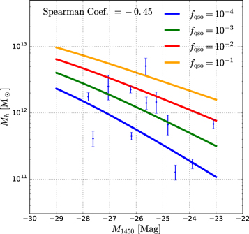
Figure 1. Abundance-matching results for different values of the parameter fqso. A smaller value of fqso results in smaller halo mass. Blue dots are quasars in the literature with C ii maps available and galactic disks marginally resolved. Error bars only account for the uncertainties in FWHM measurements. The data have a Spearman coefficient of −0.45, showing a weak anti-correlation.
Download figure:
Standard image High-resolution image2.3. Estimating the Virial Mass
To obtain the virial mass from observations requires several assumptions. Observations typically only provide some velocity information from spectra. We need to find a relation between mass and spectroscopic observables.
In DM-only simulations, the maximum of circular velocity Vmax is tightly correlated with the virial mass of DM halos. Using the publicly available 250 Mpc/h Bolshoi halo catalog (Klypin et al. 2011; Behroozi et al. 2013a, 2013b), we fit the z ∼ 6 halos and found a best-fit power-law relation of

with a scatter of 4% for halos above 1011 M⊙.
We denote rmax as the radius at which Vmax is reached. For a 1 × 10¹² M⊙ halo at z ∼ 6, the virial radius is ∼70 pkpc, and rmax is ∼30% of the virial radius.
In order to connect gas motions to Vmax, we assume that gas has a flat circular velocity profile with Vcirc = αVmax inside rmax. We treat α as one of the key parameters and discuss it further in Section 3.
2.4. Compilation of Observation Data
Singly ionized carbon C ii line at 158 μm traces cold gas, which is thought to be bound and rotationally supported within the dark matter halo (Wang et al. 2013). For z ∼ 6 galaxies, this line redshifts to mm-wavelength, which can be observed by radio interferometers like ALMA. We thus use C ii spectra to constrain halo masses.
We use the list of 44 z ∼ 6 quasars from Tables 2 and 4 in Decarli et al. (2018), particularly the FWHM of C ii emitted from their host galaxies.
Viewing angle affects the line width. In practice, inclination angles (the angles measured between the line of sight and the normal vector of the disk) are usually estimated by the semiminor to semimajor axis ratio i = arccos(b/a). If we use the inclination angle measured this way, and using (Wang et al. 2013; Willott et al. 2015; Decarli et al. 2018)

we can estimate the halo mass. In the literature, there are 12 quasars with marginally resolved disks (Wang et al. 2013; Stefan et al. 2015; Willott et al. 2015, 2013, 2017; Venemans et al. 2016, 2017; Decarli et al. 2018). We calculate their halo masses assuming α = 1 and overlay them as blue points on Figure 1, with error bars including only the observational errors on the FWHM. There is a weak anti-correlation between M1450 and Mh (Spearman's rank correlation coefficient = −0.45), and the data marginally exclude fqso = 0.1.
However, limited by the resolution of current observations, the lengths of galaxy axes can at best be marginally measured at z ∼ 6: most of the 12 galaxies above have spatial sizes only less than two beam sizes of the telescope. The rest of quasar-hosting galaxies in the sample (32 out of 44) are not resolved at all. Considering the large uncertainty in the inclination angle measurements, we use another method to place constraints on fqso using all 44 galaxies in the sample. We assume that the orientation of quasar beams is random on the sky, with a maximum inclination angle imax. Using a threshold, imax is motivated by the limited opening angle of quasar, usually around 45° (Zhuang et al. 2018).
The cumulative probability distribution of the inclination angle for random orientation is the area of a sphere where the azimuthal angle is smaller than i, divided by the total area of the sphere with the maximum azimuthal angle imax:
For a fixed parameter fqso, for each observed quasar we can calculate the inclination angle i such that the quasar lies on the relation set by the abundance-matching ansatz (3). To constrain fqso, we use the Kolmogorov–Smirnov (K–S) test to compare the distribution of i obtained to the assumed random distribution with maximum inclination angle imax.
We show examples of this distribution in Figure 2 for two parameters combinations (fqso, imax) = (0 004, 63°) and (01, 40°). In the left panel, the calculated cumulative distribution function (CDF) of i (blue solid line) lies close to the model distribution (red dashed line), with a p-value of 0.4, suggesting that the assumption that quasars are randomly oriented is highly probable. In the right panel, the calculated CDF lies systematically below the red model CDF, with a small p-value of 0.018. This implies that either imax is underestimated or fqso is overestimated.

Figure 2. Comparison of the derived and expected cumulative inclination angle distributions for two representative sets of values (fqso, imax) = (0004, 63°) (the most likely values) and (01, 40°), respectively.
Download figure:
Standard image High-resolution image3. Constraints on the Visible Quasar Fraction
In Figure 3, we show the p-values for different combinations of fqso and imax for three choices of α ≡ Vcirc/Vmax. The value of α = 1 can be considered as characteristic, but it can be smaller if the C ii-emitting gas occupies only the very inner part of a halo and does not dominate the gravity within rmax. It can also be larger than 1, as low-redshift large-spiral galaxies often have α = 1.2–1.4 (Navarro et al. 1997). We note that there is no acceptable solution for α < 0.6.
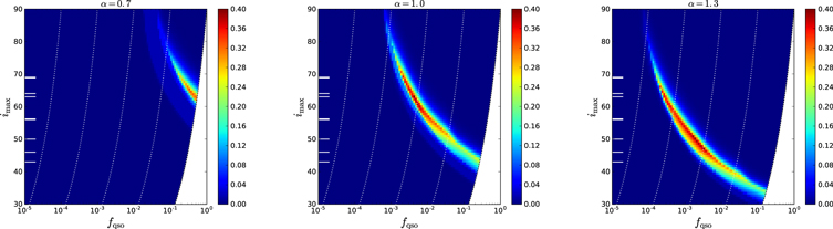
Figure 3. P-values of K–S tests for different combinations of (fqso, imax) for three particular choices of α ≡ Vcirc/Vmax = 0.7, 1.0, and 1.3 (left to right). Note that fqso and imax are strongly correlated, because a larger value of fqso can be counteracted by a smaller quasar opening angle. Dotted lines show different values of fon (2): from left to right the values are fon = 10−4, 10−3, 10−2, 10−1, respectively. The lower right region is prohibited due to the constraint fon ≤ 1 (Equation (2)). Solid white horizontal lines mark observed inclination angles from resolved ALMA galaxies.
Download figure:
Standard image High-resolution imageAs can be seen from the figure, fqso and imax are strongly correlated, because larger fqso corresponds to larger halo masses for fixed M1450; in order to obtain the observed FWHM, the assumed inclination angles must decrease, and in order to match the observed i distribution, imax must decrease as well. For α ≥ 1, the maximum p-value occurs at small values of fqso, suggesting that quasars at z ∼ 6 reside in fairly low-mass halos (see Figure 1).
The short white lines on the left side of Figure 3 are values of the inclination angle iimg estimated from the C ii maps of marginally resolved quasar host galaxies (thicker lines represent two galaxies that have the same measured inclination angle). The maximum opening angle imax should lie close to the few largest iimg.
The most probable values of fqso and imax depend strongly on the choice of α. One possible way to remove that dependence and to account for the lack of knowledge in the proper value of α is to "marginalize" over it,
where wα is the prior on α. Notice that it is namely pKS that should be integrated, as it is a measure of the probability density and a direct analog of a likelihood in this case. In that case, however, we need to adopt an upper limit to the integral, αmax.
The marginalized distributions of p-values are shown in Figure 4 for the three choices of αmax. In this case, in addition to a low fon solution, a solution with fon also appears for αmax = 1, which becomes the sole solution at lower αmax. For αmax = 1 (middle panel), the most probable (fqso, imax) = (004, 55°), corresponding to fon = 0.08. However, the region around (fqso, imax) = (03, 48°), corresponding to fon = 1, also has a high probability. For the upper-boundary of prior αmax = 0.7 < 1 (left panel), the only possible solution is fon = 1, while for αmax = 1.3 > 1 (right panel), the most likely fon < 0.01.
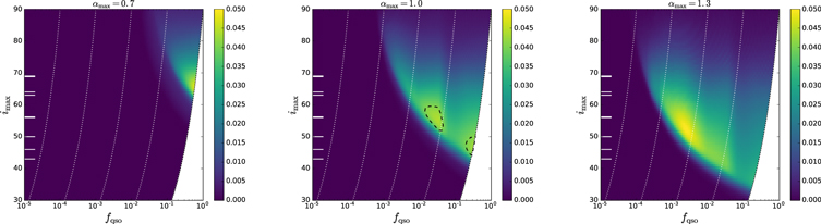
Figure 4. Same as Figure 3, but now with p-values marginalized over α. In the middle panel, the two black dashed contours (pKS,marg = 0.04) mark the regions around the global (left) and a local (right) maximum.
Download figure:
Standard image High-resolution image4. Discussion
4.1. Review of the Assumptions
In creating Figure 1, we have made several assumptions. Here we discuss assumptions (3) and (4) and check how the results change when we vary these assumptions.
4.1.1. Abundance-matching Ansatz
The assumption that more massive halos host brighter quasars has a physical background and has been used in many studies (Haiman & Hui 2001; Martini & Weinberg 2001; Shen et al. 2007; Shankar et al. 2010; La Plante & Trac 2016). However, it is important to note that there are some cases for which this assumption could fail.
Indeed, the assumption is generally based on an idealized picture that quasars exist in one of only two states: "on" and "off". In the "on" state, more massive halos accrete faster and all SMBHs have a similar radiative efficiency; hence, a faster fueling SMBH is brighter. In reality, this may not always be the case.
First, mass accreted by the host halo is not necessarily proportional to the mass fed into the SMBH, due to various feedback processes. As fueling process fluctuates with radiative feedback, luminosity may also change quasi-periodically (Pacucci & Ferrara 2015). In the abundance-matching ansatz the halo mass—quasar luminosity relation is established only on average, so such fluctuations from individual quasars average out, but whether they average out sufficiently to maintain the approximately monotonic relation between the halo mass and the peak quasar luminosity remains to be seen.
Moreover, for some radiatively inefficient models (Shakura & Sunyaev 1976; Inayoshi et al. 2016; Begelman & Volonteri 2017), the quasar luminosity only mildly depends on the accretion rate and can easily violate the abundance-matching ansatz. Such inefficiently accreting quasars are expected to be faint and hence are treated as being in the "off" state in our model. However, some of them may still be bright enough to be confused with lower-mass black holes in the "on" state. Our sample of observed quasars spans only a factor of ∼10 in quasar luminosity (with a few fainter quasars and one very bright one), so significant contamination from inefficiently accreting quasars appears to be unlikely, but we cannot presently rule it out completely without further study.
Keeping all these caveats in mind, and given that there is observational evidence for brighter quasars clustering stronger (Shankar et al. 2010), we consider the assumption that quasars with higher peak luminosity (i.e., luminosity in the "on" state) reside in more massive halos is very reasonable.
4.1.2. Random versus Ordered Motions
The assumption that cold gas motion is rotationally supported is motivated by the clear velocity gradients found in three galaxies in Wang et al. (2013). Simulations of high-redshift galaxies also clearly show that gas forms thin disks (Rosdahl et al. 2018).
However, if we assume otherwise—that the C ii-emitting gas has completely random motions—then the line profile is independent of the viewing angle. Hence, the halo mass can be estimated by

We plot the halo masses calculated in this way as red points in Figure 5, with the halo mass uncertainties estimated from the FWHM measurement errors only. The observational points scatter widely in the y direction and do not show any significant trend. Indeed, the Spearman's rank correlation coefficient is −0.24, and thus cannot be fit with any parameter fqso. Also, most points lie below the line of fqso = 10−4, which is too small a value to be considered theoretically possible (Martini 2004). This implies that the random gas motion assumption is not valid.

Figure 5. Same as Figure 1, but with red dots showing quasar masses calculated under the assumption of random gas motion. Error bars are purely from uncertainty in the FWHM measurements. The data have a Spearman coefficient of −0.24, showing no correlation.
Download figure:
Standard image High-resolution image4.1.3. Random Orientation Model of Quasar
Random orientation of a quasar should be a good assumption, since there is no reason to expect quasar axes to be aligned. However, since different quasars may have different opening angles, the CDF may differ from Equation (6) near imax. A more complicated model may use some tapering functions near imax, but the existing data could not constrain it well.
Tapering near imax may change the K–S test results and impact the most likely values of fqso and imax. To examine the impact of such a modification to our approach, we test a simple modified CDF model with a linear function between (0.9imax, CDF(0.9imax)) and (90°, 1) (see Figure 6). Using this model, the most likely fqso and imax changed from (0.004, 63) to (0.002, 68) and fon is still <1%.

Figure 6. Similar to Figure 2, but using a modified model (red dashed line) with a linear function between (0.9imax, CDF(0.9imax)) and (90°, 1) for the CDF of quasar viewing angles. The figure shows the most likely combination of imax and fqso (p-value = 0.459); fqso changed to a smaller value compared to the "standard" random distribution model from Figure 2.
Download figure:
Standard image High-resolution image
5. Conclusions
Our attempt to constraint the high-redshift quasar lifetimes using the observed values for the velocities of C ii-emitting gas is not entirely conclusive. We find that the final answer depends extremely strongly on the assumption of how the C ii-emitting gas populates galactic halos. For the choice of α ≡ Vcirc/Vmax = 1, our results show a very small value of fon = 0.007, which decreases further if α is allowed to exceed unity. When we marginalize over α with a flat prior, a second solution appears with fon = 1; that solution, however, disappears if the adopted range for allowed α extends to values above 1. If each DM halo does indeed host a quasar and the fraction of active quasars at z ∼ 6 reflects the time fraction spent in the quasar phase for each DM halo fon = fduty, the low fon value implies a surprisingly small duty cycle at z ∼ 6. Considering that the mass of a supermassive black hole at z ∼ 6 can be larger than 109 M⊙ (Wu et al. 2015), the small duty cycle implies that the accretion e-folding time must be very small. This further implies that the large fraction of SMBHs accrete mass with no significant emission. Another explanation for this small fon is that only a small fraction fBH of halos host an SMBH: fon = fBH .
.
The small value of fon ≲ 0.01 is still consistent with the value of quasar lifetime of 107 yr that has been found in studies using the transverse proximity effect (Borisova et al. 2016). Using quasar clustering, Shen et al. (2007) and White et al. (2008) found a much larger duty cycle approaching unity. All of these studies, unfortunately, are subject to significant uncertainties. For example, the clustering method suffers from large measurement uncertainties, while our constraint on fon is strongly sensitive to the assumption of how the C ii-emitting gas populates its host halos.
The second solution with fon = 1 may be more "appealing", as it is consistent with theoretical expectations that high-redshift quasars must maintain high accretion rates to reach the observed values for their central SMBH by z ∼ 6, and is in better agreement with the clustering value. However, our main conclusion is that, at present, the data do not select one solution over the other. It is also possible that both solutions are realized in nature as two separate modes of quasar activity.
A significant improvement on this study is possible if one can constrain the distribution of α, for example, from high-resolution numerical simulations. A purely observational improvement is possible if additional ALMA-detected galaxies become resolved with reliable determinations of their inclination angles.
Fermilab is operated by Fermi Research Alliance, LLC, under Contract No. DE-AC02-07CH11359 with the United States Department of Energy. This work was partly supported by a NASA ATP grant NNX17AK65G. Some of the simulations and analyses used in this paper have been carried out using the Midway cluster at the University of Chicago Research Computing Center, which we acknowledge for support. This research also used resources of the Argonne Leadership Computing Facility, which is a DOE Office of Science User Facility supported under Contract DE-AC02-06CH11357. An award of computer time was provided by the Innovative and Novel Computational Impact on Theory and Experiment (INCITE) program. This research is also part of the Blue Waters sustained-petascale computing project, which is supported by the National Science Foundation (awards OCI-0725070 and ACI-1238993) and the state of Illinois. Blue Waters is a joint effort of the University of Illinois at Urbana-Champaign and its National Center for Supercomputing Applications. This work made extensive use of the NASA Astrophysics Data System and arXiv.org preprint server.