


Abstract
We present a detailed study of the large-scale anisotropies of cosmic rays with energies above 4 EeV measured using the Pierre Auger Observatory. For the energy bins [4, 8] EeV and E ≥ 8 EeV, the most significant signal is a dipolar modulation in R.A. at energies above 8 EeV, as previously reported. In this paper we further scrutinize the highest-energy bin by splitting it into three energy ranges. We find that the amplitude of the dipole increases with energy above 4 EeV. The growth can be fitted with a power law with index β = 0.79 ± 0.19. The directions of the dipoles are consistent with an extragalactic origin of these anisotropies at all the energies considered. Additionally, we have estimated the quadrupolar components of the anisotropy: they are not statistically significant. We discuss the results in the context of the predictions from different models for the distribution of ultrahigh-energy sources and cosmic magnetic fields.
Export citation and abstract BibTeX RIS
1. Introduction
The distribution of the arrival directions of cosmic rays (CR) with ultrahigh energies is expected to play a major role in the quest to unveil the origin of these particles. Hints of anisotropies at intermediate (∼10°–20°) angular scales have been reported at the highest energies, above ∼40 EeV (where 1 EeV ≡ 1018 eV), by searching for a localized excess in the CR flux or for correlations with catalogs of candidate populations of astrophysical sources (The Pierre Auger Collaboration 2015a, 2018; Matthews 2017). None of these results have a large-enough statistical significance to claim a detection. At E ≥ 8 EeV, a first-harmonic modulation in R.A. was detected with a significance of more than 5.2σ (The Pierre Auger Collaboration 2017a). The amplitude of the 3D dipolar component that was determined in this energy bin is ∼6.5%, with its direction lying ∼125° away from the Galactic center direction, hence indicating an extragalactic origin for this flux.
The observation of a significant dipole, together with the lack of significant anisotropies at small angular scales, implies that the Galactic and/or extragalactic magnetic fields have a non-negligible effect on ultrahigh-energy cosmic-ray (UHECR) trajectories. This is, in fact, expected in scenarios with mixed composition where the CRs are heavier for increasing energies, in agreement with the trends in the composition that have been inferred for energies above a few EeV (The Pierre Auger Collaboration 2014a, 2014b, 2016, 2017d). Extragalactic magnetic fields can significantly spread the arrival directions of heavy CR nuclei up to the highest energies observed, even for nearby extragalactic sources, washing out small-scale anisotropies while still leading to anisotropies at large (and eventually intermediate) angular scales.96 The Galactic magnetic field is also expected to further modify the arrival directions of extragalactic CRs, affecting both the amplitude and the direction of the dipolar contribution to their flux, and also inducing some higher multipolar components when the deflections become sizable. It is not yet clear whether the dipolar anisotropy observed arises from the diffusive propagation from powerful sources in a few nearby galaxies or is instead reflecting the known anisotropy in the distribution of galaxies within a few hundred megaparsecs (Giler et al. 1980; Berezinsky et al. 1990; Harari et al. 2014, 2015). A detailed study of the amplitude and phase of the dipole as a function of energy, as well as the possible emergence of structures at smaller angular scales, should shed light on the distribution of the sources and on the strength and structure of the magnetic fields responsible for the deflections.
We present here an extension of the analysis of the large-scale anisotropies measured by the Pierre Auger Observatory for energies above 4 EeV. We obtain both the dipolar and quadrupolar components in the two energy ranges that were discussed in The Pierre Auger Collaboration (2015b, 2017a), i.e., [4, 8] EeV and E ≥ 8 EeV. We further analyze the bin above 8 EeV by splitting it into three so as to explore how the amplitude and phase of the dipole change with energy. We then discuss the results obtained in the frame of scenarios proposed for the origin of the large-scale anisotropies.
2. The Observatory and the Data Set
The Pierre Auger Observatory, located near Malargüe, Argentina (The Pierre Auger Collaboration 2015c), has an array of surface detectors (SD) that covers an area of 3000 km2. The array contains 1660 water-Cerenkov detectors, 1600 of which are deployed on a triangular grid with 1500 m spacing, with the remainder on a lattice of 750 m covering 23.5 km2. The array is overlooked by 27 telescopes acting as fluorescence detectors (FD) that are used to monitor the longitudinal development of the air showers during moonless and clear nights, with a duty cycle of about 13%. The SD has a duty cycle of about 100%, so that it provides the vast majority of the events, and it is hence adopted for the present study. The energy of these events is calibrated using hybrid events measured simultaneously by both SD and FD.
The data set analyzed in this work is the same as that considered in The Pierre Auger Collaboration (2017a), including events from the SD array with 1500 m separation detected from 2004 January 1 up to 2016 August 31. We retain events with zenith angles up to 80° and energies in excess of 4 EeV, for which the array is fully efficient over the full zenith-angle range considered.97 The events with zenith angles θ ≤ 60°, referred to as vertical, have a different reconstruction and calibration from the ones having 60° < θ ≤ 80°, referred to as inclined events. The energies of the vertical sample are corrected for atmospheric effects (The Pierre Auger Collaboration 2017b), since, otherwise, systematic modulations of the rates as a function of the hour of the day or of the season, and hence also as a function of R.A., could be induced. These effects arise from the dependence on the atmospheric conditions of the longitudinal and lateral attenuation of the electromagnetic component of the extended air showers. The energies are also corrected for geomagnetic effects (The Pierre Auger Collaboration 2011) since, otherwise, systematic modulations in the azimuthal distribution could result. Results from the inclined sample, for which the signal from the muonic component of the extended air showers is dominant, have negligible dependence on the atmospheric effects, while the geomagnetic field effects are already accounted for in the reconstruction. We include events for which at least five of the six neighboring stations to the one with the largest signal are active at the time at which the event is recorded (The Pierre Auger Collaboration 2017a). Adopting this cut, the total integrated exposure of the array in the period considered is 76,800 km2 sr yr. Selecting events with zenith angles up to 80° allows us to explore all the directions with decl. between −90° ≤ δ ≤ 45°, covering 85% of the sky. The total number of recorded events above the energy threshold of 4 EeV is 113,888.
3. Large-scale Anisotropy Results
Above full trigger efficiency for the SD array, which is achieved for E ≥ 4 EeV when zenith angles up to 80° are considered, the systematic effects relevant for the distributions of the events in R.A. (α) and in the azimuth angle (ϕ) are well under control (see Section 4). One can hence obtain a reliable estimate of the 3D dipole components, and eventually also higher multipoles, from the Fourier analysis in these two angular coordinates after including appropriate weights to account for known systematic effects (The Pierre Auger Collaboration 2015b). The method adopted, based on the harmonic analyses on α and ϕ, does not require having detailed knowledge of the distribution of the event directions that would be expected for an isotropic flux after all detector, calibration, and atmospheric effects are included. It thus has the advantage of being largely insensitive to possible distortions in the zenith-angle distribution of the events, such as those that could result from a difference in the relative energy calibration of the vertical and inclined samples.
The harmonic amplitudes of order k are given by
with x = α or ϕ. The sums run over the number of events N in the energy range considered, and the normalization factor is  . The weight factors wi take into account the modulation in the exposure due to dead times of the detectors and also account for the effects of the tilt of the array, which on average is inclined 0
 2 toward ϕ0 ≃ −30° (being the azimuth measured anticlockwise from the east direction). The weights, which are of order unity, are given by (The Pierre Auger Collaboration 2015b)

with the factor  being the relative variation of the total number of active detector cells for a given R.A. of the zenith of the observatory α0, evaluated at the time ti at which the ith event is detected,
  , and ϕi and θi are the azimuth and the zenith angle of the event, respectively.
The amplitude rkx and phase  of the event rate modulation are given by

The probability that an amplitude equal to or larger than rkx arises as a fluctuation from an isotropic distribution is given by  (Linsley 1975).
In this work we will focus on the first two harmonics. Note that the first-harmonic amplitudes, corresponding to k = 1, are the only ones present when the flux is purely dipolar. The second-order harmonics, with k = 2, are also relevant in the case of a flux with a non-vanishing quadrupolar contribution.
3.1. Harmonic Analysis in R.A. and Azimuth
Table 1 contains the results of the first and second harmonic analyses in R.A. for the two energy bins that were considered in previous publications, [4, 8] EeV and E ≥ 8 EeV. The statistical uncertainties in the harmonic coefficients are  . No significant harmonic amplitude is observed in the first bin, while for energies above 8 EeV the p-value for the first harmonic is 2.6 × 10⁻⁸. The results for the first harmonics were already presented in The Pierre Auger Collaboration (2017a).
Table 1. Results of the First- and Second-harmonic Analyses in R.A.
| Energy (EeV) | Events | k |

|

|

|

|

|
|---|---|---|---|---|---|---|---|
| 4–8 | 81,701 | 1 | 0.001 ± 0.005 | 0.005 ± 0.005 | 0.005 | 80 ± 60 | 0.60 |
| 2 | −0.001 ± 0.005 | 0.001 ± 0.005 | 0.002 | 70 ± 80 | 0.94 | ||
| ≥8 | 32,187 | 1 | −0.008 ± 0.008 | 0.046 ± 0.008 | 0.047 | 100 ± 10 | 2.6 × 10⁻⁸ |
| 2 | 0.013 ± 0.008 | 0.012 ± 0.008 | 0.018 | 21 ± 12 | 0.065 | ||
Download table as: ASCIITypeset image
In Figure 1, we display the distribution in R.A. of the normalized rates in the energy bin E ≥ 8 EeV. We also show with a black solid line the first-harmonic modulation obtained through the Rayleigh analysis and the distribution corresponding to a first plus second harmonic, with the amplitudes and phases reported in Table 1.
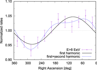
Figure 1. Distribution in R.A. of the normalized rates of events with energy above 8 EeV. The black solid and blue dashed lines show the distributions obtained from the weighted Fourier analysis corresponding to a first harmonic (χ2/dof = 1.02, for 10 degrees of freedom) and first plus second harmonics (χ2/dof = 0.44, for 8 degrees of freedom), respectively.
Download figure:
Standard image High-resolution imageIn Table 2, we report the results of the harmonic analysis in the azimuth angle. The  amplitudes, which give a measure of the difference between the flux coming from the east and that coming from the west, integrated over time, should vanish if there are no spurious modulations affecting the azimuth distribution. The values obtained are in fact compatible with zero in the two bins. The
  amplitudes, which give a measure of the flux modulation in the north–south direction, can be used to estimate the component of the CR dipole along Earth's rotation axis. The most significant amplitude is obtained for energies between 4 and 8 EeV and is
  , corresponding to an excess CR flux from the south, which has a chance probability to arise from an isotropic distribution of 0.009. Regarding the second harmonic, none of the amplitudes found are significantly different from zero.
Table 2. Results of the First- and Second-harmonic Analyses in Azimuth
| Energy (EeV) | k |

|

|

|

|
|---|---|---|---|---|---|
| 4–8 | 1 | −0.010 ± 0.005 | −0.013 ± 0.005 | 0.045 | 0.009 |
| 2 | 0.002 ± 0.005 | −0.002 ± 0.005 | 0.69 | 0.69 | |
| ≥8 | 1 | −0.007 ± 0.008 | −0.014 ± 0.008 | 0.38 | 0.08 |
| 2 | −0.002 ± 0.008 | 0.006 ± 0.008 | 0.80 | 0.45 | |
Download table as: ASCIITypeset image
Figure 2 displays the maps, in equatorial coordinates, of the exposure-weighted average of the flux inside a top-hat window of radius 45°, so as to better appreciate the large-scale features, for the energy bins [4, 8] EeV and E ≥ 8 EeV. An excess in the flux from the southern directions is the predominant feature at energies between 4 and 8 EeV, while above 8 EeV the excess comes from a region with R.A. close to 100°, with a corresponding deficit in the opposite direction, in accordance with the results from the harmonic analyses in R.A. and azimuth.
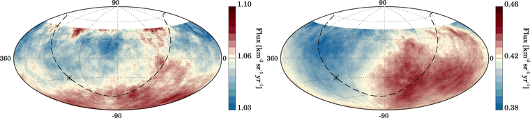
Figure 2. Maps in equatorial coordinates of the CR flux, smoothed in windows of 45°, for the energy bins [4, 8] EeV (left) and E ≥ 8 EeV (right). The Galactic plane is represented with a dashed line, and the Galactic center is indicated with a star.
Download figure:
Standard image High-resolution imageGiven the significant first-harmonic modulation in R.A. that was found in the bin with E ≥ 8 EeV, we now divide this higher-energy bin into three to study the possible energy dependence of this signal. For this, we use energy boundaries scaled by factors of two, i.e., considering the bins [8, 16] EeV, [16, 32] EeV, and E ≥ 32 EeV. Table 3 reports the results for the R.A. analysis in these new energy bins. The p-values for the first-harmonic modulation in R.A. are 3.7 × 10⁻⁶ in the [8, 16] EeV range, 0.014 in the [16, 32] EeV bin, and 0.26 for energies above 32 EeV. Table 4 reports the results for the corresponding azimuth analysis in these new energy bins.
Table 3. Results of the First-harmonic Analysis in R.A. in the Three Bins above 8 EeV
| Energy (EeV) | Events |

|

|

|
 (deg) (deg) |

|
|---|---|---|---|---|---|---|
| 8–16 | 24,070 | −0.011 ± 0.009 | 0.044 ± 0.009 | 0.046 | 104 ± 11 | 3.7 × 10⁻⁶ |
| 16–32 | 6604 | 0.007 ± 0.017 | 0.050 ± 0.017 | 0.051 | 82 ± 20 | 0.014 |
| ≥32 | 1513 | −0.03 ± 0.04 | 0.05 ± 0.04 | 0.06 | 115 ± 35 | 0.26 |
Download table as: ASCIITypeset image
Table 4. Results of the First-harmonic Analysis in Azimuth in the Three Bins above 8 EeV
| Energy (EeV) |

|

|

|

|
|---|---|---|---|---|
| 8–16 | −0.013 ± 0.009 | −0.004 ± 0.009 | 0.15 | 0.66 |
| 16–32 | 0.003 ± 0.017 | −0.042 ± 0.017 | 0.86 | 0.013 |
| ≥32 | 0.05 ± 0.04 | −0.04 ± 0.04 | 0.21 | 0.32 |
Download table as: ASCIITypeset image
3.2. Reconstruction of the CR Dipole
We now convert the harmonic coefficients in R.A. and in azimuth into anisotropy parameters on the sphere, assuming first that the dominant component of the anisotropy is the dipole  . The flux distribution can then be parameterized as a function of the CR arrival direction
  as
as

In this case, the amplitude of the dipole component along the rotation axis of Earth, dz, that in the equatorial plane, d⊥, and the R.A. and decl. of the dipole direction, (αd, δd), are related to the first-harmonic amplitudes in R.A. and azimuth through (The Pierre Auger Collaboration 2015b)
where  is the mean cosine of the decl. of the events,
  is the mean sine of the event zenith angles, and
  is the latitude of the observatory. Note that, as is well known, when the coverage of the sky is not complete, a coupling between the reconstructed multipoles can occur. The dipole parameters inferred from this set of relations can thus receive extra contributions from higher-order multipoles, something that will be explicitly checked in the next subsection in the case of a non-negligible quadrupolar contribution to the flux.
In the two upper rows of Table 5, we show the reconstructed dipole components for the energy bins previously studied, [4, 8] EeV and E ≥ 8 EeV. The results for the three new bins above 8 EeV are reported in the lower three rows. The uncertainties in the amplitude and phase correspond to the 68% confidence level (CL) of the marginalized probability distribution functions.
Table 5. Three-dimensional Dipole Reconstruction for Energies above 4 EeV
| Energy (EeV) | d⊥ | dz | d | αd (deg) | δd (deg) | |
|---|---|---|---|---|---|---|
| Interval | Median | |||||
| 4–8 | 5.0 |

|
−0.024 ± 0.009 |

|
80 ± 60 |

|
| ≥8 | 11.5 |

|
−0.026 ± 0.015 |

|
100 ± 10 |

|
| 8–16 | 10.3 |

|
−0.008 ± 0.017 |

|
104 ± 11 |

|
| 16–32 | 20.2 |

|
−0.08 ± 0.03 |

|
82 ± 20 |

|
| ≥32 | 39.5 |

|
−0.08 ± 0.07 |

|
115 ± 35 |

|
Note. We show the results obtained for the two bins previously reported (The Pierre Auger Collaboration 2017a), i.e., between 4 and 8 EeV and above 8 EeV, as well as dividing the high-energy range into three bins.
Download table as: ASCIITypeset image
In Table 5 a growth of the dipolar amplitude d with increasing energies is observed. Adopting for the energy dependence of the dipole amplitude a power-law behavior  , we perform a maximum likelihood fit to the values measured in the four bins above 4 EeV. We consider a likelihood function
  , where in each energy bin f is given by a 3D Gaussian for the dipole vector
  , centered at the measured dipole values and with the dispersions
  and
and  , marginalized over the angular variables α and δ. The fit leads to a reference amplitude d10 =0.055 ± 0.008 and a power-law index β = 0.79 ± 0.19.98
A fit with an energy-independent dipole amplitude (β = 0) is disfavored at the level of 3.7σ by a likelihood ratio test.
, marginalized over the angular variables α and δ. The fit leads to a reference amplitude d10 =0.055 ± 0.008 and a power-law index β = 0.79 ± 0.19.98
A fit with an energy-independent dipole amplitude (β = 0) is disfavored at the level of 3.7σ by a likelihood ratio test.
The left panel of Figure 3 shows the amplitude of the dipole as a function of the energy, with the data points centered at the median energy in each of the four bins above 4 EeV, as well as the power-law fit. The right panel is a map, in Galactic coordinates, showing the 68% CL sky regions for the dipole direction in the same bins. They all point toward a similar region of the sky, and in order of increasing energies they are centered at Galactic coordinates (ℓ, b) = (287°, −32°), (221°, −3°), (257°, −33°) and (259°, −11°), respectively. With the present accuracy no clear trend in the change of the dipole direction as a function of energy can be identified. In the background of Figure 3, we indicate with dots the location of the observed galaxies from the 2MRS catalog that lie within 100 Mpc and also show with a cross the reconstructed 2MRS flux-weighted dipole direction (Erdogdu et al. 2006), which could be expected to be related to the CR dipole direction if the galaxies were to trace the distribution of the UHECR sources and the effects of the magnetic field deflections were ignored.

Figure 3. Evolution with energy of the amplitude (left panel) and direction (right panel) of the 3D dipole determined in different energy bins above 4 EeV. In the sky map in Galactic coordinates of the right panel the dots represent the direction toward the galaxies in the 2MRS catalog that lie within 100 Mpc, and the cross indicates the direction toward the flux-weighted dipole inferred from that catalog.
Download figure:
Standard image High-resolution imageFigure 4 shows sky maps, in Galactic coordinates, of the ratio between the observed flux and that expected for an isotropic distribution, averaged in angular windows of 45° radius, for the different energy bins above 4 EeV. The location of the main overdense regions can be observed. Note that the color scale is kept fixed, so as to better appreciate the increase in the amplitude of the flux variations with increasing energies.

Figure 4. Maps in Galactic coordinates of the ratio between the number of observed events in windows of 45° and those expected for an isotropic distribution of arrival directions, for the four energy bins above 4 EeV.
Download figure:
Standard image High-resolution image3.3. Reconstruction of a Dipole plus Quadrupole Pattern
In order to quantify the amplitude of the quadrupolar moments and their effects on the dipole reconstruction, we assume now that the angular distribution of the CR flux can be well approximated by the combination of a dipole plus a quadrupole. In this case, the flux can be parameterized as

with Qij being the symmetric and traceless quadrupole tensor.
The components of the dipole and of the quadrupole can be estimated as in The Pierre Auger Collaboration (2015b). They are obtained from the first and second harmonics in R.A. and azimuth, given in Tables 1 and 2, as well as considering the first harmonic in R.A. of the events coming from the northern and southern hemispheres separately, which are reported in Table 6. From these results we obtained the three dipole components and the five independent quadrupole components that are reported in Table 7, for the two energy bins [4, 8] EeV and E ≥ 8 EeV. The only nonvanishing correlation coefficients between the quantities reported in Table 7 are  and
and  . The nine components of the quadrupole tensor can be readily obtained from those in Table 7 exploiting the condition that the tensor be symmetric and traceless. None of the quadrupole components are statistically significant, and the reconstructed dipoles are consistent with those obtained before under the assumption that no higher multipoles are present. They are also consistent with results obtained in past analyses in The Pierre Auger Collaboration (2015b) and The Pierre Auger & Telescope Array Collaborations (2014). Note that allowing for the presence of a quadrupole leads to larger uncertainties in the reconstructed dipole components, especially in the one along Earth's rotation axis due to the incomplete sky coverage present around the north celestial pole. Indeed, in both energy bins the uncertainties in the equatorial dipole components increase by ∼30%, while those on dz increase by a factor of about 2.7.
Table 6. Results of the First Harmonic in R.A., Separating the Events into Those Arriving from the Southern (S) and Northern (N) Hemispheres
| Energy (EeV) | Hemisphere | N |

|

|

|
 (deg) (deg) |
|---|---|---|---|---|---|---|
| 4–8 | S | 65,183 | 0.003 ± 0.005 | 0.005 ± 0.005 | 0.006 | 60 ± 50 |
| N | 16,518 | −0.009 ± 0.011 | 0.003 ± 0.011 | 0.010 | 160 ± 60 | |
| ≥8 | S | 25,823 | −0.011 ± 0.009 | 0.047 ± 0.009 | 0.048 | 103 ± 10 |
| N | 6364 | 0.0024 ± 0.018 | 0.041 ± 0.018 | 0.041 | 87 ± 25 | |
Download table as: ASCIITypeset image
Table 7. Reconstructed Dipole and Quadrupole Components in the Two Energy Bins
| Energy (EeV) | di | Qij |
|---|---|---|
| 4–8 | dx = −0.005 ± 0.008 | Qzz = −0.01 ± 0.04 |
| dy = 0.005 ± 0.008 |

|
|
|
|
|
| Qxz = −0.020 ± 0.019 | ||
| Qyz = −0.005 ± 0.019 | ||
| ≥8 | dx = −0.003 ± 0.013 | Qzz = 0.02 ± 0.06 |
| dy = 0.050 ± 0.013 | Qxx − Qyy = 0.08 ± 0.05 | |
|
|
|
| Qxz = 0.02 ± 0.03 | ||
| Qyz = −0.03 ± 0.03 | ||
Note. The x-axis lies in the direction α = 0.
Download table as: ASCIITypeset image
From the components of the quadrupole tensor it is possible to define an average quadrupole amplitude,  . This amplitude is directly related to the usual angular power spectrum moments Cℓ through
  , and it is hence a rotationally invariant quantity. From the results given in Table 7 one obtains that Q = 0.012 ± 0.009 for 4 ≤E/EeV < 8 and Q = 0.032 ± 0.014 for E ≥ 8 EeV. We note that for isotropic realizations, 95% of the values of Q would be below 0.037 and 0.060, respectively, showing that the quadrupole amplitude is consistent with isotropic expectations.
4. On the Dipole Uncertainties
Let us now discuss the impact of the different systematic effects that we have accounted for. The variations in the array size with time and the atmospheric variations are the two systematic effects that could influence the estimation of the equatorial component of the dipole. Had we neglected the changes in the array size with time, it would have changed d⊥, with the data set considered, by less than 4 × 10⁻⁴, and not performing the atmospheric corrections would have changed d⊥ by less than 10−3 (the precise amount of the change in these two cases depends on the particular phase of d⊥ in each energy bin). The small values of the effects due to atmospheric corrections and changes in the exposure are mostly due to the fact that for the present data set they are averaged over a period of more than 12 yr. On the other hand, the tilt of the array and the effects of the geomagnetic field on the shower development can influence the estimation of the north–south dipole component. The net effect of including the tilt of the array when performing observations up to zenith angles of 80° is to change dz by +0.004, which is small since the observatory site is in a very flat location. The largest effect is that associated with the geomagnetic corrections, which change dz by +0.011. Since these corrections are known with an uncertainty of about 25% (The Pierre Auger Collaboration 2011), they leave as a remnant a systematic uncertainty on dz of about 0.003.
A standard check to verify that all the systematic effects that can influence the right ascension distribution are accurately accounted for, in particular those arising from atmospheric effects or from the variations in the exposure of the array with time, is to look at the Fourier amplitude at the solar and anti-sidereal frequencies (Farley & Storey 1954). No significant physical modulation of CR should be present at these frequencies for an anisotropy of astrophysical origin. We report in Table 8 the results of the first-harmonic analysis at these two frequencies. One can see that the flux modulations at both the solar and anti-sidereal frequencies, having amplitudes with a sizable chance probability, are in fact compatible with zero for the two energy ranges considered.
Table 8. First-harmonic Amplitude, and Probability for It to Arise as a Fluctuation of an Isotropic Distribution, at the Solar and Anti-sidereal Frequencies
| Energy | Solar | Anti-sidereal | ||
|---|---|---|---|---|
| (EeV) | r1 |

|
r1 |

|
| 4–8 | 0.006 | 0.48 | 0.004 | 0.76 |
| ≥8 | 0.007 | 0.69 | 0.011 | 0.36 |
Download table as: ASCIITypeset image
Regarding the effects of possible systematic distortions in the zenith-angle distributions, such as those that could arise, for instance, from a mismatch between the energy calibration of vertical and inclined events, they could affect the dipole components by modifying the quantities  or
or  entering in Equation (5). Considering, for instance, the E ≥ 8 EeV bin, we note that for these events
  , while the expected value that is obtained from simulations with a dipolar distribution with amplitude and direction similar to the reconstructed one and the same number of events is
  (while an isotropic distribution would lead to a central value
  ). If the difference between the observed and the expected values of
  , which is less than 1%, were attributed to systematic effects in the zenith distribution, the impact that this would have on the inferred dipole component dz would be negligible in comparison to its statistical uncertainty, which is about 50%. Similarly, the value of the average decl. cosine in the data is
  , while that expected for the inferred dipole obtained through simulations is 0.7811 ± 0.0013, showing that possible systematic effects on d⊥ arising from this quantity are even smaller. This is a verification that the method adopted is largely insensitive to possible systematic distortions in the zenith or decl. distribution of the events.
5. Discussion
The most significant anisotropy in the distribution of CR observed in the studies performed above 4 EeV is the large-scale dipolar modulation of the flux at energies above 8 EeV. The maximum of this modulation lies in Galactic coordinates at (l, b) = (233°, −13°), with an uncertainty of about 15°. This is 125° away from the Galactic center direction, indicating an extragalactic origin for these ultrahigh-energy particles. As examples of the large-scale anisotropies expected from a Galactic CR component, we show in Figure 5 the direction of the dipole that would result for CR coming from sources distributed as the luminous matter in the Galaxy, taken as a bulge and an exponential disk modeled as in Weber & de Boer (2010). The CRs are propagated through the Galactic magnetic field, described with the models proposed in Jansson & Farrar (2012) and Pshirkov et al. (2011), for different values of the CR rigidity, R = E/eZ (with eZ the charge of the CR nucleus). The results are obtained by actually backtracking the trajectories of antiparticles leaving Earth (Thielheim & Langhoff 1968) from a dense grid of equally spaced directions and obtaining the associated weight for each direction by integrating the matter density along their path through the Galaxy (Karakula et al. 1972). We obtain in this way an estimation of the flux that would arrive at Earth from a continuous distribution of sources isotropically emitting CR and with a density proportional to that of the luminous matter. The points in the plot indicate the direction of the reconstructed dipolar component of the flux maps obtained. The directions of the resulting dipoles lie very close to the Galactic center for particles with the highest rigidities considered, and as the rigidity decreases, they slowly move away from it toward increasing Galactic longitudes (closer to the direction of the inner spiral arm, which is at (l, b) ≃ (80°, 0°)). Note that at 10 EeV the inferred average value of the CR charges is Z ∼ 1.7–5, depending on the hadronic models adopted for the analysis, while in the lower-energy bin the inferred charges are actually smaller (The Pierre Auger Collaboration 2014b), justifying the range of rigidities considered. The resulting dipole directions obtained in these Galactic scenarios are quite different from the dipole direction observed above 8 EeV, clearly showing that in a standard scenario the dominant contribution to the dipolar modulation at these energies cannot arise from a Galactic component. Besides the dipole direction, let us note that the amplitude of the dipole (and also the amplitudes of the quadrupole) turns out to be large in the models of purely Galactic CR (The Pierre Auger Collaboration 2012, 2013). In particular, we find that d > 0.8 for all the rigidities considered in the figure, showing that the dominant component at these energies needs to be much more isotropic, and hence of likely extragalactic origin.
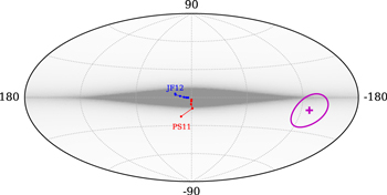
Figure 5. Map in Galactic coordinates of the direction of the dipolar component of the flux for different particle rigidities for CRs coming from Galactic sources and propagating in the Galactic magnetic field model of Jansson & Farrar (2012) (blue points) and the bisymmetric model of Pshirkov et al. (2011) (red points). The points show the results for the following rigidities: 64, 32, 16, 8, 4 and 2 EV (with increasing distance from the Galactic center). We also show in purple the observed direction of the dipole for E ≥ 8 EeV and the 68% CL region for it. The background in gray indicates the integrated matter density profile assumed for the Galactic source distribution (Weber & de Boer 2010).
Download figure:
Standard image High-resolution imageRegarding the possible origin of the dipolar CR anisotropy, we note that the relative motion of the observer with respect to the rest frame of CR is expected to give rise to a dipolar modulation of the flux, known as the Compton–Getting effect (Compton & Getting 1935). For particles with a power-law energy spectrum dΦ/dE ∝ E−γ, the resulting dipolar amplitude is  , with v/c the velocity of the observer normalized to the speed of light. In particular, if the rest frame of the CR were the same as that of the cosmic microwave background, the dipole amplitude would be dCG ≃ 0.006 (Kachelriess & Serpico 2006), an order of magnitude smaller than the observed dipole above 8 EeV. Thus, the Compton–Getting effect is predicted to give only a subdominant contribution to the dipole measured for energies above 8 EeV.
Plausible explanations for the observed dipolar-like distribution include the diffusive propagation from the closest extragalactic source(s) or that it be due to the inhomogeneous distribution of the sources in our cosmic neighborhood (Giler et al. 1980; Berezinsky et al. 1990; Harari et al. 2014, 2015). The expected amplitude of the resulting dipole depends in these cases mostly on the number density of the source distribution, ρ, with only a mild dependence on the amplitude of the extragalactic magnetic field.99
For homogeneous source distributions with  Mpc−3, spanning the range between densities of galaxy clusters, jetted radio galaxies, Seyfert galaxies, and starburst galaxies, the dipole amplitude turns out to be at the level of a few percent at E ∼10 EeV, both for scenarios with light (Harari et al. 2014) and with mixed CR compositions (Harari et al. 2015). A density of sources smaller by a factor of 10 leads on average to a dipolar amplitude larger by approximately a factor of two. An enhanced anisotropy could result if the sources were to follow the inhomogeneous distribution of the local galaxies, with a dipole amplitude larger by a factor of about two with respect to the case of a uniform distribution of the same source density. The expected behavior is exemplified in Figure 6, where we have included the observed dipole amplitude values together with the predictions from Harari et al. (2015) for a scenario with five representative mass components (H, He, C, Si, and Fe) having an E−2 spectrum with a sharp rigidity cutoff at 6 EV and adopting a source density ρ = 10−4 Mpc−3 (ignoring the effects of the Galactic magnetic field). The data show indications of a growth in the amplitude with increasing energy that is similar to the one obtained in the models. Note that this kind of scenario is also in line with the composition favored by Pierre Auger Observatory data (The Pierre Auger Collaboration 2017c).
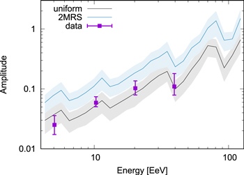
Figure 6. Comparison of the dipole amplitude as a function of energy with predictions from models (Harari et al. 2015) with mixed composition and a source density  . CRs are propagated in an isotropic turbulent extragalactic magnetic field with rms amplitude of 1 nG and a Kolmogorov spectrum with coherence length equal to 1 Mpc (with the results having only mild dependence on the magnetic field strength adopted). The gray line indicates the mean value for simulations with uniformly distributed sources, while the blue one shows the mean value for realizations with sources distributed as the galaxies in the 2MRS catalog. The bands represent the dispersion for different realizations of the source distribution. The steps observed reflect the rigidity cutoff of the different mass components.
Download figure:
Standard image High-resolution imageRegarding the direction of the dipolar modulation, it is important to take into account the effect of the Galactic magnetic field on the trajectories of extragalactic CR reaching Earth.100
The facts that the Galactic magnetic field model is not well known and that the CR composition is still uncertain make it difficult to infer the dipole direction associated with the flux outside the Galaxy from the measured one. As an example, we show in Figure 7 the change in the direction of an originally dipolar distribution after traversing a particular Galactic magnetic field, modeled in this example following Jansson & Farrar (2012). The arrows start in a grid of initial directions for the dipole outside the Galaxy and indicate the dipole directions that would be reconstructed at Earth for different CR rigidities. The points along the lines indicate the directions for rigidities of 32, 16, and 8 EV, and the tip of the arrow indicates those for 4 EV. We see that after traversing the Galactic magnetic field the extragalactic dipoles originally pointing in one half of the sky, essentially that of positive Galactic longitudes, tend to have their directions aligned closer to the inner spiral arm, at (l, b) ≃ (80°, 0°) (indicated with an  in the plot). On the other hand, those originally pointing to the opposite half tend to align their directions toward the outer spiral arm, at (l, b) ≃ (−100°, 0°) (indicated with an
  in the plot). The measured dipole direction for E ≥ 8 EeV is indicated with the shaded area, and one can see that it lies not far from the outer spiral arm direction. The line color shows the resulting suppression factor of the dipole amplitude after the effects of the Galactic magnetic field deflections are taken into account. Qualitatively similar results, showing a tendency for the direction of the dipolar component to align with the spiral arm directions, are also obtained when adopting instead the Galactic magnetic field from Pshirkov et al. (2011).

Figure 7. Change of the direction of the dipolar component of an extragalactic flux after traversing the Galactic magnetic field, modeled as in Jansson & Farrar (2012). We consider a grid (black circles) corresponding to the directions of a purely dipolar flux outside the Galaxy. Points along the lines indicate the reconstructed directions for different values of the particle rigidity: 32, 16, and 8 EV, and, at the tip of the arrow, 4 EV. The line color indicates the resulting fractional change of the dipole amplitude. The observed direction of the dipole for energies E ≥ 8 EeV is indicated by the gray plus sign, with the shaded area indicating the 68% CL region. The labels  and
and  indicate the directions toward the inner and outer spiral arms, respectively.
Download figure:
Standard image High-resolution imageThe detection of large-scale anisotropies could open the possibility to jointly probe the distribution of UHECR sources and that of extragalactic magnetic fields (Sigl et al. 2004). In particular, the growth of the dipole with energy is reproduced in the scenarios considered in Wittkowski & Kampert (2018), di Matteo & Tinyakov (2018), and Hackstein et al. (2018), which further investigate the expected strength of the quadrupolar moments, none of which is found to be significant in our study. In Wittkowski & Kampert (2018) actually the full angular power spectrum Cl up to l = 32 is obtained considering the mixed CR composition scenarios with a common maximum rigidity at the sources that best fit the Pierre Auger Observatory results (Wittkowski 2017). They found that only for l = 1, corresponding to the dipole, is the Cl expected to be greater than the 5σ CL range of isotropy when a number of events like that recorded by the Pierre Auger Observatory are considered. In di Matteo & Tinyakov (2018) the dipole and quadrupole amplitudes are examined under several assumptions on the mass composition, for a scenario of sources distributed as in the Two Micron All Sky Survey Galaxy Redshift Catalog. The amplitudes of the dipole moment reported in the present work can be well reproduced in their scenario with intermediate-mass nuclei. In Hackstein et al. (2018) pure proton or pure iron compositions and different magnetogenesis and source distribution scenarios are considered. For the proton case, the first multipole above 8 EeV is generally lower than the measured value (see also Hackstein et al. 2016), while a value closer to the observed one is obtained for the pure iron case. It is also concluded that UHECR large-scale anisotropies do not carry much information on the genesis and distribution of extragalactic magnetic fields. The dependence of the dipolar anisotropies on the rms amplitude and coherence length of a turbulent homogeneous intergalactic magnetic field was studied in Globus & Piran (2017), for proton, He, and CNO source models. They found that the dipole amplitudes for E ≥ 8 EeV turn out to be of the order of the one observed for a range of magnetic field parameters, and their model is consistent with an increase of the dipole amplitude with energy. In summary, the dipolar amplitude mostly depends on the large-scale distribution of the sources and their density, but it is not very sensitive to the details of the extragalactic magnetic field. Information on the extragalactic magnetic field parameters may eventually be obtained from the determination of anisotropies on smaller angular scales, for which a larger number of events would be needed.
6. Conclusions
We have extended the analysis of the large angular scale anisotropies of the CR detected by the Pierre Auger Observatory for energies above 4 EeV. The harmonic analyses both in R.A. and in azimuth allowed us to reconstruct the three components of the dipole under the assumption that the higher multipoles are subdominant. As already described in The Pierre Auger Collaboration (2017a), for the bin above 8 EeV the first-harmonic modulation in R.A. has a p-value of 2.6 × 10⁻⁸. The amplitude of the 3D reconstructed dipole is  for E ≥ 8 EeV, pointing toward Galactic coordinates (l, b) = (233°, −13°), suggestive of an extragalactic origin for these CRs. For 4 EeV ≤ E < 8 EeV the dipole amplitude is
  . Allowing for the presence of a quadrupolar modulation in the distribution of arrival directions, we determined here the three dipolar and the five quadrupolar components in the [4, 8] EeV and E ≥ 8 EeV bins. None of the quadrupolar components turned out to be statistically significant, and the dipolar components are consistent with the dipole-only results.
We also split the bin above 8 EeV into three to study a possible dependence of the dipole on energy. The direction of the dipole suggests an extragalactic origin for the CR anisotropies in each energy bin. We find that the amplitude increases with energy above 4 EeV, with a constant amplitude being disfavored at the 3.7σ level. A growing amplitude of the dipole with increasing energies is expected owing to the smaller deflections suffered by CR at higher rigidities. The dipole amplitude is also enhanced for increasing energies owing to the increased attenuation suffered by the CR from distant sources, which implies an increase in the relative contribution to the flux arising from the nearby sources, leading to a more anisotropic flux distribution.
Further clues to understand the origin of the UHECRs are expected to result from the study of the anisotropies at small or intermediate angular scales for energy thresholds even higher than those considered here. Also, the extension of the studies of anisotropies at large angular scales to lower energies may provide crucial information to understand the transition between the Galactic and extragalactic origins of CR.
The successful installation, commissioning, and operation of the Pierre Auger Observatory would not have been possible without the strong commitment and effort from the technical and administrative staff in Malargüe. We are very grateful to the following agencies and organizations for financial support:
Argentina—Comisión Nacional de Energía Atómica; Agencia Nacional de Promoción Científica y Tecnológica (ANPCyT); Consejo Nacional de Investigaciones Científicas y Técnicas (CONICET); Gobierno de la Provincia de Mendoza; Municipalidad de Malargüe; NDM Holdings and Valle Las Leñas, in gratitude for their continuing cooperation over land access; Australia—the Australian Research Council; Brazil—Conselho Nacional de Desenvolvimento Científico e Tecnológico (CNPq); Financiadora de Estudos e Projetos (FINEP); Fundação de Amparo à Pesquisa do Estado de Rio de Janeiro (FAPERJ); São Paulo Research Foundation (FAPESP) grant nos. 2010/07359-6 and 1999/05404-3; Ministério da Ciência, Tecnologia, Inovações e Comunicações (MCTIC); Czech Republic—grant no. MSMT CR LG15014, LO1305, LM2015038, and CZ.02.1.01/0.0/0.0/16_013/0001402; France—Centre de Calcul IN2P3/CNRS; Centre National de la Recherche Scientifique (CNRS); Conseil Régional Ile-de-France; Département Physique Nucléaire et Corpusculaire (PNC-IN2P3/CNRS); Département Sciences de l'Univers (SDU-INSU/CNRS); Institut Lagrange de Paris (ILP) grant no. LABEX ANR-10-LABX-63 within the Investissements d'Avenir Programme grant no. ANR-11-IDEX-0004-02; Germany—Bundesministerium für Bildung und Forschung (BMBF); Deutsche Forschungsgemeinschaft (DFG); Finanzministerium Baden-Württemberg; Helmholtz Alliance for Astroparticle Physics (HAP); Helmholtz-Gemeinschaft Deutscher Forschungszentren (HGF); Ministerium für Innovation, Wissenschaft und Forschung des Landes Nordrhein-Westfalen; Ministerium für Wissenschaft, Forschung und Kunst des Landes Baden-Württemberg; Italy—Istituto Nazionale di Fisica Nucleare (INFN); Istituto Nazionale di Astrofisica (INAF); Ministero dell'Istruzione, dell'Universitá e della Ricerca (MIUR); CETEMPS Center of Excellence; Ministero degli Affari Esteri (MAE); México—Consejo Nacional de Ciencia y Tecnología (CONACYT) no. 167733; Universidad Nacional Autónoma de México (UNAM); PAPIIT DGAPA-UNAM; The Netherlands—Ministry of Education, Culture and Science; Netherlands Organisation for Scientific Research (NWO); Dutch national e-infrastructure with the support of SURF Cooperative; Poland—National Centre for Research and Development, grant no. ERA-NET-ASPERA/02/11; National Science Centre, grant nos. 2013/08/M/ST9/00322, 2016/23/B/ST9/01635, and HARMONIA 5–2013/10/M/ST9/00062, UMO-2016/22/M/ST9/00198; Portugal—Portuguese national funds and FEDER funds within Programa Operacional Factores de Competitividade through Fundação para a Ciência e a Tecnologia (COMPETE); Romania—Romanian Ministry of Research and Innovation CNCS/CCCDI-UESFISCDI, projects PN-III-P1-1.2-PCCDI-2017-0839/19PCCDI/2018, PN-III-P2-2.1-PED-2016-1922, PN-III-P2-2.1-PED-2016-1659, and PN18090102 within PNCDI III; Slovenia—Slovenian Research Agency; Spain—Comunidad de Madrid; Fondo Europeo de Desarrollo Regional (FEDER) funds; Ministerio de Economía y Competitividad; Xunta de Galicia; European Community 7th Framework Program grant no. FP7-PEOPLE-2012-IEF-328826; USA—Department of Energy, contract nos. DE-AC02-07CH11359, DE-FR02-04ER41300, DE-FG02-99ER41107, and DE-SC0011689; National Science Foundation, grant no. 0450696; The Grainger Foundation; Marie Curie-IRSES/EPLANET; European Particle Physics Latin American Network; European Union 7th Framework Program, grant no. PIRSES-2009-GA-246806; and UNESCO.
Footnotes
- 96
The rms deflection of a particle of charge Z and energy E in a homogeneous turbulent magnetic field with rms amplitude B and coherence length lc is
 . For instance, oxygen nuclei with 30 EeV coming from a distance L ≃ 10 Mpc are deflected by about 30° for an extragalactic field of 1 nG, which is consistent with the bounds from cosmic background radiation and Faraday rotation measures (Durrer & Neronov 2013).
 - 97
The smaller but denser subarray with 750 m spacing among detectors is fully efficient down to ∼0.3 EeV for events with θ < 55°. The large-scale anisotropy results that can be obtained using it will be presented elsewhere.
- 98
Regarding the goodness of the fit, we have checked that, for a model in which the dipole amplitude follows the power law obtained, a better agreement than the one found with the actual data is expected to result in about 50% of the realizations.
- 99
This is because, as the value of the magnetic field is increased, for any given nearby source closer than the magnetic horizon its contribution to the CR density increases as it gets enhanced by the diffusion, while, on the other hand, the value of the dipolar component of its anisotropy decreases in such a way that both changes compensate for each other to a large extent.
- 100
These deflections not only can lead to a significant change in the dipole direction and in its amplitude but also can generate some higher-order harmonics even if pure dipolar modulation is only present outside the Galaxy (Harari et al. 2010).
