


Abstract
The large-scale distribution of globular clusters in the central region of the Coma cluster of galaxies is derived through the analysis of Hubble Space Telescope/Advanced Camera for Surveys data. Data from three different HST observing programs are combined in order to obtain a full surface density map of globular clusters in the core of Coma. A total of 22,426 Globular cluster candidates were selected through a detailed morphological inspection and the analysis of their magnitude and colors in two wavebands, F475W (Sloan g) and F814W (I). The spatial distribution of globular clusters defines three main overdensities in Coma that can be associated with NGC 4889, NGC 4874, and IC 4051 but have spatial scales five to six times larger than individual galaxies. The highest surface density of globular clusters in Coma is spatially coincidental with NGC 4889. The most extended overdensity of globular clusters is associated with NGC 4874. Intracluster globular clusters also form clear bridges between Coma galaxies. Red globular clusters, which agglomerate around the center of the three main subgroups, reach higher surface densities than blue ones.
Export citation and abstract BibTeX RIS
1. Introduction
The ability to detect extended stellar light with low surface brightness has changed our understanding and perception of galaxies. Mihos et al. (2005) obtained an extremely deep optical image of the Virgo cluster, revealing a striking and intricate web of intracluster light that has challenged our established view of the morphology of well studied galaxies such as M87, M86, and M84. Indeed, Mihos et al. (2005) revealed tails, bridges, and common envelopes between galaxies, a wealth of structure that had remained undetected until then.
Similar efforts to image faint stellar structures (μ ∼ 28 mag) have brought out tidal tails and stellar streams that show recent interactions of many galaxies (e.g., Malin & Hadley 1997; Martínez-Delgado et al. 2010). An interesting example of faint stellar structures in the Local Group revealed with deep wide-field imaging is given by the Pan-Andromeda Archaeological Survey (PAndAS, e.g., McConnachie et al. 2009; Ibata et al. 2014; Martin et al. 2014). PAndAS unveiled, for instance, structures that are the remnants of dwarf galaxies likely destroyed by the tidal field of M31. Studies of the H i line have also unveiled tidal tails and gas structures between interacting galaxies that are hidden to optical observations (Yun et al. 1994; López-Sánchez et al. 2012, among others).
Similar to intracluster light, intracluster globular clusters (IGCs) are generally defined as those globular clusters that are bound to the gravitational potential of a galaxy cluster instead of a particular galaxy. Observational hints and theoretical predictions of the existence of IGCs could be found in the literature more than three decades ago (Forte et al. 1982; Muzzio et al. 1984; White 1987, among others).
The unique sensitivity and resolution of the Advanced Camera for Surveys (ACS) on board the Hubble Space Telescope (HST) were instrumental in discovering and characterizing extragalactic globular cluster populations. First, with the WFPC2 and then with the ACS, a number of IGC detections were reported in Abell 1185 (Jordán et al. 2003; West et al. 2011), Virgo (Williams et al. 2007), and Abell 1689 (Alamo-Martínez & Blakeslee 2013). A tentative finding of IGCs in Fornax was also made by Bassino et al. (2003) using ground-based data.
The first detection of a large population of IGCs was made with SDSS data by Lee et al. (2010), who mapped the large-scale structure of IGCs in Virgo. Lee et al. (2010) found that globular clusters in Virgo define structures that are more extended than galaxies. From the maps made by Lee et al. (2010) it became obvious that a large fraction of globular clusters in Virgo are actually bound to the galaxy cluster potential instead of individual galaxies. A clear bridge of globular clusters between M87 and M86 is also evident (Lee et al. 2010). Durrell et al. (2014) expanded the work on Virgo using data from the Next Generation Virgo Cluster Survey.
In this paper, we present the results of a search for globular clusters in the central region of the Coma cluster carried out using HST data taken with the ACS. The existence and characteristics of IGCs in Coma were proven by Peng et al. (2011) and we build on their work by obtaining a larger field of view that is nearly continuous for the core of Coma.
The Coma cluster of galaxies, a nearby Abell cluster, consists of a massive population of diverse galaxies (e.g., Abell 1977; Colles & Dunn 1996). It has been the focus of intense study due in part to its high concentration of gravitationally bound objects, its extremely bright spiral galaxies and supermassive ellipticals NGC 4874 and NGC 4889 (Jørgensen et al. 1999; Boselli & Gavazzi 2006). Its close proximity to the north galactic pole of the Milky Way also allows for deep imaging of Coma unobscured by intermediate gas, dust, or foreground stars.
In the following sections, we discuss the HST observations we use, as well as our detection and selection criteria. We then present the color–magnitude diagram (CMD), the observed globular cluster luminosity function (GCLF), and the map of the large-scale structure formed by globular clusters in Coma. We obtain the surface brightness profiles of galaxies and compare them with the radial profiles of globular clusters. The spatial distribution of red and blue globular clusters is also shown. During this work, we create one of the largest globular clusters catalogs to date.
For this work a distance to the Coma cluster of 100 Mpc is adopted ((m − M) = 35.0 mag; Carter et al. 2008). This value yields a scale of 23 pc per 0 05, or one ACS pixel.
2. Advance Camera for Surveys Observations
We use HST Advance Camera for Surveys Wide Field Channel (ACS/WFC) data. Part of these public data were obtained during the ACS Coma Cluster Treasury Survey (GO 10861; Carter et al. 2008). We use the data products associated with data release 2.2 obtained from the Mikulski Archive for Space Telescopes at the STScI. We analyze the two bands obtained during the survey: F475W (Sloan g) and F814W (Cousins I). The exposure times for these data are 2677 s and 1400 s for the F475W and F814W filters, respectively. Further details of the ACS Survey on Coma can be found in Carter et al. (2008) and Peng et al. (2011). The photometric properties of these data, such as limiting magnitude, were presented by Hammer et al. (2010).
The ACS Coma cluster survey was planned to spatially cover the entire central region of Coma, but due to an electronics failure of the camera, the survey was not fully completed, leaving areas without imaging data. To compensate for these data gaps, additional archival HST pointings were analyzed. These are the green pointings in Figure 1. These additional pointings were obtained with the same filters under observing programs GO 11711 (PI: J. Blakeslee; Cho et al. 2016) and GO 12918 (PI: K. Chiboucas; Harris et al. 2017). By combining the imaging data of the programs above, we are able to finally study the central region of Coma as originally planned by the Coma Cluster Survey. A total of 25 ACS pointings were studied; each pointing has 2 filters. Compared with the study of Peng et al. (2011), we added seven additional pointings. These new pointings are crucial, as they include NGC 4889 and IC 4051. NGC 4889 is one of the two giant ellipticals in the core of Coma and its brightest galaxy (see Figure 1 and Table 1). IC 4051 is another giant elliptical on the outskirts of Coma that is known to have a large population of globular clusters (Woodworth & Harris 2000).
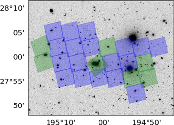
Figure 1. ACS pointings overlaid on an SDSS g-band image. The blue pointings were part of the study of Peng et al. (2011). For this work we include both blue and green pointings achieving a better coverage of the core of Coma. The green pointings were obtained under HST programs GO 11711 and GO 12918.
Download figure:
Standard image High-resolution imageTable 1. Properties of Coma Galaxies and GC Surface Density
| Galaxy | mV | Velocity | GC Surface |
|---|---|---|---|
| Name | (mag) | (km s−1) | Density |
| (N/''2) | |||
| IC 3973 | 14.37 | 4710 | 0.022 |
| IC 3976 | 14.70 | 6789 | 0.016 |
| IC 3998 | 14.57 | 9419 | 0.049 |
| IC 4011 | 15.12 | 7269 | 0.048 |
| IC 4012 | 14.94 | 7237 | 0.010 |
| IC 4021 | 14.85 | 5732 | 0.005 |
| IC 4026 | 14.59 | 8176 | 0.019 |
| IC 4030 | 15.40 | 7004 | 0.008 |
| IC 4033 | 15.21 | 7715 | 0.012 |
| IC 4040 | 14.84 | 7840 | 0.018 |
| IC 4041 | 14.35 | 7087 | 0.023 |
| IC 4045 | 13.94 | 6968 | 0.031 |
| IC 4051 | 13.63 | 8793 | 0.294 |
| NGC 4867 | 14.46 | 4822 | 0.034 |
| NGC 4869 | 13.76 | 6859 | 0.049 |
| NGC 4871 | 14.14 | 6795 | 0.080 |
| NGC 4872 | 14.41 | 7180 | 0.101 |
| NGC 4873 | 14.11 | 5824 | 0.137 |
| NGC 4874 | 11.68 | 7168 | 0.239 |
| NGC 4875 | 14.65 | 8008 | 0.048 |
| NGC 4876 | 14.39 | 6701 | 0.011 |
| NGC 4882 | 13.86 | 6371 | 0.283 |
| NGC 4883 | 14.35 | 8151 | 0.017 |
| NGC 4889 | 11.49 | 6446 | 0.477 |
| NGC 4894 | 15.19 | 4638 | 0.024 |
| NGC 4898 | 13.48 | 6661 | 0.049 |
| NGC 4906 | 14.10 | 7521 | 0.059 |
| NGC 4908 | 13.18 | 4903 | 0.063 |
Note. Properties of Coma galaxies and globular cluster surface density. Column (1): notable galaxies in Coma; column (2): galaxy total mV in magnitudes from de Vaucouleurs et al. (1991); column (3): radial velocity in km s−1 from NED; column (4): surface density of globular clusters at the position of the galaxy in numbers per arcsecond2.
Download table as: ASCIITypeset image
The definitive advantage of using high-resolution HST data is the ability to use morphology as an additional parameter to discriminate between globular clusters and other objects. Indeed, morphological information has been successfully used to differentiate between globular clusters and background galaxies at the distance of Coma (Peng et al. 2011). A subsection of this data set was also used to successfully identify ultra-compact dwarfs (UCDs) based on their photometry and morphology (Madrid et al. 2010).
3. Detection and Selection of Globular Cluster Candidates
Source detection is carried out using the task find within daophot. The final list of globular clusters candidates is achieved by analyzing their color, magnitudes, and size. A detailed account of the selection processes involved in creating the final list of globular cluster candidates is given in the Appendix.
Through detailed visual analysis of the properties of the candidates we produced a final list of globular cluster that is virtually free of contaminants such as background galaxies and artifacts. We stress that all globular clusters in the final list of candidates were validated through visual inspection by displaying the detections on the screen and scanning them on each image, and in both filters. We thus build a master catalog of 22,426 direct detections of globular cluster candidates in Coma.
4. Photometry and CMD
Flux measurements are derived using phot within daophot. Aperture photometry is carried out with phot using an aperture radius of 4 pixels. Aperture correction is applied using the prescription of Sirianni et al. (2005). We adopt a value of E(B − V) = 0.009 mag for the foreground galactic extinction. Photometric zero-points are obtained from the updated ACS zero-point tables maintained on the STScI website; we use ZPF475W = 26.131 mag and ZPF814W = 25.504 mag.
The CMD made with the final list of 22,426 globular cluster candidates is shown in Figure 2. This CMD is in good agreement with the magnitude and color distributions found in earlier work done with the HST on Coma globular clusters (Harris et al. 2009; Madrid et al. 2010; Chiboucas et al. 2011). A color histogram is presented above the CMD: 98.3% of all the globular cluster candidates have colors in the range  .
.

Figure 2. Color–magnitude diagram made with the final catalog of globular cluster candidates. The upper panel shows the color histogram, while the right panel shows the magnitude histogram or luminosity function.
Download figure:
Standard image High-resolution image5. GCLF
As mentioned by Peng et al. (2011), these data are too shallow to derive direct parameters for the GCLF. The histogram on the right side of the CMD is the observed GCLF in the F814W filter, as defined by our master catalog of candidates, reproduced in Figure 3. The peak of the histogram in Figure 3 is  mag (
mag ( = −9.5 mag). Most globular clusters (99.7%) have magnitudes in the range 20 ≤ mag ≤ 28, which translates into the absolute magnitude range of
  .
.
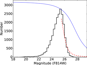
Figure 3. Observed globular cluster luminosity function (solid black histogram), and "completeness function" of our source finding routine (blue solid line). The red dashed line shows the fraction of detections that successfully pass our selection criteria. For instance, at  mag, 55% of all detected sources are classified as globular cluster candidates. The rejection rate increases with fainter magnitudes; at
  mag, only 13% of detections pass the selection criteria.
Download figure:
Standard image High-resolution imageThe turnover magnitude of the GCLF around bright ellipticals in Coma was determined to be about a magnitude fainter than the peak of the histogram in Figure 3. Using HST/WFPC2 with longer exposure times (of up to 31,200 s per filter), Harris et al. (2009) found a turnover magnitude of  mag for globular clusters in Coma. In the analysis of the GCLF in Virgo and Fornax Villegas et al. (2010) achieved results similar to those of Harris et al. (2009) in Coma.
The effectiveness of our detection algorithm is estimated by injecting artificial stars into the ACS files using the pyraf task addstar within daophot. Artificial stars with magnitudes between  mag and
  = 35 mag are added. One hundred artificial stars per magnitude bin of 0.5 mag are injected into the images. Adopting these values avoids overcrowding. We thus measure the fraction of artificial stars that are successfully recovered. We adopt the functional form of the completeness function defined by Harris et al. (2009):
where m0 is the completeness limit at which f reaches 50%, and α is the slope, which defines the rate at which f declines as it passes through m0 (Harris et al. 2009). This function is plotted in Figure 3 as a solid blue line with the following parameters: m0 = 27.62, and α = 0.48.
The "completeness function" derived above, only represents our ability to detect sources with our source finding algorithm. As detailed in the Appendix, only ∼25% of point sources initially detected on the HST images are classified as globular cluster candidates.
In order to illustrate the impact of our selection criteria on the observed GCLF, we plot in Figure 3, as a red dashed line, the fraction of detections that successfully pass our selection criteria and are classified as globular cluster candidates. This red dashed line has the same functional form as Equation (1), with the following parameters: m0 = 25.80 and α = 1.35. At  mag, 55% of all detected sources are classified as globular cluster candidates. The rejection rate increases with fainter magnitudes; at
  mag, only 13% of all detections pass the selection criteria. The design of these observations and our conservative selection criteria make the observed luminosity function presented in this section unsuitable for a detailed analysis of the GCLF parameters.
UCDs are considered to have magnitudes of  mag (Mieske et al. 2006). If we assume
  mag and the distance modulus of 35.0 mag quoted above, all sources in the master catalog with
  mag could be considered UCD candidates. Our catalog contains 867 UCD candidates, or 3.9% of the sample.
6. Wide-field Map of Globular Clusters in Coma
Surface density (or heat) maps are created using our final master catalog of globular clusters. These are made using the contourf routine of the Matplotlib library in Python. The contours use the ndimage.zoom routine from the Scipy library to interpolate and smooth the values. We use a spline interpolation of 4th order and a rescaling factor of two along each axis.
The heat map shown in Figure 4 shows that instead of simply belonging to a single parent galaxy, globular clusters outline the existence of a large-scale structure consistent with three main agglomerations.

Figure 4. Surface density of globular clusters in the central regions of the Coma cluster. This heat map defines three main overdensities of globular clusters in Coma. The highest density of globular clusters in Coma is cospatial with NGC 4889. The most extended agglomeration of globular clusters can be associated with NGC 4874. A third overdensity is associated with IC 4051. North is up and east is left.
Download figure:
Standard image High-resolution imageNGC 4874, NGC 4871, NGC 4872, and NGC 4873 appear to share a common envelope in one of the main agglomerations of globular clusters. Similarly, NGC 4889 and NGC 4882 are enshrouded by one common subgroup of globular clusters. In the core of Coma, globular clusters could be associated with several large galaxies instead of a single one. A third, less populous, agglomeration of globular clusters can be associated with IC 4051, which defines the third peak of the surface density of globular clusters.
The globular clusters associated with the IC 4051 overdensity form a rather symmetrical and elongated elliptical shape. The morphology of the two other overdensities located around the two cD galaxies is far more complex. These structures are clearly irregular and asymmetric.
Moreover, the distribution of globular clusters is different from the distribution of galaxies. There is a clear bridge of globular clusters between NGC 4889 and NGC 4874. This bridge was already visible in the work of Peng et al. (2011). The globular cluster overdensity cospatial with NGC 4889 extends southwest of NGC 4889 into a region where no large galaxies are present.
Table 1 lists the most notable galaxies in Coma, along with their apparent magnitudes and radial velocities in km s−1. This table also lists the value of the heat map at the location of each galaxy. The largest surface density of globular clusters in Coma, 0.477 GC arcsec−2, is spatially coincident with one of the two cD galaxies: NGC 4889. Interestingly, the second highest surface density corresponds to IC 4051 instead of the other cD, NGC 4874.
By studying a much wider field of view than Peng et al. (2011) we are able to reveal sections of the core of Coma where the surface density of globular clusters falls to ∼0. Figure 4 shows that NGC 4906 is isolated from the large-scale structure of globular clusters, despite continuous imaging coverage. Another section of the map virtually free of globular clusters is located between IC 4033 and IC 4041.
The heat map on Figure 4 shows that several bright galaxies are located in regions with low-surface-density globular clusters, i.e., have globular cluster systems with low numbers of members. Five clear examples of those bright galaxies associated with low numbers of globular clusters are IC 4021 (mV = 14.85 mag), IC 4030 (mV = 15.40 mag), IC 4033 (mV = 15.21 mag), IC 4040 (mV = 14.84 mag), and NGC 4876 (mV = 14.39 mag).
6.1. Spatial Scales of Globular Cluster Overdensities
We derive the radial profiles for the surface brightnesses of NGC 4874, NGC 4889, IC 4051, and their associated globular clusters, as shown in Figure 5. In order to quantify the spatial scales of both galaxy light and globular clusters, we fit a single Sérsic model to their radial profiles. We note that an exhaustive analysis of the surface brightness profile for these galaxies is beyond the scope of this paper. We fit a Sérsic model with the aim of obtaining a characteristic effective radius only. The effective radius of the Sérsic model is derived using the prescriptions of Graham & Driver (2005). The results of this analysis are given in Table 2.
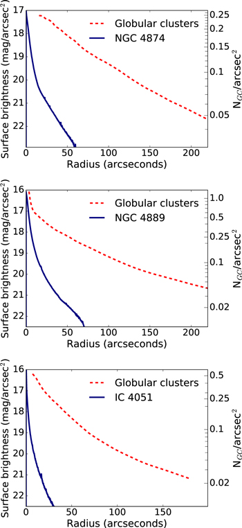
Figure 5. Surface brightness profiles of NGC 4874, NGC 4889, and IC 4051, and radial density profiles of globular clusters associated with these three overdensities. Globular clusters have radial distributions five to six times more extended than the light of individual galaxies—see also Table 2.
Download figure:
Standard image High-resolution imageTable 2. Effective Radii
| Galaxy | Galaxy Surface | Globular Clusters |
|---|---|---|
| Brightness Profile | Radial Profile | |
| (arcsec) | (arcsec) | |
| NGC 4874 | 19.4 | 105.0 |
| NGC 4889 | 15.3 | 91.0 |
| IC 4051 | 8.2 | 45.6 |
Note. Column (1): galaxy name; column (2): effective radii of the galaxy's surface brightness profile (arcsec); column (3): effective radii of globular clusters radial profiles (arcsec).
Download table as: ASCIITypeset image
The spatial scales defined by the distribution of globular clusters are larger than the radius of any individual galaxy. As shown in Figure 5 and Table 2, globular clusters associated with NGC 4874 have an extended spatial structure with an effective radius that is more than five times the effective radius of the galaxy light. The NGC 4874 overdensity of globular clusters is the largest in the core of Coma—larger than the overdensity associated with NGC 4889 or IC 4051.
7. Distribution of Red and Blue Globular Clusters
Globular clusters are often classified as a function of their color as red or blue. These colors are in turn associated with metallicity, with blue globular clusters considered metal-poor and red deemed metal-rich (Zinn & West 1984; Larsen et al. 2001). Several studies of individual galaxies have shown that blue globular clusters have a more extended spatial distribution than red ones (Kundu et al. 1999; Larsen et al. 2001). Bassino et al. (2006) confirmed that red and blue globular clusters have different radial distributions at large distances (∼200 kpc) from their host galaxies by studying Fornax (NGC 1399) using wide-field photometry.
Lee et al. (2010) showed that blue IGCs form a more extended distribution than red ones in the Virgo Cluster, as did Bassino et al. (2006) with Fornax. We investigate the distribution of red and blue globular clusters in Coma by separating globular clusters with colors redder and bluer than  .
.
The choice of color separation above is an estimate based on the fact that the bright end of the color distribution of globular clusters around NGC 4874 can be fit with two Gaussians. These two Gaussians intersect at  = 1.61 (Madrid et al. 2010). If one accounts for ∼0.1 mag for the blue tilt of bright, metal-poor globular clusters (e.g., Peng et al. 2009), the dividing line between red and blue globular clusters can be set at
  . Given that the vast majority of globular clusters in our sample (98.3%) have colors between
  , the value
  is also a simple even separation.
The surface density distribution of red and blue globular clusters is presented in Figure 6. Red globular clusters are 52% of the sample; the remaining 48% are blue. In Coma, red globular clusters reach much higher surface densities than blue ones. Indeed, the highest surface density for blue clusters is 0.10 GC/''2, while this value reaches 0.41 GC/''2 for red clusters. Red GCs define high surface density clumps around the main subgroups of globular clusters associated with NGC 4889, NGC 4874, and IC 4051.
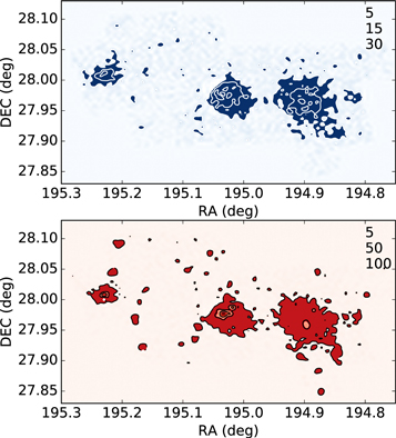
Figure 6. Surface density of blue (top) and red (bottom) globular clusters in the central region of the Coma cluster. The red globular clusters have higher surface densities than blue ones. Isocontour values are given in the top right corner. For a comparison with simulations see Ramos-Almendares et al. (2018).
Download figure:
Standard image High-resolution image8. Summary and Final Remarks
Globular clusters are distributed following three main overdensities in the core of Coma. The most extended overdensity is associated with NGC 4874, while the highest surface density of globular clusters is cospatial with NGC 4889. The second highest surface density of globular clusters coincides with IC 4051. The spatial distribution of globular clusters around NGC 4874, NGC 4889, and IC 4051 is five to six times more extended than the corresponding galaxy light.
The wide-field map of globular clusters presented here can be used in future work to investigate the evolutionary history of the Coma cluster by comparing it with numerical simulations like the one recently published by Ramos-Almendares et al. (2018).
This work shows what can be achieved when combining high-sensitivity, high resolution, and a wide field of view. WFIRST will have a sensitivity comparable to the HST and a much wider field of view that will allow us to image the entirety of galaxy clusters, such as Coma, with a single pointing.
We thank the anonymous referee for prompt and constructive reports. This work is based on observations made with the NASA/ESA HST, obtained at the Space Telescope Science Institute, which is operated by the Association of Universities for Research in Astronomy, Inc., under NASA contract NAS5-26555. These observations are associated with programs GO 10861, 11711, 12918. This research has made use of the NASA Astrophysics Data System Bibliographic services (ADS) and the NASA/IPAC Extragalactic Database (NED). A.G. acknowledges the funding of the National Science Foundation through the Research Experience for Undergraduates (REU) program, grant AST-1062976. C.O. acknowledges the support of an Australian Gemini Undergraduate Summer Studentship from the Australian Astronomical Observatory funded by Astronomy Australia Ltd.
This work uses SDSS imaging data. Funding for the SDSS and SDSS-II has been provided by the Alfred P. Sloan Foundation, the Participating Institutions, the National Science Foundation, the U.S. Department of Energy, the National Aeronautics and Space Administration, the Japanese Monbukagakusho, the Max Planck Society, and the Higher Education Funding Council for England. The SDSS website is http://www.sdss.org/.
Appendix
This appendix gives additional details on how the final sample of globular clusters is built. Table 3 summarizes the main steps taken to create the final catalog of globular clusters in Coma. The selection of globular cluster candidates is based on their photometric properties and sizes.
Table 3. Selection Criteria
| Step | Selection Criterion | Visual | Number |
|---|---|---|---|
| Inspection? | of Sources | ||
| Detection | |||
| 1 | First round of detections with DAOPHOT | Yes | 95785 |
| 2 | Remove spurious detections around edges and ACS chip gap | Yes | 80618 |
| 3 | Remove false detections near galaxy centers (inner few arcseconds) | Yes | 62882 |
| Color selection | |||
| 4 | Run daophot to create a Color–Magnitude Diagram | No | ⋯ |
| 5 | Inspect color outliers (i. e. outside  ) ) |
Yes | 50669 |
| Size selection | |||
| 7 | Run source extractor to determine sizes | No | ⋯ |
| 8 | Match sourcextractor and daophot catalogs, create size–magnitude plot | No | ⋯ |
| 9 | Second inspection of sources outside  pixels pixels |
Yes | 30328 |
| Final verification | |||
| 10 | Final visual verification | Yes | 23271 |
| Final sample 22426 | |||
Download table as: ASCIITypeset image
A.1. Source Finding
The first step is to run daofind, within daophot, to detect all sources at 1.8σ above the background. This value is determined through an iterative process. It is fine-tuned, by trial and error, to over-detect sources and ensure that all potential globular clusters are selected. False positives are removed a posteriori (see Figure 7). The second step consisted of identifying and removing spurious detections along the edges, and along the ACS chip gap.
For some bright galaxies daofind makes a large number of source detections around their centers. A steep gradient of galaxy light is often mistaken as a source by daofind. To circumvent this daofind issue, all detections within a few arcseconds of the center of bright galaxies are removed. Detections of true globular cluster candidates are then re-added by hand. For these inner regions of bright galaxies, we also use the median-subtracted images to better identify globular cluster candidates on the ds9 display. The median-subtracted images are produced using the commands median and imarith, the latter to subtract the median from the original image. We run find on the original and median-subtracted images, and both sets of detections are then cross-matched to create a master list of detections.
A.2. Color Selection
Once the photometry is obtained for the preliminary list of detections, a preliminary CMD is made. The CMDs of extragalactic globular cluster systems are well studied, beginning with the work done by Larsen et al. (2001). On that earlier work, Larsen et al. (2001) established a selection criteria for the color of globular clusters of  (translating into
 ![$-2.2\lt [{Fe}/H]\lt 0.2$](https://content.cld.iop.org/journals/0004-637X/867/2/144/revision1/apjaae206ieqn23.gif) ). Peng et al. (2006) selected objects with the color range
). Peng et al. (2006) selected objects with the color range  for their study of color distributions of globular clusters in Virgo.
An initial CMD allows us to build a list of objects that need secondary visual inspection due to suspicious colors or magnitudes, such as being very red or blue, or overly bright or faint. Candidates with colors redder than  and bluer than
  received a secondary inspection. Suspicious detections are displayed on the images and evaluated on individual grounds. To give a crude example, globular clusters in Coma should not have spiral arms, or show visible elongation on the ACS images. Some background galaxies can be easily picked up because of their colors. As shown in Figure 2, the vast majority of globular clusters have colors in the following range:
  . Sources with colors redder than
  are also excluded from the master catalog, given that these are likely high-redshift objects. Deriving flux measurements also allows us to remove a few detections that have bad (e.g., negative) fluxes.
A.3. Size Selection
As mentioned above, morphology is a powerful tool to discriminate between globular clusters and interlopers, especially when using high-resolution data. Before we do our morphological analysis, a PSF is derived by identifying several stars in the fields, obtaining their photometry and then running the PyRAF tasks pstselect and psf. The ACS/WFC PSF has a FWHM of ∼2 pixels. At the distance of Coma, globular clusters appear as point sources on the ACS images. Most globular clusters have radii of ∼3 pc, that is, are unresolved at the distance of Coma with a FHWM of ∼2 pixels. Great care is taken to preserve UCDs in our sample. Indeed, UCDs are slightly resolved at the distance of Coma with FWHM between ∼2 and ∼3 pixels.
To help with narrowing the list of globular cluster candidates, we derive the sizes of our detections using Sextractor (Bertin & Arnouts 1996). With the morphological information, a list of sources that are either too small (FWHM < 1.8 px) or too big (FWHM > 3.0 px) is created for inspection on the images; see the size–magnitude diagram shown in Figure 8. As mentioned above, globular clusters have sizes similar to the instrumental PSF. Most of the detections with sizes smaller than the PSF (e. g. ∼0.1 pixels) are cosmic rays. Similarly, large objects are usually background galaxies that have radii of tens or hundreds of pixels. Madrid et al. (2010) gave an example of background galaxies, present in this data set, that can be easily spotted by running a basic size estimate.
A.4. Final Verification
We then conduct a careful manual inspection of every remaining GC candidate. This is done with the help of the PyRAF task imexam, which we use to display intensity contours and 3D mapping (surface wire-plot) of the point sources. We also use imexam to derive the radial profile of globular cluster candidates and obtain an approximate size, which is compared to the PSF. Figure 7 shows a sample ACS pointing where we show all the original and final detections.
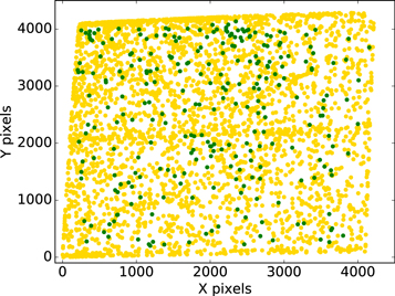
Figure 7. ACS pointing where we show all our original detections (in yellow) and the remaining globular clusters (in green) after down selection.
Download figure:
Standard image High-resolution image
Figure 8. Size–magnitude diagnostic plot for a sample pointing. Red sources are displayed on the images for further scrutiny. Sources with a FWHM ∼ 0 are almost invariably cosmic rays and other detector blemishes.
Download figure:
Standard image High-resolution image