


Abstract
The details of the physical mechanism that drives core-collapse supernovae (CCSNe) remain uncertain. While there is an emerging consensus on the qualitative outcome of detailed CCSN mechanism simulations in 2D, only recently have high-fidelity 3D simulations become possible. Here we present the results of an extensive set of 3D CCSN simulations using high-fidelity multidimensional neutrino transport, high-resolution hydrodynamics, and approximate general relativistic gravity. We employ a state-of-the-art 20 M☉ progenitor generated using Modules for Experiments in Stellar Astrophysics, and the SFHo equation of state. While none of our 3D CCSN simulations explode within ∼500 ms after core bounce, we find that the presence of large-scale aspherical motion in the Si and O shells aid shock expansion and bring the models closer to the threshold of explosion. We also find some dependence on resolution and geometry (octant versus full 4π). As has been noted in other recent works, we find that the post-shock turbulence plays an important role in determining the overall dynamical evolution of our simulations. We find a strong standing accretion shock instability (SASI) that develops at late times. The SASI produces transient shock expansions, but these do not result in any explosions. We also report that for a subset of our simulations, we find conclusive evidence for the lepton-number emission self-sustained asymmetry, which until now has not been confirmed by independent simulation codes. Both the progenitor asphericities and the SASI-induced transient shock expansion phases generate transient gravitational waves and neutrino signal modulations via perturbations of the protoneutron star by turbulent motions.
Export citation and abstract BibTeX RIS
1. Introduction
At the ends of their lives, stars more massive than about 8–10 M☉ develop inert, neutrino-cooled iron cores in their centers. The iron core in such stars builds up over a period of days due to core silicon burning and, ultimately, silicon shell burning until it reaches the effective Chandrasekhar mass, which in general depends on the electron fraction, Ye, and entropy of the core (Woosley et al. 2002). Once the iron core reaches this critical mass, gravitational collapse ensues. The collapse of the core is accelerated by electron captures onto nuclei and protons, the rates of both of which increase as the collapse drives the densities, and therefore the electron chemical potential higher and higher. The collapse accelerates to an appreciable fraction of the speed of light. The inner 0.5 M☉ of the core is in sonic contact and collapses homologously while the remaining outer core collapse supersonically. Electron-type neutrinos produced by the rapid electron captures are eventually "trapped" in the inner core once densities exceed about 1012 g cm−3. When the collapsing core reaches nuclear densities the residual strong force, also known as the nuclear force, between the nucleons starts to dramatically resist the force of gravity. This halts the collapse of the inner core, which then elastically rebounds and launches a pressure wave that quickly steepens into the supernova shock. The supernova shock propagates out into the still-infalling outer core leaving in its wake a hot protoneutron star (PNS). Energy losses from neutrino emission in the hot layers of the PNS and from the dissociation of the iron-group nuclei at the shock cause the shock to initially stall and become an accretion shock. At this time, the beginnings of neutrino-driven convection in the neutrino-heated, convectively unstable layers behind the supernova shock break the spherical symmetry that has otherwise dominated the evolution so far. These multidimensional instabilities are thought to be the crucial piece of the puzzle that assists the canonical explosion mechanism, the neutrino mechanism (Bethe & Wilson 1985), to reenergize the supernova shock and drive the supernova explosion.
Tremendous progress in the theoretical study of the core-collapse supernova (CCSN) mechanism has been made in recent years. This progress has been spurred largely by the advent of high-fidelity fully 3D simulations that can both capture the crucial hydrodynamic instabilities that form soon after core bounce and model the detailed neutrino transport that drives the thermodynamic evolution of the PNS and the shock-heating layers. (Hanke et al. 2013; Lentz et al. 2015; Melson et al. 2015b, 2015a; Roberts et al. 2016; Ott et al. 2018; Summa et al. 2018). Three-dimensional simulations also allow for the ability to directly simulate precollapse progenitor asphericities. At the point of collapse and outside of the iron core, there are shells of lighter elements. Immediately outside the iron core there is typically silicon shell that is undergoing nuclear burning that may or may not be convective at the point of core collapse, depending on the preceding evolution (e.g., Chieffi & Limongi 2013; Sukhbold & Woosley 2014), above this silicon shell is an oxygen shell that is also typically convective. Convection in these shells imprints nonspherical density structure and velocity motions on the progenitor. These are thought to be crucial for not only correctly simulating the core-collapse evolution, but perhaps needed in order to obtain explosions themselves. Evidence of this was seen as early as the 2D work of Burrows & Hayes (1996), but Couch & Ott (2013) were the first to show definitively on the basis of 3D simulations that nonspherical structure in the shells surrounding the collapsing iron core could qualitatively alter the outcome of CCSN simulations. Müller & Janka (2015) also showed, using parameterized precollapse perturbations in 2D simulations, that progenitor asphericities can play a strong role in the development of turbulence and lateral kinetic energy in the gain region, which boosts the effectiveness of neutrino heating, supports a larger shock radius, and helps drive explosions. Going beyond parameterized, artificially imposed perturbations, Couch et al. (2015) simulated the final few minutes of evolution through iron core collapse in a 15 M☉ star, directly calculating several convective turnover times in the Si-burning and O-burning shells. The resulting CCSN mechanism simulations with this 3D progenitor model showed a modest increase in the strength of the explosion, though not the strong qualitative impact found by Couch & Ott (2013). Subsequently, Müller et al. (2016) simulated a longer period of evolution through core collapse in an 18 M☉ star, finding substantial large-scale nonspherical motion in the O-burning shell. CCSN mechanism simulations with this progenitor (Müller et al. 2017) showed a dramatic impact from the realistic 3D progenitor, yielding a successful explosion for a case in which the comparable 1D progenitor failed.
In this work, we contribute new FLASH, high-resolution, full 3D, energy-dependent, three-species neutrino-radiation-hydrodynamic simulations of a 20 M⊙ zero-age main sequence (ZAMS) mass progenitor star evolved using the Modules for Experiments in Stellar Astrophysics (MESA; Paxton et al. 2011, 2013, 2015, 2018; Farmer et al. 2016) software. In our eight 3D simulations, we explore not only the 3D evolution of this progenitor, but we also explore the impact of progenitor asphericities, resolution, octant/full 3D symmetry, dimensionality, and variations in the evolution due to the neutrino transport physics. We do not obtain explosions in any of our 3D simulations, however we are able to quantitatively comment on the impact of each of the above aspects on the explosion mechanism. Our precollapse progenitor asphericities, particularly those in the silicon shell, are very effective at driving the development of turbulence in the post-shock layers. While only transitory in nature, this leads to larger average shock radii, more neutrino heating, and stronger turbulence. In the majority of our full 3D simulations we see the presence of the standing accretion shock instability (SASI). While this arises only once the supernova explosion is seemingly failing, we note that the growth of the SASI at late times can lead to epochs of shock reenergization. Unfortunately, these excursions are never large enough to drive an explosion in the time we have simulated. We see an imprint of the SASI motion on the neutrino luminosities. In one of our full 3D simulations we find a strong presence of the lepton-number emission self-sustained asymmetry (LESA). The LESA was first seen in Tamborra et al. (2014), but until now, has yet to be confirmed by other simulation codes. Lastly, we report on the gravitational wave signatures from all of our full 3D simulations. We find that the accretion of progenitor asphericities excite the PNS and lead to the temporary growth of the gravitational wave strength, as does the collapse of SASI spiral waves. The presence of such features in an observation of a nearby CCSNe may be a unique signal to the presence of strong transient turbulence in the accretion flow.
This paper is organized as follows. In the next section, Section 2, we introduce the FLASH code and describe the hydrodynamics, gravity, and neutrino transport. We also discuss our initial conditions and the parameterization we use for our precollapse progenitor asphericities. In Section 3, we first present an overview of our eight 3D simulations, contrasting them against each other. We explore in detail the nature of the presence of the SASI and the LESA. We also present the neutrino and gravitational wave signals from our simulations. We discuss and conclude in Section 4.
2. Methods
2.1. Hydrodynamics and Gravity
We make use of the FLASH hydrodynamics framework (Fryxell et al. 2000; Dubey et al. 2009) that we have outfitted for CCSNe in Couch (2013a, 2013b), Couch & O'Connor (2014), and more recently, have included both multidimensional, energy-dependent neutrino-radiation transport based on the moment formalism and effective general relativistic gravity in O'Connor & Couch (2018). For these simulations we use FLASH's unsplit hydrodynamic solver, which makes use of the piecewise parabolic method (Colella & Woodward 1984) and the hybrid HLLC Riemann solver, which reduces to HLLE in the presence of shocks. During each FLASH timestep, we solve for the new hydrodynamic state (the (n + 1) state) before the neutrino transport step. We refer the reader to previous works for a summary of the hydrodynamics and gravity methods (Couch 2013a, 2013b; Couch & O'Connor 2014; O'Connor & Couch 2018) and instead focus on a presentation of the multidimensional neutrino transport.
2.2. Neutrino Transport
Neutrinos play a critical role in CCSNe. First and foremost, they provide a tremendous cooling channel for the newly formed PNS, they also are a source of heat in the shocked layers above the PNS, the so-called gain region. This heat source is thought to be critical for the development of the explosion. Following the evolution of the neutrinos from the core of the PNS out through the gain region requires a complex treatment of neutrino-radiation transport. Furthermore, since the opacity of the matter has a strong dependence on the neutrino energy, this transport must be done in an energy-dependent way. In FLASH, we have implemented a multidimensional, multispecies, energy-dependent two-moment (with an analytic closure) neutrino-radiation transport scheme. It is based on the work of O'Connor (2015), Shibata et al. (2011), and Cardall et al. (2013). We have outlined our FLASH implementation in great detail in O'Connor & Couch (2018). For the majority of our 3D simulations presented here, we ignore the velocity dependence of the neutrino transport equations (i.e., we set  and its derivatives to 0). We also ignore the gravitational redshift term that moves neutrinos between energy bins, although we keep the overall source term from the gravitational redshift. These approximations are due to not having fully implemented this physics prior to beginning our 3D simulations. For comparison purposes, we do perform two simulations with full velocity and gravitational redshift dependence, which were started after these improvements were made to our neutrino transport code. For completeness, we show the form of our moment evolution equations here and refer the reader to the Appendix of O'Connor & Couch (2018) for implementation details. The coordinate frame, energy-dependent, neutrino energy density (E; zeroth moment) evolution equation in Cartesian coordinates is given as

and the coordinate frame, energy-dependent, neutrino momentum density (Fi; first moment) evolution equation is

where in these equations,  is the matter velocity (with the associated Lorentz factor of W);
  is the lapse (with ϕ being the gravitational potential), ν and ∂ν denote the neutrino energy and the energy-space derivative; κa, κs, and η are the matter absorption opacity, scattering opacity, and emissivity, respectively; Pij is the second moment of the neutrino distribution function, that we use an analytic closure for; Lij and Nijk are higher moment tensors used in the energy-space flux determination; and J and Hi are the fluid-frame zeroth and first moments that can be expressed in terms of E, Fi, and Pij,


These equations are energy and species dependent. We use 12 energy groups and three neutrino species (νe,  , and
, and  ). This amounts to 144 evolution equations. Since we perform the spatial flux and energy flux calculations explicitly, these differential equations are only coupled within an energy group and spatial zone. We perform the resulting 4 × 4 matrix inversions analytically.
The neutrino-matter interaction coefficients, κa, κs, and η are also energy and species dependent. They also depend on the matter density, temperature, and electron fraction. We use NuLib (O'Connor 2015) to generate a three-dimensional table (in density, temperature, and electron fraction), which we then tri-linearly interpolate, for each energy group and species, on the fly using the  -state matter variables from the hydrodynamic step. For the underlying neutrino interactions, we use isotropic scattering on nucleons, alpha particles, and heavy nuclei following Bruenn (1985) and Burrows et al. (2006), with corrections for weak magnetism and recoil from Horowitz (2002). For emission and absorption processes involving electron-type neutrinos and antineutrinos, we employ charged current interactions on neutron, protons, and heavy nuclei, specifically,


from Bruenn (1985) using weak magnetism and recoil corrections from Horowitz (2002). Finally, for thermal pair processes we use both electron–positron annihilation and nucleon–nucleon bremsstrahlung following Burrows et al. (2006) as implemented in O'Connor (2015). We only include these processes for heavy-lepton neutrinos.
2.3. Initial Conditions
For our suite of 3D simulations, we adopt the 20 M⊙, solar metallicity progenitor model from Farmer et al. (2016) produced using a non-equilibrium 204 isotope nuclear network with MESA (Paxton et al. 2011, 2013, 2015, 2018). We use the SFHo nuclear equation of state (EOS) (O'Connor & Ott 2010; Hempel et al. 2012; Steiner et al. 2013) everywhere. We simulate the collapse phase and early (first 15 ms) post-bounce phase using GR1D (O'Connor 2015) and then transition to FLASH. We use the same EOS table and neutrino interactions as well as the same description of gravity (i.e., using a general relativistic (GR) effective potential instead of full GR). We do interpolate from the 18 energy groups used in GR1D to the 12 energy groups used in the 3D FLASH simulations. We see a very smooth transition between the codes with little to no sign of transients that could impact the future evolution.
It is worth discussing the MESA 20 M⊙ progenitor and comparing it to another model frequently used in the literature. The 20 M⊙ MESA model (referred to as MESA20) is fairly similar to the 20 M⊙ model from Woosley & Heger (2007) (referred to here as s20). The compactness (ξM; O'Connor & Ott 2011) of the two 20 M⊙ models are also similar:  and
and  . The silicon–oxygen interface, where a sharp drop in density occurs (∼50% is both models), is located at a radius of ∼2400 km and ∼2600 km for MESA20 and s20, respectively. The baryonic mass coordinates of these interfaces are ∼1.75 M⊙ and ∼1.8 M⊙, respectively. In summary, the similarity of these properties results in a qualitative and quantitatively similar evolution of the mass accretion rate onto the PNS throughout the post-bounce phase.
We simulate the post-bounce phase in 3D using a Cartesian grid with adaptive mesh refinement. Our smallest grid zones are ∼488 m. The adaptive mesh refinement would ensure that all of the post-shock region is fully refined, however, for our baseline simulations we limit the refinement so as to only maintain a minimum effective angular resolution of Δx/r ≲0.009 or Δx/r ≲ 0 53. This restriction leads to a reduction in resolution from Δx ∼ 488 m to Δx ∼ 1 km at r ∼ 108 km, and further reduction by a factor of 2 at r ∼ 216 km. We refer to this as our standard resolution. We also have lower resolution simulations (denoted by LR in the model name) where we still take the smallest Δx = 488 m, but only enforce Δx/r ≲ 0.015 or Δx/r ≲ 088. This leads to the first resolution decrement at r ∼ 65 km, and subsequent decrements at r ∼ 130 km, r ∼ 260 km, etc. Our baseline simulations are full 3D (4π), however we perform some simulations in octant symmetry (denoted by oct in the model name). For two of our simulations we use an improved neutrino transport that includes full velocity dependence. We denote these simulations with a v in the model name. Finally, in two of our simulations we introduce velocity perturbations into the silicon and oxygen shell at the time of mapping to FLASH (denoted by pert in the model name). We describe the details of these perturbations below. For the simulations without progenitor perturbations we do not impose any seed perturbations to the simulations, instead, we let the Cartesian grid seed deviations from spherical symmetry.
In total, we perform eight 3D simulations. Our flagship simulations, mesa20 and mesa20_pert, use our standard resolution. We also perform these simulations at lower resolution: mesa20_LR and mesa20_LR_pert. We include velocity dependence in mesa20_v_LR. Finally, we do three octant simulations mesa20_oct, mesa20_LR_oct, and mesa20_v_LR_oct. We also perform a collection of 1D and 2D simulations in order to address the dimensional dependence.
2.3.1. Progenitor Perturbations
For two of our simulations we impose three-dimensional precollapse velocity asphericities onto the matter at the beginning of the simulations. We base the strength of the perturbations off of the convective velocities in the original 20 M⊙ progenitor model Farmer et al. (2016). Our model has two regions of interest that are convective at the point of core collapse. The silicon shell and the oxygen shell. Since we do the collapse in 1D and map to our 3D code at 15 ms after bounce, we must wait to apply the perturbations. We then assign the perturbations based on the mass coordinate of the convective zones in the progenitor model. We use the methods of Müller & Janka (2015) to determine the perturbations to the velocity field. We include only perturbations in vr and vθ and keep δvϕ = 0, though we do include a sinusoidal ϕ dependence in the perturbed velocities. At the time of mapping, the silicon shell is located between rmin = 1.25 × 108 cm and rmax = 1. 99 × 108 cm. In the notation of Müller & Janka (2015), for the silicon shell we take n = 1, ℓ = 9, and m = 5. For the overall scaling factor, we take C = 10.5 × 1030g s−1. For the convective oxygen shell we take  and rmax = 6.5 × 108 cm, n = 1, ℓ = 5, and m = 3, and an overall scaling factor of C = 8.4 × 1030 g s−1. To extend the equations of Müller & Janka (2015) to 3D, we keep the ϕ dependence in the spherical harmonic functions of their Equation (7) and opt to use the real part of their Equation (8). These factors give maximum Mach numbers of 0.3 and 0.2 for the lateral motions in both the silicon and oxygen shells, respectively. The perturbations in the radial velocities have a similar magnitude (i.e.,
  , but are placed on the background velocity field, which has a infalling Mach number of ∼0.8 in the silicon shell and ∼0.4 at the base of the oxygen shell.
3. Results
3.1. Overview
Our suite of eight 3D simulations, which all use the same progenitor model, nuclear EOS, and neutrino opacities, span a number of interesting parameters, including resolution, geometry, inclusion of progenitor perturbations, and inclusion of neutrino-transport velocity dependence. We have done this in order to be able to test the sensitivity of our 3D simulations to each of these aspects. In this section we present an overview of all our of 3D results and discuss each of these conditions in turn.
We discuss each of 3D simulations below with the help of Figure 1 through Figure 5. In each of these figures we will show four basic quantities, which we describe here. (1) The mean shock radius rsh; (2) the lateral kinetic energy in the gain region  , which is the sum of all non-radial kinetic energy in the gain region; (3) the ratio of the advection timescale through the gain region to the heating timescale in the gain region,

where Mgain is the mass of the gain region,  is the accretion rate outside the shock, Egain is the energy of the matter in the gain region (gravitational + kinetic + internal [relative to free neutrons]), and
  is the rate of energy injection via neutrino heating; and (4) the heating rate in the gain region,
  . The ratio, τadv/τheat, gives a quantitative measure of how close a simulation is to an explosion, especially when directly comparing models with the same underlying progenitor model and EOS. Empirically it has been found that when this ratio reaches 1 an explosion is expected (Marek et al. 2009; O'Connor & Couch 2018). Physically, τadv/τheat = 1 means that the time it takes to change the energy of the matter in the gain region by of order itself via neutrino heating is equal to the time it takes to accrete through the gain region. In this time the matter can be heated and unbound before settling onto the PNS.

Figure 1. rsh (top left),  (bottom left), τadv/τheat (top right), and
  (bottom right) vs. post-bounce time for models mesa20 (blue), mesa20_pert (red), and their low-resolution variants mesa20_LR (green) and mesa20_LR_pert (pink). The striking difference is the impact of the progenitor perturbations (from the silicon shell) at ∼200 ms after bounce. These perturbations give an increased shock radius, increased lateral kinetic energy, and increased neutrino heating around this time. The mesa20_pert and mesa20_LR_pert simulations are quantitatively closer to explosion.
Download figure:
Standard image High-resolution image3.1.1. Impact of an Aspherical Progenitor
To begin, we discuss our two flagship simulations: mesa20 and mesa20_pert. These differ in the inclusion of progenitor perturbations in the silicon and oxygen shell as presented in Section 2.3. In Figure 1, we show the four basic quantities described above, rsh (top left),  (bottom left), τadv/τheat (top right), and
  (bottom right). Also in this figure we show the low-resolution variants of each of these simulations, mesa20_LR and mesa20_LR_pert, which will be primarily discussed in the following section. We show volume renderings at ∼150, ∼190, ∼220, and ∼260 ms (from left to right) in Figure 2 for both the mesa20 (top) and mesa20_pert (bottom) simulations to aid our discussion. Immediately we can see the impact of the aspherical progenitor in mesa20_pert and mesa20_LR_pert. Starting as early as ∼100 ms after bounce we see the first signs of the imposed asphericity in the silicon shell impacting the post-bounce dynamics. The amount of lateral kinetic energy in the aspherical models is diverging from and significantly exceeding the spherical models. The impact on the shock radius and the neutrino heating is not appreciable at this time. The mass accretion rate is high at this time, and the turbulent motions that do form are quickly accreted out of the gain region. It is not until later, ∼180 ms, that we see an impact on these other measures. Since this time is well before when the interface between the silicon and oxygen shells accretes through the shock (at ∼250 ms), the behavior seen at this time is still due to the perturbations imposed on the silicon shell. At this time, we see a dramatic rise in the lateral kinetic energy (∼7 × 1048 erg s−1 for mesa20_pert compared to ∼2 × 1048 erg s−1 for mesa20 at 220 ms), the shock recession temporarily ceases, and the neutrino heating rate is enhanced, 7.5 × 1051 erg s−1 in mesa20_pert compared to
  erg s−1 in mesa20 at ∼220 ms. We note that the increase in the lateral kinetic energy is not because there is significantly more lateral kinetic energy accreting through the shock in the aspherical models (there is not), but rather that the non-radial velocities entering the post-shock region are much more effective at seeding the convective instabilities that drive turbulence.

Figure 2. Volume renderings of mesa20 and mesa20_pert with focus on the entropy variations in the gain region for four post-bounce times of ∼150, ∼190, ∼220, and ∼260 ms. The supernova shock is denoted by the thin cyan surface, and the PNS is denoted by the opaque magenta sphere in the center (not always visible). These renderings show the impact of the imposed progenitor perturbations that accrete through the shock starting around 180 ms and have a maximal effect around 220 ms. By 260 ms, these perturbations have accreted out of the gain region and the simulations become more similar.
Download figure:
Standard image High-resolution imageThe quantitative impact of the progenitor asphericity is clear in the graph of the τadv/τheat. During the phase where the silicon shell perturbations are accreting through the gain region both the gain region itself is larger (giving a long advection time) and the neutrino heating rate is higher (giving a smaller heating timescale). We note that the longer advection time dominates the contribution to the larger τadv/τheat. After the silicon–oxygen shell interface accretes through the shock the perturbations from the silicon shell cease and are quickly accreted through the gain region and onto the PNS. We find that the perturbations imposed on the oxygen shell do not have the same qualitative impact as those from the silicon shell. We see no significant excess of lateral kinetic energy during this phase and the evolution of the mesa20_pert simulation begins to qualitatively match that of mesa20. The shock radius quickly recedes, and the lateral kinetic energy and the neutrino heating drop. τadv/τheat also drops from its peak value of ∼0.7 to ∼0.45.
3.1.2. Impact of Reduced Resolution
From Figure 1, we can also assess the impact of resolution. For our flagship simulations, mesa20 and mesa20_pert, we also perform lower resolution simulations with and without progenitor perturbations: mesa20_LR and mesa20_LR_pert. These lower resolution simulations have the same central zone size (∼488 m) but we enforce Δx/r ≲ 0.015 (or Δx/r ≲ 088) outside of 60 km instead of Δx/r ≲ 0.009 (or Δx/r ≲ 053) outside of 90 km. The lower resolution grid seeds strong numerical perturbations when the shock passes our fixed refinement levels. This gives rise to earlier turbulence (and increased lateral kinetic energy) in the low-resolution simulation compared to the standard resolution. As a result, the lower resolution simulations also give slightly larger shock radii, ∼5 km or 3%, when they eventually stall at ∼100 ms after bounce and begin to recede. Not until the standard resolution simulations experience strong SASI motions at ∼300 and ∼350 ms for mesa20 and mesa20_pert, respectively, does the shock overtake that of the lower resolution simulations. This is discussed further in Section 3.2.
The early time differences between the two resolutions follows closely the results from Roberts et al. (2016), who also perform 3D neutrino-radiation transport simulations with two different resolutions. In the lower resolution simulations here, and in Roberts et al. (2016), turbulence develops earlier and is most likely responsible for the slightly larger initial shock radius. After the turbulence becomes fully developed, both the simulations here and in Roberts et al. (2016) see very little difference in the turbulent nature of the two simulations with different resolutions. The various components of the Reynolds stress show no systematic differences with resolution, except at the earliest times. Both the low- and high-resolution, full 3D, simulations in Roberts et al. (2016) are successful, however the low-resolution one always maintains a larger radius and explodes earlier than the high-resolution simulation. While none of our simulations explode, the lower resolution simulations are quantitatively closer to explosion as seen in τadv/τheat from Figure 1. We note that our low-resolution simulation (Δx ∼ 2 km between ∼130 km and ∼260 km) lies between the high- and low-resolution simulations of Roberts et al. (2016) and our high-resolution simulation is higher (Δx ∼ 1 km between ∼110 km and ∼220 km) than that of Roberts et al. (2016).
3.1.3. Impact of Octant Geometry
In Figure 3, we show the effect of imposing octant symmetry on our simulations. We show our main simulation, mesa20 (blue), as well as its low-resolution variant mesa20_LR (green). For each of these, we show variants, mesa20_oct (red) and mesa20_LR_oct (pink), where we restrict the motion to the first octant by imposing reflecting boundary conditions on each of the main axis. In the early evolution, prior to ∼100 ms, we see very little impact of the octant symmetry. Until ∼200 ms, difference that do arise are smaller than the difference observed between the standard and low-resolution simulations. For mesa20_oct, we see a small decrease in the lateral kinetic energy and well as the neutrino heating, shock radius, and τadv/τheat. This is similar to the effect seen in Roberts et al. (2016) who also perform octant simulations. Since the octant symmetry prevents the growth of the largest scale modes that help support the shock, after ∼100 ms both the octant simulations of Roberts et al. (2016) and the octant simulations presented here have marginally smaller average shock radii and neutrino heating. For both the standard and low-resolution simulations we note that the increased noise for the quantities from the octant simulations in Figure 3 is due to the smaller number of zones that we average over (by a factor of 8).

Figure 3. rsh (top left),  (bottom left), τadv/τheat (top right), and
  (bottom right) vs. post-bounce time for models mesa20 (blue), mesa20_LR (green), and their octant variants mesa20_oct (red) and mesa20_LR_oct (pink). Note, the lateral kinetic energy and the neutrino heating from mesa20_oct and mesa20_LR_oct have each been multiplied by 8 in order to account for the octant symmetry.
Download figure:
Standard image High-resolution imageAfter 200 ms, the difference between the full 3D simulations and the octant variants becomes more interesting. Due to the octant symmetry, global modes are suppressed. As a result, our octant simulations behave much like failed 1D models. While the full 3D simulations experience repeated episodes of SASI growth accompanied by excursions of the mean shock radius, the shock radii in the octant models are rapidly receding. The heating is also notably reduced, at times up to ∼25% lower, from the full 3D models, consistent with the smaller shock radii. From the ratio of τadv/τheat, the octant simulations are quantitatively the farthest from explosion.
3.1.4. Impact of Velocity-dependent Transport
We also perform simulations using a velocity-dependent variant of our neutrino transport. Unlike the other simulations presented here, these simulations fully account for velocity-dependent effects in the transport, gravitational redshift of the neutrinos as they stream out of the gravitational well, as well as advection of neutrinos with the fluid flow when they are trapped. We perform two low-resolution simulations with velocity dependence, one in full 3D, mesa20_v_LR and one in octant symmetry mesa20_v_LR_oct. We show the results of these simulations in Figure 4, where we also include the non-velocity-dependent simulations mesa20_LR and mesa20_LR_oct. We find that including velocity dependence has several effects on the evolution.

Figure 4. rsh (top left),  (bottom left), τadv/τheat (top right), and
  (bottom right) vs. post-bounce time for models mesa20_LR (blue), mesa20_LR_oct (green), and their octant variants mesa20_v_LR (red) and mesa20_v_LR_oct (pink). Note, the lateral kinetic energy and the neutrino heating from mesa20_LR_oct and mesa20_v_LR_oct have each been multiplied by 8 in order to account for the octant symmetry.
Download figure:
Standard image High-resolution image
Figure 5. rsh (top left),  (bottom left), τadv/τheat (top right), and
  (bottom right) vs. post-bounce time for models mesa20 (blue), mesa20_2D (green), mesa20_pert (red), mesa20_2D_pert (pink), and mesa20_1D (black).
Download figure:
Standard image High-resolution imageIn the velocity-dependent results, there appears to be slightly less overall heating (∼10%) in the gain region before ∼200 ms after bounce. This is due to, unfortunately, slightly different definitions of the energy exchange term in our two simulations that cannot be corrected with post-processing, but is purely a bookkeeping difference. In the velocity-dependent simulations, our matter exchange term is recorded as the rate of total energy exchange with the matter. While in the non-velocity-dependent simulations we record the rate of internal energy exchange with the matter. The difference between these two rates is the energy change due to momentum absorption of the neutrinos, which in the case of the gain region, acts to reduce the kinetic energy of the matter (hence why this rate is lower). We note that in both cases we properly take into account the energy exchange due to momentum absorption for the hydrodynamic source term. In 1D simulations we observe that the heating rate derived from the rate of total energy exchange in both the velocity-dependent and non-velocity-dependent simulations are very similar. This similarity is naively not what one would expect, but is a coincidental cancellation of two effects that seemingly equally impact the amount of neutrino heating with opposite signs. The first effect is from the gravitational redshift, which reduces the energy of the neutrinos, hence the effectiveness of neutrino capture in the gain region. A competing effect is that the background flow of the material in the gain region is against the neutrino flow so that in the frame of the fluid, the neutrinos are boosted to higher energies.
One of the more visible impacts of the added velocity dependence seen in Figure 4 is the evolution of the shock radius. With velocity dependence, the mean shock radii of the simulations mesa20_v_LR and mesa20_v_LR_oct reach ∼10 km further out at ∼100 ms after bounce and then recede more slowly such that after ∼250 ms they are ∼30 km (or ∼30%) further out compared to mesa20_LR and mesa20_LR_oct. This larger shock radius coincides with an increased PNS radius. Since such a dramatic difference in both the PNS radius and the shock radius is not seen in our 1D models of this progenitor, we attribute the difference, as least in part, to the presence of strong PNS convection, which is effectively supporting the PNS and allowing it to maintain a larger radius and therefore a larger shock radius. This effect, in relation to its impact on the heavy-lepton neutrino luminosities, has been noted in several recent multidimensional studies of CCSNe, including O'Connor & Couch (2018) and Radice et al. (2017), but note that other multidimensional simulations see a smaller impact, e.g., Buras et al. (2006). We discuss this further when we discuss the neutrino luminosities from our simulations in Section 3.3. Related to this is the observation that in the one full 3D simulation with velocity dependence we see no presence of the SASI. In part, we attribute this to the large shock radius discussed above. A consequence, as can be seen from Figure 4, after 200 ms after bounce there is a larger (≳30% more) turbulent kinetic energy present in the gain region of mesa20_v_LR when compared to mesa20_LR. This can lead to a suppression of the growth of the SASI (e.g., Foglizzo et al. 2007; Fernández et al. 2014).
3.1.5. Impact of Dimensionality
For completeness, we examine the dimensional dependence of this progenitor model. We perform a 1D, 2D (with and without progenitor perturbations), and include our two 3D simulations with and without progenitor perturbations in this comparison. We show these results in Figure 5. Our 2D simulations do successfully explode, but only after a post-bounce time of ∼1 s and ∼1.4 s for mesa20_2D_pert and mesa20_2D, respectively. We note several interesting effects. First, it is clear that numerical perturbations from the computational grid allow for the earlier growth of lateral kinetic energy, which acts, at least initially, to support a larger shock radius. For the two 3D simulations, this growth starts at ∼70 ms after core bounce, the same time as the mean shock radius deviates from the 1D result. In 2D, this is delayed until ∼90 ms. The difference is due to the Cartesian grid, particularly the prescribed mesh refinement boundaries, which trigger convective growth. Differences in the block sizes, and the added dimension, cause these numerical perturbations to trigger at different times. Soon after, as early as ∼140 ms after bounce, the 2D lateral kinetic energies, show dramatic growth beyond the 3D equivalent. In part, this is expected because the nature of turbulence in 2D, which tends to drive kinetic energy to large scales. This alone does not explain the increased values we see, however, when coupled in a CCSN simulation, these large-scale features also tend to drive shock expansion, which has a nonlinear, but positive effect for the neutrino mechanism, i.e., increased neutrino heating and a greater gain-region mass.
As was the case in 3D, the 2D simulation with progenitor perturbations is qualitatively and quantitatively closer to explosion, especially during the epoch when the perturbations from the silicon shell are accreting through the shock. At this time, there is a larger mean shock radius, larger neutrino heating, more lateral kinetic energy, and a higher τadv/τheat. As a cautionary note, due to the ubiquity of large-scale structures (see above), 2D simulations of CCSNe can be very stochastic in nature and large deviations in the evolution (even qualitative ones) can occur for small deviations in the initial conditions.
3.2. SASI and Angular Momentum
We see characteristic signs of the SASI in most of our full 3D models. Using the spherical harmonic decomposition analysis presented in Couch & O'Connor (2014), we compute the spherical harmonic components of the shock radius decomposition as a function of time for all of the full 3D simulations, mesa20, mesa20_LR, mesa20_pert, mesa20_LR_pert, and mesa20_v_LR. Based on the shock decomposition, the SASI is clearly present in models mesa20, mesa20_LR, and mesa20_pert, to a lesser extent in model mesa20_LR_pert, and not discernable in model mesa20_v_LR. In Figure 6, we show the individual components of the ℓ = 1 spherical harmonic,  ,
,  , and
, and  , where
  denotes the mean value of the Cartesian coordinate xi = {x, y, z} of the shock front and
  is the mean radius of the shock front. We also show the total relative power in the ℓ = 1 mode,
  as the solid black line. The peak amplitudes reach ∼0.15–0.2 for the strongest three models, and ∼0.05 in mesa20_LR_pert. Most of the SASI-dominated phases are predominantly spiral modes where one expects a constant total power rather than for a sloshing mode where one would expect an oscillatory total power (at twice the frequency). At times there are clear, but small, oscillatory features on top of the total power (at twice the spiral mode frequency) that are due to a relatively smaller sloshing mode component. For example, from ∼250–325 ms in model mesa20_LR, as discussed in detail below, as a quintessential example.

Figure 6. Spherical harmonic decomposition of the shock in the mesa20, mesa20_LR, mesa20_pert, mesa20_LR_pert, and mesa20_v_LR simulations, from the top to the bottom, respectively. We show the individual ℓ = 1 components of the shock decomposition, relative to the ℓ = 0 (mean shock radius) value, a10/a00 (blue),  (green), a11/a00 (orange), which correspond to
  ,
,  , and
, and  , respectively. Additionally, we show the square root of the total relative power in the ℓ = 1 mode compared to the ℓ = 0 mode as the solid black line.
Download figure:
Standard image High-resolution imageSpiral SASI modes, like the one seen from ∼250–360 ms in model mesa20_LR, redistribute angular momentum so that the PNS is counter-rotating with the spiral mode, even in zero net-angular momentum configurations (Blondin & Shaw 2007; Blondin & Tonry 2007; Hanke et al. 2013; Guilet & Fernandez 2014). We observe this redistribution in our models. In Figure 7, we show the enclosed angular momentum as a function radius for 18 times between 240 and 410 ms, in 5 ms increments. At all times, there is net-angular momentum inside the PNS (from ∼10–25 km) due to PNS convection. However, for the most part, this cancels itself out near the edge of the PNS convection zone. Outside of ∼25 km, at early times (yellows and light greens) there is little net enclosed angular momentum. As the SASI spiral mode grows, starting around ∼280 ms, we begin to see the redistribution of this angular momentum (dark greens toward black). By ∼360 ms (black dashed line), where there is a peak of the ℓ = 1 power,  , the angular momentum redistribution is reaching a maximum. Inside ∼40 km, the PNS is counter-rotating against the spiral mode with an enclosed angular momentum of ∼1.5 ×1045 g cm2 s−1. There is an equal, but opposite amount trapped in the SASI spiral wave outside of ∼40 km, so that the net-angular momentum of the system is zero. After ∼360 ms, we see the spiral SASI rapidly disrupts. The angular momentum in the gain region accretes onto the PNS rather than being sustained in the gain region. This process takes place over an accretion timescale
  ms. The amount of kinetic energy that is ultimately dissipated at the surface of the PNS during this time is ∼1048 erg. Even if this was to be completely transformed into heat over ∼30 ms, the additional heating would be much less than the steady-state neutrino heating at this time.

Figure 7. Radial profiles of the enclosed angular momentum,  , for 18 post-bounce times between 240 and 410 ms in the mesa20_LR simulation. The dashed-black lines denote the time when the SASI ℓ = 1 mode has the highest amplitude, ∼360 ms. Green shades show the distribution as the SASI spiral mode is building up, while blue shades show distribution after the spiral SASI model is disrupted and the distributed angular momentum is isotropized near the PNS core.
Download figure:
Standard image High-resolution imageComplementary to Figure 7, we show slices along the SASI plane in Figure 8 (animation available online showing the spiral mode buildup and then the destruction; otherwise we show the frame at ∼360 ms) of the angular velocity of the material in this plane. Positive values (purples) are rotating counterclockwise while negative values (greens) are rotating clockwise. The spiral SASI wave is rotating counterclockwise, the triple point is located near the right side of the figure. Zones that are tagged as shocks are shown as transparent gray. In the core we see the buildup of clockwise rotating material (green) on the surface of the PNS, while the bulk of the gain region is rotating counterclockwise (purple).
Figure 8. Slice through the plane aligned with the plane of the SASI spiral mode in the mesa20_LR simulation between the post-bounce times of ∼240 and ∼370 ms. The colors denote the angular velocity ( ) of the material in the plane, purple shave are rotating counterclockwise while the green shades are rotating clockwise. The direction of the spiral SASI wave is counterclockwise. Zones tagged as shocks are shown as transparent gray. An animation is available. The video begins at t = 0.235821 s and ends at t = 0.385821 s. The duration is 18 s.
(An animation of this figure is available.)
Download figure:
Video Standard image High-resolution imageJust prior to ∼360 ms when the spiral SASI mode peaks in amplitude, at around ∼350 ms, the shock starts a rapid expansion (see Figure 1). This is coincident with an increase in the lateral kinetic energy and an increase in the neutrino heating, likely as a result of the shock expansion. After this time the spiral SASI wave is disrupted. These dynamics suggest that the SASI mode becomes highly nonlinear, disrupts, and subsequently leads to a transient reenergization of the shock. This is quantitatively demonstrated via the increase in the ratio τadv/τheat. Clearly, this transient reenergization is not enough to launch as explosion, but it shows a potential way for the SASI to lead to an explosion. This phenomena is seen in other simulations present in this work (e.g., the peaks of the SASI mode in mesa20 at ∼400 and ∼470 ms, and mesa20_pert at ∼370 and ∼510 ms). It is important to note that not all transient shock expansions seen in Figure 1 are followed by a collapsed SASI wave, nor is it the case that all SASI wave collapses follow a rapid shock expansion, yet there does seem to be a high correlation between these phenomena.
Provided an explosion was launched during such an event, it may well be the case that the PNS retains the distributed angular momentum after the explosion as suggested in (Blondin & Shaw 2007; Blondin & Tonry 2007; Guilet & Fernandez 2014). Assuming the neutron star ends up with a total angular momentum of 1.5 × 1046 g cm2 s−1, and a gravitational mass of ∼1.6 M⊙ (based on the baryonic mass of the PNS at 360 ms of ∼1.8 M⊙ and the SFHo EOS) and therefore a moment of inertia of ∼1.7 × 1045 g cm2, the final period would be ω = 8.8 rad s−1, or ∼700 ms. This is roughly a factor of 5 faster than the prediction of Guilet & Fernandez (2014),

where for our case, κ ∼ 9, PSASI ∼ 13 ms, rsh ∼ 110 km, r* ∼ 40 km, vsh ∼ 8000 km s−1, M⊙ ∼ 0.3, and  , leading to a prediction of P ∼ 3500 ms. This difference could be due to any number of differences between the idealized models of Guilet & Fernandez (2014) and the work here. In particular, our SASI spiral wave is confined to a much smaller radius as the mean shock radius is only 110 km, compared to the typical value of 150 km in Guilet & Fernandez (2014). Also, the more massive PNS (1.8 M⊙), and the smaller mean shock radius, gives a larger typical radial velocity behind the shock (8000 km s−1 compared to 3000 km s−1. There could be nonlinear effects associated with the large deviations from the assumed values and scalings in Guilet & Fernandez (2014).
3.3. Neutrinos
We show the neutrino luminosities produced by each one of our five full 3D simulations in Figure 9. For clarity, we divide them into our standard resolution (left) and the low resolution (right). The solid lines show the electron neutrino luminosity, the dashed lines denote electron antineutrino luminosity, and the dashed-dotted lines show the luminosity of a single heavy-lepton neutrino species. The simulations begin at 15 ms after bounce. In the beginning of the non-velocity-dependent simulations there is a sharp spike in the luminosities due to the transition from the velocity-dependent transport in GR1D and the transport in FLASH. This spike is much smaller in the velocity-dependent FLASH simulations. Since the underlying progenitor is the same for each simulation we do not expect large variations in the predicted neutrino signals between simulations. That being said, we do see several noteworthy differences that we will explicitly mention. As the system evolves we see the rise of both the  and νx luminosities and the fall of the νe luminosity as the remaining iron core accretes onto the PNS. The electron-type luminosities plateau at ∼65 × 1051 erg s−1, while the νx luminosity plateaus at ∼33 × 1051 erg s−1. At a post-bounce time of ∼220 ms we begin to see the dramatic drop in luminosity that is a result of the mass accretion rate drop associated with the accretion of the silicon–oxygen interface through the shock. We do notice a difference between the simulations with and without the imposed progenitor perturbations. The mesa20_pert and mesa20_LR_pert simulations (shown in orange) have a shallower drop in luminosity. It starts earlier and ends later. This is not due to differences in the mass accretion rate onto the shock, but rather due to a longer advection time through the gain region and therefore a slower (for a short time) mass accretion rate into the cooling region. The longer advection time is due to the additional support provided to the shock by the turbulence motions seeded by the progenitor perturbations. We see a similar phenomena at later times, when collapsing spiral SASI waves trigger increased turbulence activity (see Section 3.2), increased advection time, and small drops in the neutrino luminosity. For example, at ∼370 ms in mesa20_LR, ∼400 ms in mesa20_pert, and ∼410 and ∼480 ms in mesa20.

Figure 9. Sky-average neutrino luminosities for all three species (νe,  , and a single νx) as a function of post-bounce time for the five, full 3D models explored in this article. In the left panel we show the luminosities from mesa20 and mesa20_pert, while in the right panel we show the luminosities from mesa20_LR, mesa20_LR_pert, and mesa20_v_LR.
Download figure:
Standard image High-resolution imageThe luminosities presented in Figure 9 are spherically averaged. However, since our transport code is multidimensional, we can easily examine the variation of the neutrino signal over the emission direction. We perform the same spherical harmonic decomposition on the individual neutrino signals (extracted at 500 km) as we applied on the shock surface. However, for neutrinos it is convenient to consider the decomposition in the form of (Tamborra et al. 2014; Melson 2016)

where the monopole component is related to the ℓ = 0 decomposition,  , the dipole component is related to the ℓ = 1 decomposition,
  , and
, and  is the cosine of the angle between the observer and the direction of the dipole at any given time. We do find a nonspherical (i.e., dipole) component that is highly correlated with the SASI motions. For νe and
  we find
  . The νx signal also has a directional variation. However, it is roughly four times smaller, i.e.,
  . As the spiral SASI wave rotates around, so to does the dipole component of the neutrino luminosities. Over the course of one SASI period, the neutrino luminosities as seen by an observer viewing the spiral SASI wave edge on would have a trough-peak variation of ∼6% (∼1.5%) for νe and
  (νx). This is smaller than seen in Tamborra et al. (2013), where peak-trough variations of order ∼25% were seen for some spiral SASI waves. The phase of the neutrino modulation is interesting. After taking into account the light travel time from the PNS where the neutrinos are emitted and at 500 km where they are measured, we find that the νe and
  luminosities peak in the direction opposite the average shock position, i.e., they lag the direction determined by the
  by 180◦. The νx luminosities generally peak at a different time than the νe and
  neutrinos. We attribute this to a variation in the location of the peak values of the density and temperature within the spiral SASI plane as a function of radius. The electron-type neutrinos and antineutrinos are emitted at a much larger radius than the heavy-lepton neutrinos. The accretion waves take longer to reach the deeper radii where the heavy-lepton neutrinos are emitted. The exact phase difference between the neutrino types smoothly varies with time.
Finally, we remark on the largest difference seen in Figure 9. As discussed in Section 3.1.4, when we include velocity dependence into our simulations, i.e., in the mesa20_v_LR and mesa20_v_LR_oct simulations, we see an increased level of PNS convection. This dramatically increases (by upwards of ∼30% compared to the non-velocity-dependent simulations) the heavy-lepton neutrino luminosity starting from ∼100 ms after bounce. The convection brings hotter material from deeper down to larger radii where emitted neutrinos can more easily escape. This also increases the radii of the heavy-lepton emission region, giving a larger effective area and therefore a larger luminosity. As mentioned in Section 3.1.4, this effect has been noted in several recent multidimensional studies of CCSNe, including O'Connor & Couch (2018) and Radice et al. (2017). There is tension regarding the total expected enhancement due to multidimensional effects as we note that other multidimensional simulations see a smaller impact (Buras et al. 2006).
3.4. LESA
The LESA phenomena was first reported in Tamborra et al. (2014). The LESA is characterized by a spatial asymmetry in the total electron number emission via a strong dipole component. The LESA can be described with a monopole and dipole component,

where  . In some cases reported in Tamborra et al. (2014), the dipole component was comparable to or larger than the monopole component. The consequence is that in the direction of
  , the net lepton-number emission was negative, i.e., more electron antineutrinos were emitted then electron neutrinos. Such a situation may have dramatic consequences for neutrino oscillations, neutrino detection (parameter inferences), and nucleosynthesis, to name a few.
Since Tamborra et al. (2014), the LESA has been reported in all 3D models from the Garching Collaboration using the PROMETHEUS-VERTEX code (Janka et al. 2016) but has never been conclusively demonstrated by an independent source. In addition to being only observed by one simulation code, another large criticism of the LESA instability is that the neutrino transport scheme employed made use of the ray-by-ray approximation. Our neutrino transport scheme is completely independent of PROMETHEUS-VERTEX. Importantly, it does not make the ray-by-ray approximation but rather solves the multidimensional transport of the neutrinos directly. For these reasons, a search for LESA in our simulations is warranted.
We search our simulations for evidence of LESA. We extract from our simulations the net lepton-number flux through a sphere with radius 500 km. In Figure 10, we show the relative net lepton flux  from the mesa20_v_LR simulation for two times (330 and 440 ms after bounce). The presence of a dipole is clear, located at ϕ ∼ 90° (∼15°) and θ ∼ −20° (∼−15°) for tpb = 330 ms (440 ms). At 1 ms time intervals, we decompose the net lepton-number flux (
 ) sky map into spherical harmonics. Recall from Section 3.3, this decomposition gives both
  and
and  , where alm are the spherical harmonic decomposition components (Couch & O'Connor 2014). This notation is such that if the monopole and dipole term are equal in amplitude (and the dipole term is positive), then an observer located along the dipole direction sees twice the average net lepton-number flux and an observer along the anti-dipole direction sees zero net lepton-number flux. In model mesa20_v_LR we see a strong presence of LESA, as expected based on the sky maps seen in Figure 10. In the top panel of Figure 11, we show Amonopole and Adipole for model mesa20_v_LR. The dipole component begins to grow at ∼200 ms after bounce and reaches an appreciable fraction of the monopole component (at times ∼50%) by ∼300–400 ms after bounce. In addition to having a large ratio of the dipole to monopole component, we also see that the LESA is stable (but migratory) in its position. In the bottom panel of Figure 11, we show, in blue, the θ (solid) and ϕ (dashed) values of the dipole direction,
  , determined from the individual spherical harmonic components a1m of the net lepton-number flux. Prior to 200 ms the dipole strength is very low and therefore the dipole direction is not well constrained. We exclude this time from the figure for clarity. We also show the simultaneous position of an asymmetry in the electron fraction near the PNS convection zone,
  . We evaluate the direction of this dipole between the radii of 25 and 30 km (where the PNS convection is strongest) as

The direction of this dipole is remarkably similar to  . In fact, as shown in the inset of the bottom panel in Figure 11, the dipole direction in Ye slightly precedes the dipole direction in the net lepton-number flux. This lag time is roughly ∼2 ms, and is due to the light travel time between the location of the Ye dipole and the sphere at which the neutrino number fluxes are measured. To make this more clear, in the inset we show both the true (solid orange line) and a shifted version (dotted orange line; shifted by 500 km/c = 1.67 ms) of the
  . The alignment of these dipoles is not unexpected. The asymmetry in Ye is directly responsible for the asymmetry in the net lepton-number flux. The matter in the direction of
  is on average more electron rich and therefore emits relatively more electron neutrinos compared to electron antineutrinos. Unlike the asymmetry in the net lepton number, the asymmetry in the electron fraction can be seen earlier than 200 ms. However, its position is less stable at this time. Although not shown, we also see a small dipole component to the total νx flux that is anti-aligned with the dipole direction (i.e., anti-aligned with the excess flux of the νes and aligned with the excess flux of the
  s). This amplitude of this νx dipole component is ∼25% of the amplitude of the νe and
  dipole components, which is in agreement with Tamborra et al. (2014).

Figure 10. Relative net lepton-number flux passing through 500 km for two snapshots of the mesa20_v_LR simulations. A value of 1 in these figures represents the spherical average of net lepton flux, positive values denote an excess of positive lepton number (i.e., more electron neutrinos), and negative numbers denote a an excess of negative lepton number (i.e., more electron antineutrinos). Since the PNS is deleptonizing, we expect a significant excess of lepton number.
Download figure:
Standard image High-resolution image
Figure 11. LESA properties for model mesa20_v_LR. We show the first two components of the lepton-number emission distribution as a function of post-bounce time (top panel) and the evolution of the dipole component directions (bottom panel). In the bottom panel we also show the direction of a Ye dipole,  , as defined in Equation (13), and an inset showing more clearly the slight time lag, roughly equivalent to the light travel time of the neutrinos to the 500 km sphere where they are measured.
Download figure:
Standard image High-resolution imageThe cause of the asymmetry in Ye is not yet clear. Tamborra et al. (2014) propose a self-sustaining mechanism where the increase of electron antineutrinos in the hemisphere of  (and the decrease in the hemisphere of
  ) leads to relatively stronger neutrino heating, a larger shock radius, and consequently funneled accretion onto the opposite hemisphere (i.e., near the direction of
  ). This accretion of predominately electron-rich material sources the imbalance of the lepton emission, and according to Tamborra et al. (2014) excites the enhanced PNS convection. Our simulations lend support to this idea. We show in Figure 12 the relative difference in the shock radius, neutrino heating, and mass accretion rate (measured between 55 and 65 km) as measured in the two hemispheres defined by the direction determined via the Ye asymmetry. Specifically, we show

where the + denotes the hemisphere defined with  and − denotes the hemisphere where
  . We see a significant (upward of ∼30% at times) higher mass accretion rate in the hemisphere aligned with
  , and therefore with
  . Near the time when the LESA is strongest (between ∼300 and ∼450 ms), we also see lower average shock radii and neutrino heating rates (upward of ∼2%–3%) in the hemisphere aligned with
  . The sign of each of these relative ratios, agree with the observations of Tamborra et al. (2014). Furthermore, for the most similar progenitor used in Tamborra et al. (2014), s20, the magnitudes of these differences roughly correspond to each other. Interestingly, the mass accretion rate asymmetry begins to form early (before 200 ms) before significant asymmetry forms in the shock radius, neutrino heating, or even net lepton-number emission. This suggest that although asymmetric heating via a LESA dipole may funnel mass accretion into the opposite hemisphere and thereby closing the self-sustaining cycle, there may be other mechanisms that cause the mass accretion asymmetry in the first place in order to initiate the growth of the LESA dipole.

Figure 12. Relative difference between the average shock radius, neutrino heating, and the mass accretion rate on the PNS as measured in the hemisphere aligned with the LESA dipole and as measured in the hemisphere anti-aligned with the LESA dipole. According to the proposed mechanism from Tamborra et al. (2014), in the direction opposite the LESA dipole there is more neutrino heating and therefore a larger shock radius, which funnel accretion into the hemisphere aligned with the LESA dipole.
Download figure:
Standard image High-resolution imageIn the full 3D models without velocity dependence, (mesa20, mesa20_pert, mesa20_LR, and mesa20_LR_pert) we do not see any conclusive evidence for LESA. As discussed in Tamborra et al. (2014) and explored above, PNS convection is clearly critical for the LESA to develop as the neutrino lepton-number asymmetry stems from the asymmetry in the electron fraction distribution near and below the neutrinospheres as shown above. We do not attribute the presence of LESA in the mesa20_v_LR simulations to the explicit inclusion of the velocity dependence in the transport equations themselves, rather, we suggest that it is due to the effect of the improved neutrino transport on the PNS convection. With the included velocity dependence, neutrinos are able to advect with the flow. We see an earlier onset of PNS convection in the mesa20_v_LR simulation (at ∼100 ms after bounce) compared to, for example, the mesa20_LR simulation (which does not have equivalent PNS convection until ∼200 ms after bounce). Furthermore, at a given time, the PNS convection is stronger (and the region is wider) in the velocity-dependent simulation compared to the simulations without velocity dependence. Evidence for this conclusion is also provided by an examination of the 3D models from Couch & O'Connor (2014). In these simulations we see the presence of a strong asymmetry in the electron fraction distribution in the PNS core and the expected effect on the neutrino emission. Due to the low fidelity of the neutrino transport (i.e., neutrino leakage), we find this inconclusive evidence for the LESA. However, and important for this discussion, these models did show signs of strong PNS convection (even stronger than seen in mesa20_v_LR).
3.5. Gravitational Waves
Using the quadrupole formula (Reisswig et al. 2011), we estimate the gravitational wave (GW) signal from our 2D and 3D simulations by computing the first time derivative of the reduced mass-quadrupole tensor via

and numerically taking the second time derivative during a post-processing step. In Figure 13 we show the plus polarization of the GW as seen from an observer on the equator ( this is the only nonzero component of the gravitational waves from axisymmetric simulations) for mesa20, mesa20_pert, mesa20_2D, and mesa20_2D_pert along with the GWs from our low-resolution simulations, mesa20_LR, mesa20_LR_pert, and our simulation with velocity dependence in the neutrino transport, mesa20_v_LR.

Figure 13. Gravitational wave signals (h+ × D) as measured by an observer located on the equator for various 2D and 3D simulatons. This is the only nonzero signal in 2D and is representative of the various possible 3D signals. In the top two panels we compare 2D vs. 3D GWs, with and without perturbations. In the bottom three panels we compare 3D simulations: perturbations vs. no perturbations, standard resolution vs. low resolution, and velocity dependance vs. no velocity dependance. The small glitches in the 3D data visible at ∼50 ms are due to the shock crossing the mesh refinement boundaries. The 2D GWs have a significantly higher amplitude than the 3D GWs.
Download figure:
Standard image High-resolution imageThe first observation is that due to the symmetries imposed in 2D, the gravitational wave signal is between 10 and 20 times the strength of the 3D signal. Note the scale difference, of a factor of 10, for the top two panels of Figure 13 compared to the bottom three panels. Gravitational waves are generated from large coherent matter motions in the turbulent gain region and near the PNS surface. In 2D, the axisymmetric assumption leads to an artificial enhancement of this coherent motion. This is in addition to the consequences of the reverse turbulent cascade in 2D, which also generates large-scale structures not seen in 3D simulations. This observation is in agreement with other analyses (Mueller & Janka 1997; Andresen et al. 2017), although other comparisons between the gravitational wave signature in 2D and 3D find much less of a suppression in 3D (Yakunin et al. 2017).
In the third and fourth panels of Figure 13 we compare the standard (third panel) and low (fourth panel) resolution simulations with and without the imposed perturbations. The most striking impact of the perturbations is the strong period of GW emission soon after 200 ms. At this time the perturbations at the top of the silicon shell are being accreted through the shock and amplifying the turbulent motions in the gain region. In addition to boosting the pressure support behind the shock and, at least temporarily, increasing the shock radius (see also Section 3.1.1) these increased turbulent motions give rise to strong GW emission. This effect is also visible in the 2D simulations that include perturbations (second panel versus first panel of Figure 13). To locate the source of this enhanced emission we compute spectrograms of the GW signal. We show these in Figure 14 for the mesa20 (left panel) simulation and mesa20_pert (right panel) simulation. The spectrograms generally behave similarly. There is no appreciable GW signal until ∼100 ms after bounce when the flow becomes turbulent. There are two distinct sources of GWs seen. First, there is a component that begins at ∼300 Hz and grows with time. This component has been associated with the contracting (but mass-gaining) PNS (Marek et al. 2009; Müller et al. 2013; Kuroda et al. 2017). The frequency we observe is slightly higher (by ∼20% at 450 ms) than expected based on the analytic predictions in Müller et al. (2013) because our gravitational wave predictions arise from Newtonian hydrodynamics and therefore are not either time dilated or redshifted. The other visible component is the low frequency (∼50–200 Hz) GW emission, which is arising from the convective and turbulent region behind the shock. The main difference in the GW spectrograms between the mesa20 and the mesa20_pert simulations is the excess emission near 200 ms. These spectrograms imply that the primary frequencies of this enhanced emission in mesa20_pert are close to ∼600 Hz, which at this time is the characteristic frequency of the PNS. After the perturbations accrete through the shock and stimulate the growth of turbulence, they then accrete onto the PNS, excite it, and lead to the production of GWs. Since we use only monopole gravity, we have been cautious in interpreting our GW signals. To ensure that the presence of this excess emission associated with the imposed presupernova perturbations is not a result of the monopole gravity assumption, we have also performed 2D simulations using ℓmax = 16 in our monopole gravity solver. All of the gravity moments higher than ℓ = 0 are based on the Newtonian gravitational potential. We also see the excess gravitational wave emission due to progenitor perturbations in these simulations.

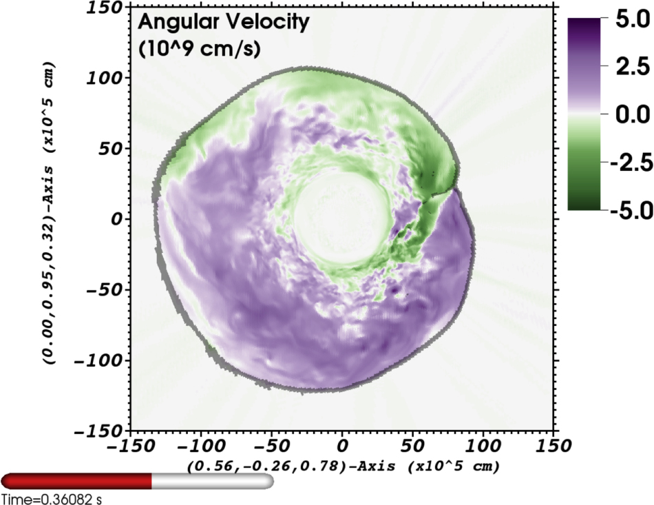
Figure 14. Gravitational wave spectrograms for simulations mesa20 (left) and mesa20_pert (right). For each time, the gravitational wave signal is multiplied by a Hanning window with a width of 50 ms. After the data is Fourier transformed, we calculate ![${\mathrm{log}}_{10}[| \tilde{{h}_{+}}{| }^{2}+| \tilde{{h}_{\times }}{| }^{2}]$](https://content.cld.iop.org/journals/0004-637X/865/2/81/revision1/apjaadcf7ieqn76.gif) (where the signal are those seen by an observer on the equator) and normalize to the same global maximum (across both plots) to allow for a direct comparison.
(where the signal are those seen by an observer on the equator) and normalize to the same global maximum (across both plots) to allow for a direct comparison.
Download figure:
Standard image High-resolution image
In addition to the bursts of GWs around 200 ms due to the imposed progenitor perturbations, we also see bursts of GW emission associated with the collapse of spiral SASI waves. In particular, the increased emission at ∼360 ms in mesa20 and at ∼400 ms in mesa20_pert. While not shown, we see a similar feature in mesa20_LR at ∼370 ms. The emission is concentrated at the peak PNS frequency, but does contribute power to other frequencies as well. In terms of the dynamics, both the accretion of progenitor perturbations and the collapsing spiral SASI waves are very similar. They both excite turbulence in the gain region marked by an increase in the lateral kinetic energy (see Figure 1).
Finally, we compare mesa20_LR and mesa20_v_LR. During the first ∼300 ms we see broad agreement in the GW signal between these two simulations. Starting at ∼350 ms, coincident with the increased SASI activity, the power in the GW signal of mesa20_LR grows while mesa20_v_LR stays roughly constant. This is in agreement with our previous observations, which show reduced SASI motions in the mesa20_v_LR simulation due to the larger shock radius and slower recession of the PNS core (see Figure 4).
4. Discussion and Conclusions
In this study, we have presented the first suite of 3D simulations using the FLASH hydrodynamics framework with energy-dependent, multidimensional, M1 neutrino transport. We perform eight 3D simulations exploring the impact of imposed progenitor perturbations, resolution, octant symmetries, dimensionality, and velocity dependence in the transport equations. For these simulations we use the same progenitor with a ZAMS mass of 20 M⊙ produced using the MESA stellar evolution package. We find no explosions in any of our 3D simulations.
We have presented a thorough analysis of each of the above-mentioned variations. The impact of imposed progenitor perturbations is clear. We find that the velocity perturbations we place in the silicon shell, particularly those located near the top of the shell, are very efficient at seeding turbulence in the post-shock flow. We find an enhancement of the lateral kinetic energy when these perturbations accrete through the shock, a corresponding increase in the neutrino heating, shock radius, and a quantitive measure of how close the simulation is to explosion. Ultimately we aspire to use progenitors evolved in full 3D (for as long as possible before collapse) in order to get a more physical set of initial conditions. We expect (following Couch & Ott 2015; Müller et al. 2017, and as we see here) that these precollapse asphericity are crucial in helping an explosion develop. Lower resolution, which leads to larger numerical seeds, slightly raises the level of turbulence as well and gives a slightly larger shock radius, and a higher measure of the closeness to explosion, however, this effect is smaller than that observed from the imposed perturbations. Overall, the low-resolution simulations behave qualitatively similar to the higher resolution simulations. Imposing octant symmetry places restrictions on the development of global instabilities, particularly the SASI. It is these lowest order modes that can play an important role in helping to support the shock at larger radii, which can increase the neutrino heating. These simulations, which lack these low-order modes are quantitatively further from explosion. We have explored, though a limited number of simulations, the impact of improved neutrino transport methods. The largest difference of these simulations, compared to the simulations performed without these improvements, is the presence of stronger PNS convection. The effect is a larger shock radius (by 30% at 300 ms), increased lateral kinetic energy, and an increased heavy-lepton neutrino luminosity. We discuss additional differences below.
We also explore in detail the SASI. We observe this phenomenon in all of our simulations without velocity dependence. We mainly observe spiral SASI modes, although there are nonzero, nonspiral components as well. Coincident with the SASI modes are correlated variations in the neutrino signals, showing at most a ∼5% variation on top of the baseline signal. In many cases, the spiral SASI modes buildup, become nonlinear, and collapse. This triggers a burst of turbulence that increases the neutrino heating and helps support and push the supernova shock to larger radii. None of these events leads to a successful explosion, however, each of these events temporarily brings the core-collapse event quantitatively closer to explosion. We suggest that such SASI-driven explosions may be one way the supernova shock can be reenergized. In such an event, the spiral SASI wave will have imparted a nonzero angular momentum to the core, even for progenitors with little or no initial rotation. We find that the typical final neutron star spin period for the spiral SASI waves in our simulation is ∼1 s. This relatively slow period is in part due to the small shock radii at the times when we see strong SASI activity. This limits the amount of angular momentum that can be built-up in the spiral SASI wave. Bearing in mind that we have only performed one full 3D simulation with velocity dependence (and it was performed at our lower resolution), we suggest that a consequence of the increased PNS and shock radii in that simulation is a lack of the presence of the SASI. This will take further exploration with more full 3D models with the full neutrino transport and our standard resolution.
While the one full 3D simulation with velocity dependence does not exhibit SASI motions, it does show conclusive evidence for the LESA phenomena that was first reported in Tamborra et al. (2014). The work presented here is the first reported independent confirmation of the LESA and the first to demonstrate that LESA is not an artifact of the ray-by-ray method. In this simulation we find a substantial dipole component in the total electron lepton-number emission, which grows starting at ∼200 ms after bounce and reaches a maximum at ∼300–400 ms after bounce. This dipole is stable, yet migratory, in direction. It shows excellent alignment with a dipole of the electron fraction in the convective PNS core. We confirm many of the observations seen in Tamborra et al. (2014), including hemispheric excess of neutrino heating and a larger average shock radius in the direction anti-aligned with the lepton-number dipole direction, and a larger mass accretion rate onto the PNS in the hemisphere aligned with the lepton-number dipole direction. It still remains unclear the mechanism from which this instability is initially generated and sustained. We conclude that the reason for seeing this only in the one simulation performed with velocity dependence is not the explicit presence of this improvement in the neutrino transport, but rather the impact of the improvement on the strength of PNS convection in the core. A stronger PNS convection appears to be conducive to the appearance of the LESA.
We also investigate the GW signal from our simulations. We see a large impact of the imposed progenitor perturbations on the GW signal. At the time when we see the largest impact on the dynamics, when the outermost layers of the silicon shell accrete through the shock, we see a large enhancement of the GW signal, with an amplitude approximately four to five times greater than the signal from the unperturbed simulation. Most of the excess power is at frequencies that are associated with oscillations of the PNS. When the aforementioned spiral SASI waves undergo collapse, we also see bursts of GWs. These bursts are coincident with increased turbulent activity in the gain region.
In summary, our suite of simulations reveals a plethora of 3D dynamics that altogether play a role in CCSNe. We show, through several mechanisms, that increased turbulent activity, however it arises, can play a crucial role in the shock dynamics by providing additional pressure support, facility increased neutron heating, and quantitatively bring the system closer to the point of explosion. While we see no explosions in the work presented here, we are confident that that simulation framework we have developed and assessed in this article will be extremely useful for our future explorations of 3D simulations of CCSNe.
We thank Jérôme Guilet, Hans-Thomas Janka, Kuo-Chuan Pan, Luke Roberts, and Irene Tamborra for helpful discussions and Kuo-Chuan Pan for assistance with the volume renderings in Figure 2. Partial support for this work (E.O.) was provided by NASA through Hubble Fellowship grant number 51344.001-A awarded by the Space Telescope Science Institute, which is operated by the Association of Universities for Research in Astronomy, Inc., for NASA, under contract number NAS 5-26555. S.M.C. is supported by the U.S. Department of Energy, Office of Science, Office of Nuclear Physics, under award numbers DE-SC0015904 and DE-SC0017955 and the Chandra X-ray Observatory under grant number TM7-18005X. The software used in this work was in part developed by the DOE NNSA-ASC OASCR Flash Center at the University of Chicago. This research used computational resources at ALCF at ANL, which is supported by the Office of Science of the U.S. Department of Energy under contract no. DE-AC02-06CH11357. We particularly thank Adrian Pope at ALCF for assistance. Additional resources from TACC under NSF XSEDE allocation TG-PHY100033, and on the Zwicky cluster at Caltech, which is supported by the Sherman Fairchild Foundation and by NSF award PHY-0960291.
Software: FLASH (Fryxell et al. 2000; Dubey et al. 2009), GR1D (O'Connor & Ott 2010; O'Connor 2015), Matplotlib (Hunter et al. 2007), yt (Turk et al. 2010), HEALPix/healpy (Górski et al. 2005), MESA (Paxton et al. 2011, 2013, 2015, 2018), and VisIt (Childs et al. 2012).