


Abstract
We study the polarized radio emission from young Type Ia supernova remnants by means of three-dimensional numerical MHD simulations and the assumption of relativistic electron distribution related to magnetic field energy density. In our simulations, the turbulent component of background plasma is taken into account by introducing a 3D Kolmogorov-like power spectrum. The simulation results indicate (i) the different orientations of the interstellar magnetic field around SNRs and lines of sight could produce different polarized radio emission shells, (ii) the fraction of polarization may be decreased through integrating the synchrotron emissivities along the line of sight, which is mainly due to the emission from the strong turbulent and disordered region of the magnetic field, and (iii) the total intensity is strong in some regions where the polarization degree is low.
Export citation and abstract BibTeX RIS
1. Introduction
The essential information on the degree of order and orientation of the magnetic field in the SNRs could be inferred by radio polarization observations, which is also a useful tool to diagnose the configurations of interstellar magnetic field (ISMF) and the small-scale component of turbulent plasma background around SNRs. The observed degree of polarization in SNRs is considerably lower than the maximal theoretical value, which reveals that the local magnetic field may contain a turbulent component.
Magnetic field plays a vital role in collisionless astrophysical shocks as well as acceleration of charged particles (Malkov & O'C Drury 2001). It can be amplified by cosmic-ray-induced streaming instability in the presence of efficient particle acceleration (Bell 2004; Riquelme & Spitkovsky 2009; Inoue et al. 2013) or by turbulent motions in the shock downstream in a turbulent medium (Giacalone & Jokipii 2007). The latter has been explored recently by Guo et al. (2012) and their results also indicate that the magnetic field is disordered significantly when SNRs evolve in the turbulent plasma medium.
The great diversity of emission morphology observed in SNRs, reflects not only different properties of the progenitors and explosion mechanisms, but also the properties of the ambient magnetic field and the matter distribution in the circumstellar and interstellar medium. A nonuniform medium has been introduced to explain the detected asymmetries of emission characteristics of SNRs through analytical methods (Hnatyk & Petruk 1999) or numerical simulations (e.g., Orlando et al. 2007; Fang et al. 2014; Yang et al. 2015; Petruk et al. 2018; Wang et al. 2018). Balsara et al. (2001) have performed three-dimensional magnetohydrodynamic simulations of an adiabatic SNR's evolution in both a uniform and turbulent interstellar medium. Their results indicate that a uniform medium could give rise to a bilateral radiation morphology. However, for the turbulent medium, the resulting synchrotron shell is very patchy and shows large variability in intensity. They have also calculated the polarization of the synchrotron emission and found that the most high fractional polarization region is spatially coincident with the region with strong intensity. The emission morphologies of some SNRs are obtained by specific configurations of the surrounding ISMF and interstellar medium, in order to be comparable with the observational results (e.g., Schneiter et al. 2010; Bocchino et al. 2011; Schneiter et al. 2015; Velázquez et al. 2017). Bandiera & Petruk (2016) present a detailed but numerically lighter treatment of radio synchrotron emission for shell-type SNRs. The configurations there allow the authors to investigate several effects related with magnetic field and polarization, and to synthesize the emission and polarization maps for shell-like SNRs with different specific conditions. For a uniform magnetic field, a high polarization degree is obtained when this magnetic field is parallel to the line of sight or if it is on the sky plane. However, when an isotropic random magnetic field component combines with an ordered magnetic field component oriented vertically to the line of sight, a low polarization degree is obtained. The numerical simulation results also imply that the radial magnetic field could be produced in the Rayleigh–Taylor instability region or in those places where the shock-compression magnetic field amplified due to shock penetrating into a clumpy medium (Jun & Norman 1996). Radio polarization observations have shown that many young SNRs possess a predominantly radial magnetic field structure, which is mainly due to magnetic field amplification along the R–T fingers (Milne 1987). One popular case is SN 1006(G327.6+14.6). Considering its high Galactic latitude and bilateral symmetric morphology, SN 1006 is an ideal target for the study of radio polarization and surrounding ISMF distribution (Kundu 1970; Dickel & Milne 1976; Reynolds & Gilmore 1993). SN 1006 is a typical bilateral Type Ia SNR with two bright limbs perpendicular to the Galactic plane based on the detected morphologies from radio to γ-ray (see Katsuda 2017 for a recent review). Recent radio polarization observations for SN 1006 have revealed that the polarization fraction is lower (∼0.17) in the two bright radio and X-ray lobes (NE and SW sectors) compared with the faint limbs (located in SE and NW sectors with a polarization fraction ∼0.7; Reynoso et al. 2013). This result can be interpreted as evidence of a turbulent magnetic field in the bright lobes, while there is a highly aligned field in the faint areas. Despite of the polarization results, most of its shell appears to own a radial magnetic field distribution and a subsequent detailed analysis on polar-referenced distribution points to an ambient magnetic field roughly parallel to the Galactic plane.
The main goal of this paper is to study the radio polarized emission from young Type Ia supernova remnants and clarify the effects on the polarized emission morphologies exerted by different configurations of the ISMF orientations and lines of sight. For this purpose, we implement 3D MHD simulations based on the assumption that relativistic electron spatial distribution is closely related to the distribution of magnetic field energy density (Yang & Liu 2013). At the same time, the relativistic electron spectrum possess a power-law shape with exponential cutoff, which is inferred from the multiband data fittings. In order to produce the polarized radio emission morphologies, we introduce the Stokes parameters and use their local spectral densities to obtain the intensity.
The structure of this paper is as follows. A detailed description of our model and initial setup of simulations are described in Section 2. The method for producing the synthetic radio polarized emission maps is introduced in Section 3. The simulation results are presented in Section 4, while some discussion and conclusions are given in Section 5.
2. Model Description
The numerical simulations are carried out with the paralleled 3D MHD code PLUTO (Mignone et al. 2007, 2012). This code provides various hydrodynamic modules and algorithms for solving the full sets of ideal MHD equations with different geometry systems. In our simulations, Cartesian geometry (x1, x2, x3) and a computational cube of 24 pc in each direction are chosen for a uniform grid distribution (512 × 512 × 512), corresponding to a resolution of 0.046 pc.
For young Type Ia SNRs, the simulating parameters setup is described as follows, a supernovae explosion (E0 = 2 × 1051 erg) is injected into Galactic space with an initial radius R0 = 0.5 pc, which is located at the center of the computational domain (for SNe Ia, see a recent review by Wang 2018). The initial ejecta profile includes two parts, that is, a uniform density (ρc) within a radius rc containing 4/7 of the total mass (Mejecta = 1.4 M⊙) in the inner part and a distribution of power law ρ ∝ r−7 in the outer part. The velocity of material in ejecta has a linear profile with r expanding freely to a uniform circumstellar medium. The rc and ρc are calculated by using Equations (1)–(3) of Jun & Norman (1996). The age of the benchmark SNR is set to be about 1000 years, which is also the end time of our simulations.
In the simulations, the benchmark SNR evolves into a turbulent background plasma, and the fluctuations of both the magnetic field and the density have a 3D Kolmogorov-like power spectrum, which is consistent with the observations of interstellar turbulence. The detailed descriptions of the fluctuations both in magnetic field and density are given by Giacalone & Jokipii (2007), and we give a brief summary below.
The magnetic field includes a uniform large-scale component (B0 = 3 μG), and a turbulent component δB(x1, x2, x3). The background magnetic field, sum of the two components, is then B(x1, x2, x3) = B0 + δB(x1, x2, x3). The fluctuations of the density, a lognormal probability is adopted with  , where δf owns the form of a 3D Kolmogorov-like power spectrum with a wave variance
  , and n0 = 0.05 cm−3 is the average number density of the surrounding ISM. In this study, the fluctuating component of the magnetic field is taken to be δB = 0.2B.
3. Synthetic Total and Polarized Radio Emission Maps
The relativistic electrons producing the nonthermal multiband emission are accelerated by supernova remnant shocks, and the electron spatial distribution satisfies a power-law form, i.e., N(E) ∼ E−s. To simulate the nonthermal radiative characteristics of SNRs via using MHD methods, Yang & Liu (2013) have derived energy equipartition between energetic electrons and magnetic field energy, and the corresponding electron spectrum is given by

where s = is the spectrum index of the power law deduced from the radio observations, and Ecut is the cutoff energy. In the following simulation, s = 2.2 and Ecut = ∼20 TeV are adopted (Allen et al. 2008; Green 2009) and we assume that the relativistic electron distribution considered here is isotropic. To construct maps of polarized radio emission, it is convenient to use the local densities of the Stokes parameters ( ). We can integrate these quantities along the line of sight weighted with the distribution function of energetic electrons (i.e., Equation (1)).
For an individual electron with energy E, the flux densities of polarization radiated in two principal directions are  and
and  , as given by Ginzburg & Syrovatskii (1965; their Equation 2.20). θB is the angle between the local magnetic field B(x1, x2, x3) and the direction to the observer, then the local spectral densities of the Stokes parameters are given through
  and
and  :
:
where the angle χ defines the position of the major axis of polarization ellipse and lies in the plane perpendicular to the observer direction, and  is the ratio of principal axes of the oscillation ellipse.
In order to produce the images of polarized radio emission, we assume that the line of sight is along xi, where the index i is either x1, x2, or x3. So we can integrate the local spectral densities of the Stokes parameters along the xi direction weighted with electron distribution to acquire the intensity:

where Si(ν) are Stokes parameters integrating along the line of sight xi. Si(ν) represent the polarization state of an electromagnetic wave propagating through space and contain four parameters (I, Q, U, V ), which are the total intensities weighted with the relativistic electron group. The fourth Stokes parameter V is zero here due to an isotropic electron velocity distribution. The degree of linear polarization is determined in a standard way as  and
and  . The Stokes parameters turn out to be an important tool to compare numerical models with radio polarization observations and contribute to the determination of ISMF configuration (Reynoso et al. 2013; Velázquez et al. 2017).
4. Numerical Results
We used the previously described numerical methods to study the polarized radio emission from young Type Ia supernova remnants based on different ISMF orientations and the lines of sight (to the observer). In this section, we will display our simulation results, which are under the assumption that the synthetic polarized radio emission is at 1.4 GHz.
For the synthetic polarized radio emission maps, to investigate the effects exerted by different orientations of ISMF around SNRs and lines of sight, we consider three different scenarios: (1) The orientation of the large-scale magnetic field is parallel with the line of sight (for example, the line of sight is along x3 and the orientation of the large-scale magnetic field is also along x3). (2) The orientation of the large-scale magnetic field is vertical to the line of sight (for example, the line of sight is along x1, while the orientation of the large-scale magnetic field is parallel with  plane. The inclined angle between the magnetic field and the x3-axis is 30°). (3) The same configuration with scenario (2) except that the line of sight is along x2.
The simulation results of scenario (1) are shown in Figure 1. As for the profiles of the Stoke parameters panels (a) log I, (b) log  , and (c) log
  , the typical shell-like emission profile is produced, and the local emission intensity is enlarged due to the remnant evolving in the turbulent plasma background, which also induces the production of thin filament structure. The synthetic polarized emission maps apparently exhibit shell-bright structure, resembling the observational results of some SNRs. In this case, the polarization degree or fractional polarization map (i.e., panel (d)) appears to exhibit a strong linear polarization approaching the theoretical maximum value, indicating that the regular component of the magnetic field dominates over other components inside the remnant (along the line of sight). In panel (f), we plot the distribution of the polar-referenced angle (the angle between the magnetic field orientation and the local radial direction) and it is clear to see that the radial magnetic field orientation is overwhelming inside the whole remnant. While most of the shell seems to have a radial magnetic field distribution, there are still some departures existing. Comparing panel (f) with panel (d), there seems to be no evident spatial correlation between magnetic field orientation and fractional polarization distribution.

Figure 1. Simulation results of scenario (1) are displayed. Panels from (a) to (f) are the maps of (a) log I; (b)  (c)
(c)  (d) polarization degree; (e) polarization angle; and (f) the polar-referenced angle, respectively. Specifically, the polar-referenced angle is the angle between the magnetic field orientation and the local radial direction.
Download figure:
Standard image High-resolution imageThe above result is further confirmed in Figure 2, where panels (a) and (c) display the statistical histograms of the polar-referenced angle distribution from 0 to 10 pc, while panels (b) and (d) only contain the contribution mostly from the outer shell (7–10 pc). Specifically, for panels (c) and (d), we only consider those grid points whose emission intensity is larger than 10% of the maximum value of I. All panels in Figure 2 clarify that the distribution of the polar-referenced angle is concentrated at about 0°. Panel (a) shows the counts with radius between 0 and 10 pc, while panel (b) accounts for only 7–10 pc, and the peak value in panel (b) is lower than that in (a) by a factor of 3. However, the peak value in panel (d) is lower than that in (c) only by a factor of 1.2. The difference is due to the fact that we consider those grid points whose emission intensity is larger than 10% of the maximum value of I in panels (c) and (d). As most of the grid points meeting our requirement (larger than 10% of the maximum value of I) are in the region between 7 and 10 pc (see panel (a) in Figure 1), the corresponding statistical histograms of the two regions (0–10 pc and 7–10 pc) should be roughly equivalent.
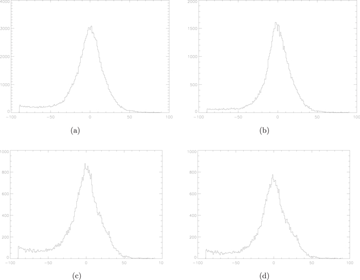
Figure 2. Distribution of the polar-referenced angle extracted from panel (f) in Figure 1. Panels (a) and (c) show the counts with radius between 0 and 10 pc in all directions. Panels (b) and (d) show the counts with radius between 7 and 10 pc in all directions. Here, for panels (c) and (d), we only consider those grid points whose emission intensity is larger than 10% of the maximum value of I.
Download figure:
Standard image High-resolution imagePanel (e) in Figure 1 shows the polarization angle distribution, which we define as the angle of the electric field orientation with respect to the positive x axis for the upper half (the negative x axis for the bottom half). The polarization angle is counted counterclockwise and it keeps a positive value for both halves (0°–180°). As the electric field orientation is perpendicular to the magnetic field orientation on the sky plane, the polarization angle distribution can be considered to be supplementary to the polar-referenced angle distribution map (i.e., panel(f)). If the orientation of the projected magnetic field is primarily radial around the whole SNR shell, then the resulting polarization angle distribution map should be roughly uniformly distributed between 0° and 180° for left half and right half respectively. Combining panel (e) with panel (f), it is clear to see that the radial orientation is predominant.
In Figure 3, we give the simulation results of scenario (2). As shown in panels (a)–(c), one can see the bilateral or broken shell-like radiation morphology. The total intensity image in panel (a) exhibits one distinctive region: the inner turbulent shell. This bright clumpy inner shell is clearly seen in the plot, which is probably the consequence of the amplified magnetic field triggered by Rayleigh–Taylor instability. The clumpy inner shell includes many small-scale turbulent structures, and one can find plumes with strong intensity inside this turbulent region, where there are strong fluctuations of magnetic field and matter density in the plasma background. However, the total intensity in periphery of the SNR shell is fainter compared to the inner region. Maybe in young Type Ia SNRs, such an inner bright shell appears to be the main visible shell in radio band if local conditions are consistent with the configuration of scenario (2). The linear polarization degree distribution in panel (d) clearly shows a low fractional polarization inside the remnant, which is quite different from the polarization degree distribution of scenario (1) (i.e., Figure 1 panel (d)) and is mainly due to the turbulent magnetic fields dominating over this region (along the line of sight). However, the bright bilateral arcs where the total intensity is strong has a relatively high fractional polarization compared with the other region inside the remnant.

Figure 3. Simulation results of scenario (2) are displayed. Panels from (a) to (f) are the maps of (a) log I; (b)  (c)
(c)  (d) polarization degree; (e) polarization angle; and (f) the polar-referenced angle, respectively. Specifically, the polar-referenced angle is the angle between the magnetic field orientation and the local radial direction.
Download figure:
Standard image High-resolution imageIn panel (f), the polar-referenced angle distribution is shown. It is obvious to see that the radial magnetic field orientation is no longer overwhelming inside the remnant and the tangential component increases. The polar-referenced angle distribution is more unambiguous in Figure 4, where panels (a) and (c) display the distribution of the polar-referenced angle from 0 to 10 pc, while panels (b) and (d) only contain the contribution originating mostly from the outer shell (7–10 pc). Specifically, for panels (c) and (d), we only consider those grid points whose emission intensity is larger than 10% of the maximum value of I. All panels in Figure 4 clarify that the distribution of the polar-referenced angle is concentrated at about −80°, but not as prominently because other components are comparable. However, it should be mentioned that the two extreme angles (i.e., 90° and −90°) actually represent the same orientation (tangential). Panel (b) in Figure 4 displays the the distribution originating mostly from the outer shell (7–10 pc) and the tangential orientation seems predominant. For panels (c) and (d) in Figure 4, where we only consider those grid points whose emission intensity is larger than 10% of the maximum value of I, the results are similar to panels (a) and (b). Panel (e) displays the polarization angle distribution, which we have already described previously. Combining panel (e) with panel (f), it is obvious that the orientation of the projected magnetic field in the outer shell is similar with the orientation of the large-scale component, indicating that the SNR may retain some knowledge of the background magnetic field even after passage of the shock front (Reynoso et al. 2013).

Figure 4. Distribution of the polar-referenced angle extracted from panel (f) in Figure 3. Panels (a) and (c) show the counts with radius between 0 and 10 pc in all directions. Panels (b) and (d) show the counts with radius between 7 and 10 pc in all directions. Here, for panels (c) and (d), we only consider those grid points whose emission intensity is larger than 10% of the maximum value of I.
Download figure:
Standard image High-resolution imageThe only difference between scenarios (2) and (3) is the orientation of the line of sight. For scenario (3), the line of sight is along the x2 axis, while for scenario (2) the line of sight is along the x1 axis (the orientation of the large-scale magnetic field is parallel with the  plane in scenarios (2) and (3)). Figure 5 displays the simulation results of scenario (3). From panels (a)–(c), one can see similar shell-like radiation morphology to that in Figure 1. Though the synthetic maps here are similar to those in Figure 1 on the whole, the specific morphologies are different.

Figure 5. Simulation results of scenario (3) are displayed. Panels from (a) to (f) are the maps of (a) log I; (b)  (c)
(c)  (d) polarization degree; (e) polarization angle; and (f) the polar-referenced angle, respectively. Specifically, the polar-referenced angle is the angle between the magnetic field orientation and the local radial direction.
Download figure:
Standard image High-resolution imagePanel (d) in Figure 5 shows the linear polarization degree of the whole remnant. The fractional polarization is low inside the remnant with two distinct regions on both sides. In our simulations, the fluctuated and disordered ambient fields have been introduced to decrease the polarized emission, which resemble the actual astrophysical environments. Since the large-scale magnetic field in this case has a component along the x2-axis (parallel with the line of sight), the average fractional polarization inside the remnant is a little higher than that of scenario (2) (see Figure 3 panel (d)). By comparing panel (a) with (d), an interesting result is obtained: in some regions of the periphery, the total intensity is strong while the fractional polarization is low. The result here is somewhat conflicting with the results of scenarios (1) and (2). In Figures 1 and 3, by comparing panels (a) with (d), we may conclude that most of the high fractional polarization region is spatially coincident with the region with strong total intensity. The result obtained here is mainly caused by the different orientation of ISMF and line of sight with scenario (3).
The polar-referenced angle distribution and its statistical histograms are shown in Figure 5 panel (f) and Figure 6 respectively. In panel (f), it is clear to see that the radial orientation dominates over the outer shell while the orientation is predominantly quasi-tangential in the inner shell. A detailed analysis is given by Figure 6. In Figure 6 panel (a), the polar-referenced angle distribution peaks at about 0° but not so prominent compared with Figure 2 panel (a), indicating that inside the remnant there is a reduction in the radial magnetic field orientation component. However, as shown in Figure 6 panel (b), the distribution still peaks at about 0° and its shape is similar to that in Figure 2 panel (b), which in turn implies that the reduction of the radial magnetic field orientation component mostly takes place in the inner shell. For panels (c) and (d), where we only consider those grid points whose emission intensity is larger than 10% of the maximum value of I, the statistical histograms show clearly radial orientation dominance. The result here is similar to that in Figure 2 panels (c) and (d), which indicate that most of the grids points meet our requirement (larger than 10% of the maximum value of I) are in the region between 7 and 10 pc (see Figure 5 panel (a)).
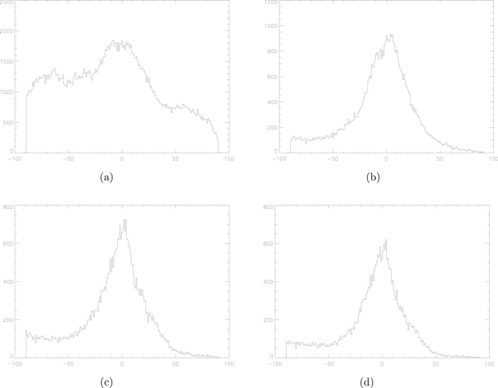
Figure 6. Distribution of the polar-referenced angle extracted from panel (f) in Figure 5. Panels (a) and (c) show the counts with radius between 0 and 10 pc in all directions. Panels (b) and (d) show the counts with radius between 7 and 10 pc in all directions. Here, for panels (c) and (d), we only consider those grid points whose emission intensity is larger than 10% of the maximum value of I.
Download figure:
Standard image High-resolution imageOur synthetic intensity maps here are acquired by integrating the local spectral densities of the Stokes parameters along the line of sight weighted with electron distribution, based on the assumptions of turbulent background and energy equipartition between energetic electrons and magnetic field energy (the corresponding electron spectrum is proportional to B2; Yang & Liu 2013). As a result, the synthetic maps show variations in intensity with orders of magnitude that can be seen clearly in Figures 1, 3, and 5. However, the polarization observations usually exhibit at most 1.5 orders of magnitude for the intensity maps, and are thus shown in linear scale (Reynoso et al. 2013, 2018; Zanardo et al. 2018). In order to make comparisons with observations easier, we have made an attempt to display the previous intensity maps in linear scale. In Figures 7–9, we display the synthetic intensity maps of scenarios (1)–(3) in linear scale. In order to provide a proper display in linear scale, we have scaled our maximum value, and cells with intensities larger than the maximum value are displayed in white. As can be seen from the figures, the maps here show radiation morphologies that are similar to previous results shown in logarithmic scale.
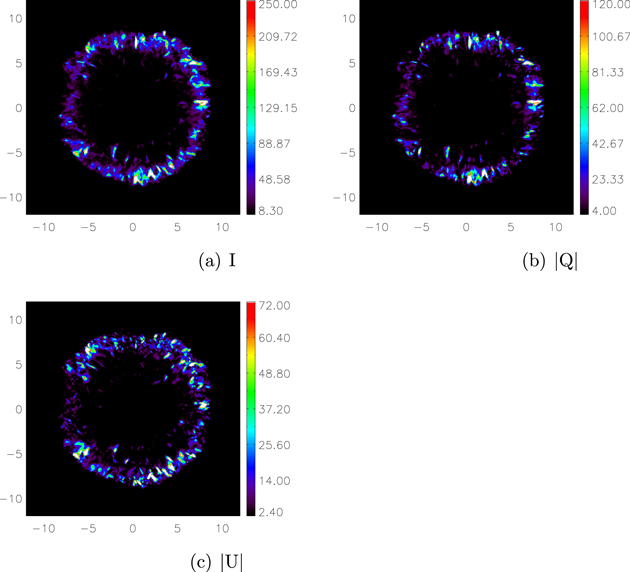
Figure 7. Synthetic intensity maps of scenario (1) are displayed in linear scale. For a proper display, we have scaled our maximum value, and cells with intensities larger than the maximum value are displayed in white. All of the values shown in the color bar are in units of 10−7.
Download figure:
Standard image High-resolution image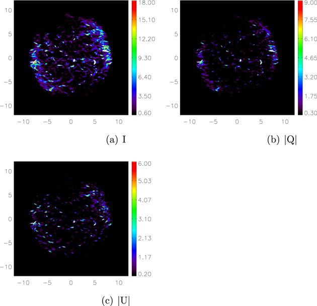
Figure 8. Synthetic intensity maps of scenario (2) are displayed in linear scale. For a proper display, we have scaled our maximum value, and cells with intensities larger than the maximum value are displayed in white. All the values shown in the color bar are in units of 10−8.
Download figure:
Standard image High-resolution image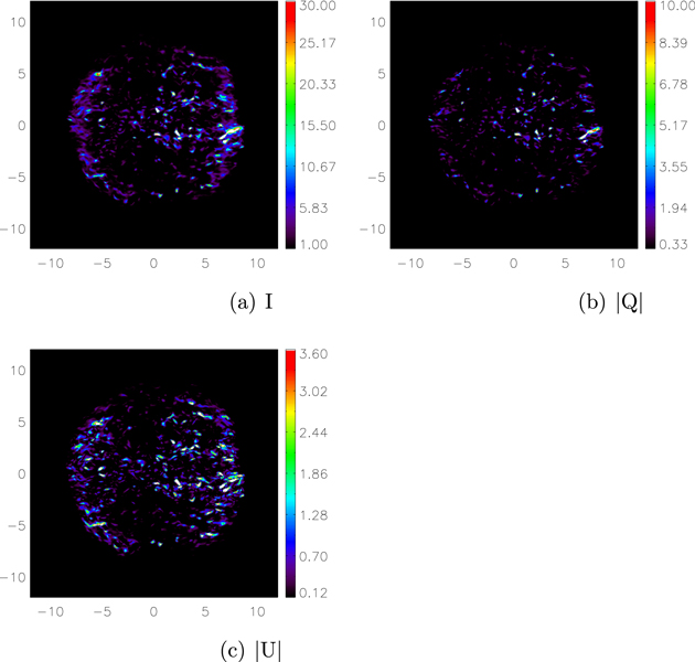
Figure 9. Synthetic intensity maps of scenario (3) are displayed in linear scale. For a proper display, we have scaled our maximum value, and cells with intensities larger than the maximum value are displayed in white. All the values shown in the color bar are in units of 10−8.
Download figure:
Standard image High-resolution image
5. Summary and Discussion
A study on the polarized radio emission from young Type Ia supernova remnants has been performed by means of three-dimensional numerical MHD simulations and assuming that the distribution of relativistic electrons is closely related to the magnetic field energy density (Yang & Liu 2013).
We have considered three different scenarios with respect to the ISMF orientations around SNRs as well as lines of sight, and made an attempt to clarify the effects on the synthetic polarized emission maps exerted by these scenarios. For our purpose, the three-dimensional numerical MHD simulation is a realistic choice as only a three-dimensional model can account for a magnetic field that is tilted with the line of sight (Schneiter et al. 2015). The perturbations both in magnetic field and density are supported by abundant observations and have been introduced to explain the detected asymmetries of SNR emission characteristics by many authors. Here we considered the fluctuations both in magnetic field and density with the 3D Kolmogorov-like power spectrum given by Giacalone & Jokipii (2007).
Our simulation results of scenarios (1)–(3) are shown in Figures 1–6. We synthesized maps of the polarized emission that included Stokes parameters I, Q, and U, and acquired the distributions of polarization degree, polarization angle, and polar-referenced angle. The resulting polarized intensity maps are quite different from each other (see panels (a)–(c)), indicating that different orientations of ISMF and lines of sight could produce different polarized radio emission morphologies.
In scenario (1), the ISMF orientation is parallel to the line of sight. So the fractional polarization (panel (d)) is high in such a case because the synchrotron emissivities are integrated along the line of sight where the ISMF dominates. However, in scenarios (2) and (3), the orientations of the ISMF are not parallel with the line of sight. In such cases, the fractional polarization is reduced via integrating the synchrotron emissivities along the line of sight where the turbulent component dominates. Despite the different configurations for setting up, our results here are comparable with partial results obtained in Bandiera & Petruk (2016). Moreover, in scenarios (1) and (2), most high fractional polarization regions are spatially coincident with the region of strong total intensity (see also Balsara et al. 2001). While in scenario (3), some regions on the periphery exhibit strong total intensity with low fractional polarization.
By acquiring the distributions of polarization angle and polar-referenced angle, we determined the orientation of the projected magnetic field inside the whole SNR in each scenario. In scenario (1), most of the SNR shell seems to have a radial magnetic field distribution. However, when the orientations of the ISMF and lines of sight changed, the resulting distribution deviated far from radial orientation, indicating that the SNR may retain some knowledge of the ambient field even after passage of the forward shock (see panels (e) and (f) in each scenario's simulation results).
In summary, our simulation results on the synthetic total and polarized radio emission maps provide us with evidence that different orientations of ISMF around SNRs and lines of sight could produce different polarized emission maps. The resulting polarization degree map and the magnetic field orientation distribution inside the remnant are also affected.
We thank the anonymous referee for very constructive comments. We gratefully acknowledge the computing time granted by the Yunnan Observatories and provided on the facilities at the Yunnan Observatories Supercomputing Platform. This work is mainly supported by the National Science Foundation of China 11673060, and the Natural Science Foundation of Yunnan Province under grant 2016FB003. L.Z. is partially supported by the Natural Science Foundation of China (NSFC; NSFC 11433004 and U 1738211).