


Abstract
The standard model of flares predicts the existence of a fast-mode magnetohydrodynamic shock above the looptops, also known as termination shock (TS), as the result of the downward-directed outflow reconnection jets colliding with the closed magnetic loops. A crucial spectral signature of a TS is the presence of large Doppler shifts in the spectra of high-temperature lines (≥10 MK), which has been rarely observed so far. Using high-resolution observations of the Fe xxi line with the Interface Region Imaging Spectrograph (IRIS), we detect large redshifts (≈200 km s−1) at the top of the bright looptop arcade of the X1-class flare on 2014 March 29. In some cases, the redshifts are accompanied by faint simultaneous Fe xxi blueshifts of about −250 km s−1. The values of red and blueshifts are in agreement with recent modeling of Fe xxi spectra downflow of the reconnection site and previous spectroscopic observations with higher temperature lines. The locations where we observe the Fe xxi shifts are co-spatial with 30–70 keV hard X-ray sources detected by the Reuven Ramaty High Energy Solar Spectroscopic Imager (RHESSI), indicating that nonthermal electrons are located above the flare loops. We speculate that our results are consistent with the presence of a TS in flare reconnection models.
Export citation and abstract BibTeX RIS
1. Introduction
Flares are the most powerful events in the solar atmosphere, and they are often accompanied by the ejection of coronal material and energetic particles into space, severely affecting the space weather. Even though the details of the current models of flares are highly debated, these energetic events are commonly thought to be caused by magnetic reconnection in the corona and the associated magnetic energy release. The standard reconnection-based model of flares (CSHKP; Carmichael 1964; Sturrock 1968; Hirayama 1974; Kopp & Pneuman 1976) is supported by a number of observations, including those of cusp-like structures visible in the soft X-rays (e.g., Tsuneta et al. 1992); hard X-ray (HXR) sources above the flare loop (Masuda et al. 1994); reconnection outflows and inflows (e.g., Yokoyama et al. 2001; Liu et al. 2013); field-line shrinkage (Forbes & Acton 1996; Reeves et al. 2008); and chromospheric evaporation from the flare footpoints (e.g., Li et al. 2015; Polito et al. 2015, 2016, 2017; Dudík et al. 2016). One of the predictions of this model is the presence of fast-mode magnetohydrodynamics (MHD) shocks, also referred to as termination shocks (TS), which are created by the downward-directed reconnection jets colliding with the reconnected loops (e.g., Forbes 1986; Yokoyama & Shibata 1998). Strong evidence for both the existence of TS and its crucial role in particle acceleration has been provided by recent radio and HXR observations (e.g., Aurass & Mann 2004; Mann et al. 2009; Chen et al. 2015). Of particular importance is the work of Chen et al. (2015), who observed several radio spikes during a C-class flare with the Karl G. Jansky Very Large Array. The morphology of the spikes was consistent with those of a TS, and they were located slightly above a coronal HXR source observed by the Reuven Ramaty High Energy Solar Spectroscopic Imager (RHESSI; Lin et al. 2002), as predicted by numerical simulations (e.g., Yokoyama & Shibata 1998; Takasao et al. 2015).
Flare reconnection models also suggest the presence of a deflection sheath formed immediately downstream of the shock, where the flow is diverted around the closed loops (e.g., Forbes 1986; see also Figure 1). The deflected flows should be observed as oppositely directed flows of high-temperature plasma, which would be visible by the spectroscopic instruments as blue/redshifts, depending on the inclination of the loops (see Figure 1). Direct observations of the flows in both up and downstream of the shock are difficult to obtain and extremely rare, as they are complicated by the low density of the plasma in those regions, as well as the limited spatial and temporal resolution of the instruments. In the case of oblique flares (located between the solar limb and disk), the deflected flows due to the TS could also be confused with the reconnection outflows, and a careful analysis of the loop geometry is necessary. It should be noted that the reconnection outflow region might be fainter and harder to observe than the flow in the downstream region because of the lower density of the upstream plasma, which is also more likely to be out of ionization equilibrium (Imada et al. 2011). On the other hand, downstream of the shock, the density is increased by around a factor of two (Forbes 1986), resulting in a higher emission measure of the plasma and a faster ionization timescale.
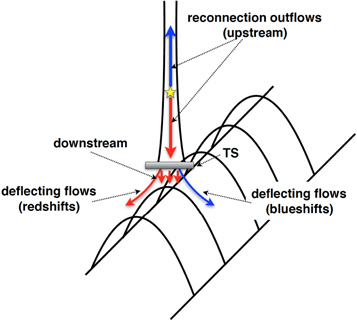
Figure 1. Cartoon illustrating the standard picture of termination shocks (TS) in flares. TS are created when the reconnecting outflow jets collide with the closed loops. The flows that are defected from the shock region around the closed loops (deflecting flows) can be visible as blue and/or redshifts in the spectra of high-temperature lines, depending on the orientation of the flare loops.
Download figure:
Standard image High-resolution imageHigh-velocity (800–1000 km s−1) flows in the Fe xxi 1354.08 Å line (≈10 MK) at the top of the loops arcade were first observed with the Solar Ultraviolet Measurements of Emitted Radiation (SUMER; Wilhelm et al. 1995) by Innes et al. (2003). More recently, Wang et al. (2007) found blue and redshifts (≈400 km s−1) in the Fe xix (≈8 MK) line with SUMER, which were interpreted by the authors as the reconnection outflows predicted by the flare reconnection models. Both observations were performed with a single-slit position for the spectrometer, and therefore lacked good spatial coverage. The first high-resolution spectral scannings of fast hot flows were then obtained with the Hinode/EUV Imaging Spectrometer (EIS; Culhane et al. 2007) in the Fe xxiii–Fe xxiv high-temperature lines, formed at about 10–20 MK during flares. Hara et al. (2011) found strong blueshifts (≈200 km s−1, suggestive of reconnection outflows), as well as smaller redshifts (≈30 km s−1, possibly produced downstream of the fast-mode shock), in the EIS flare lines during a small B9.5 class flare. Further, Imada et al. (2013) observed blueshifts and redshifts of at least 400 km s−1 in the Fe xxiv spectra, which they interpreted as the hot flows in the downstream of the fast-mode shocks, also supported by the analysis of high-resolution images by the Atmospheric Imaging Assembly (AIA; Lemen et al. 2012) on board the Solar Dynamics Observatory (SDO; Pesnell et al. 2012).
Since 2013, the Interface Region Imaging Spectrograph (IRIS; De Pontieu et al. 2014) has provided the observation of the Fe xxi line at 1354.08 Å (formed in the high-temperature ≈10 MK plasma during flares), with unprecedented spatial (≈0 33), spectral (≈3 km s−1) and temporal resolution (up to 1–2 s), significantly improving (by a factor of 10 or more) on the spatial resolution of EIS and previous spectroscopic instruments. Tian et al. (2014) reported the first evidence of large redshifts (≈125 km s−1) in the IRIS Fe xxi line at the looptops of a C-class flare in 2014, which were interpreted as the downflow component of the reconnection outflows. Prompted by the observations presented by Tian et al. (2014), Guo et al. (2017) used different MHD models of flare reconnection to synthesize the spectra of the IRIS Fe xxi line in both up and downstream of the shock. In their models, the authors assumed either Petschek-type reconnection (Petschek 1964) or plasmoid instability reconnection, which produced very different synthetic Fe xxi profiles. In particular, the Petschek-type reconnection (Figure 4 of Guo et al. 2017) predicted a Fe xxi spectrum dominated by two line components centered around 700 km s−1 (associated with the reconnecting outflows), and one more intense redshifted component by around 250–300 km s−1 (associated with the flows downstream of the shock). Such a multicomponent profile was obtained for a disk flare, whereas in the case of a oblique flare, the deflected flows from the TS should also be visible as both blueshifts and redshifts.
In this work, we present the observation of Fe xxi line profiles showing either large redshifts (200 km s−1) or both redshifts and blueshifts (−250 km s−1) at the looptops of the 2014 March 29 X-class flare observed by IRIS. The shifts are co-spatial to HXR sources observed by RHESSI. We interpret these flows as a possible signature of a TS.
The paper is structured as follows. Section 2 describes the IRIS, AIA, and RHESSI observations, whereas Section 3 describes the analysis of the IRIS Fe xxi spectra. Finally, Section 5 discusses and summarizes our findings.
2. Observations
On 2014 March 29, a large X1.0-class flare occurred on the AR NOAA 12017 between 17:35 and 17:54 UT. This is a well-studied event that was simultaneously observed by several satellites, including IRIS, SDO, Hinode, and RHESSI (e.g., Aschwanden 2015; Battaglia et al. 2015; Kleint et al. 2015; Li et al. 2015; Young et al. 2015; Kowalski et al. 2017; Woods et al. 2017).
Figure 2 shows the soft X-ray light curves of the flare as observed by the GOES satellite in the 1–8 Å channel. The flare started at about 17:35 UT, had a rapid impulsive phase, and peaked at ≈17:48 UT. The soft X-ray flux then gradually decreased to its pre-flare value from about 19:30 UT, after a slow gradual phase. IRIS, Hinode/EIS, and RHESSI observed the whole impulsive and part of the gradual phase of the flare until about 17:54 UT, 18:00 UT and ≈18:15 UT, respectively, as indicated by the colored arrows in Figure 2. Some precursor activity was observed up to 40 minutes prior to the onset of the flare, in the form of large blueshifts and nonthermal broadening of several UV/EUV spectral lines observed by IRIS and EIS (Woods et al. 2017).
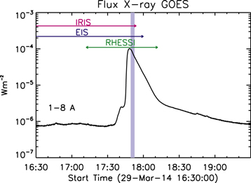
Figure 2. Soft X-ray light curves of the 2014 March 29 flare as observed by the GOES satellite in the 1–8 Å channel. The colored arrows indicate the duration of the IRIS, EIS, and RHESSI observations. The filled colored area indicates the period over which we observe the Fe xxi redshifts at the flare looptops.
Download figure:
Standard image High-resolution imageThe flare was likely to be triggered by the rearrangement of the magnetic field caused by a fast filament eruption that occurred at about 17:45 UT (Kleint et al. 2015). The eruption was closely followed by the rapid increase of the chromosphere ribbon emission as visible in the IRIS SJI images and, from around 17:46 UT, by strong evaporating flows in the high-temperature Fe xxi line observed by IRIS, which lasted until at least six minutes after the peak of the flare (Young et al. 2015). Bright loop emission was observed in the AIA 131 Å channel (mainly showing Fe xxi plasma during flares) from around 17:46 UT, just after the chromospheric evaporation from the ribbons was first detected. See the animation showing an overview of the flare and its evolution over time.
In this work, we focus on studying a faint redshifted Fe xxi emission visible at the top of the high-temperature loop arcade from around 17:49:21 UT until almost the end of the IRIS observation, which is indicated by the filled colored area in Figure 2. To study this emission, we analyzed data from IRIS, RHESSI, SDO/AIA, and Hinode/EIS, whose reduction is briefly described in Section 2.1.
2.1. Data Reduction
2.2. IRIS
IRIS observed the AR 12017 during 180 very large coarse eight-step rasters with a cadence of 75 s over the period 14:09 to 17:54 UT. Each raster step was separated by 2'', with a raster size of 14'' × 174'' and exposure time of 9 s. IRIS slit-jaw images were obtained alternatively in the Si iv 1400 Å, Mg ii h 2796 Å, and Mg ii wing 2832 Å filters with a cadence of 26, 19, and 75 s, respectively, over a field of view of 167'' × 174'' . The three SJI filters are dominated by plasma formed at around 104.9, 104, and 103.8 K, respectively. We used level 2 IRIS data, which are processed for dark current subtraction, flat-field, and geometry correction. In the level 2 data, the orbital wavelength calibration is automatically performed;4 however, we also performed a manual check of the calibration based on the measurement of the centroid of the O i 1355.568 Å photospheric line, which usually shows a small Doppler shift, of the order of 2–5 km s−1. We note that this uncertainty is very small compared with the average value of velocities we measure in this work (≈200 km s−1).
2.3. SDO
We also analyze images from the SDO/AIA telescope, which provide a context for the observed event in coronal and flare temperatures over a larger field of view, and the SDO/Helioseismic and Magnetic Imager (HMI; Scherrer et al. 2012), which provide information about the line-of-sight magnetic field. The full-Sun AIA and HMI level 1 data were converted to level 1.5 using the Solarsoft routine aia_prep, which performs the alignment between different filters and the adjustment of the telescope platescale, and remaps the HMI data into the AIA platescale. In this work, we mainly use images formed in the 131 Å filter, which is dominated by Fe xxi emission during flares. The IRIS SJI and AIA images were co-aligned manually by comparing images formed in the chromospheric AIA1600 Å (T ≈ 0.03MK) and TR SJI 1400 Å passbands, to correct for the small errors in the instruments pointing and roll angles. We estimate the co-aligment uncertainty to be about 2 AIA pixels (≈2''–3'').
2.4. RHESSI
RHESSI observed the flare until 18:15. Several changes of attenuator states occurred during the flare, in particular at 17:50:00 UT, when the attenuator state change from A3 to A1. This resulted in pileup for several minutes after 17:50:50 UT. We reconstructed images over 60 s intervals using the CLEAN algorithm with a beam factor of 1.4, using the sub-collimators 3–7. During the flare, the star field used by the aspect system was sparse, resulting in a potential error in the RHESSI roll angle, and a correction of 0 15 was applied, as in Battaglia et al. (2015) and Kleint et al. (2015). We carried out a spectral analysis with a thermal and a thick-target model during the peak and decay phase of the flare. This analysis showed that the X-ray emission above 25 keV is mostly nonthermal.
2.5. Hinode/EIS
On 2014 March 29, Hinode/EIS was running the HOP 251 study on the AR 12017, observing the X-class flare over the period 14:02–18:00 UT, as indicated by the colored arrow in Figure 2. During each 11-step raster, the 1'' spectrometer slit scanned an area of 24'' × 120'' with a jump of 3'' between each exposure and using an exposure time of around 10 s. The level 0 EIS data were converted to level 1 using the eis_prep solarsoft routine with standard options for dark current subtraction and bad pixel removal.5 Unfortunately, no significant information about the Doppler shifts of the high-temperature lines at the flare looptops is provided by the EIS observations (see the Appendix for further details). An overview of the flare observed by the IRIS SJI 1400 Å passband (left, T ≈ 0.08 MK) and the SDO/AIA 131 Å channel (right, T ≈ 10 MK) is reported in Figure 3, also showing the field of view of the IRIS and EIS instruments.
Figure 3. Left: IRIS SJI image of the flare in the 1400 Å filter (T ≈ 0.08 MK), mainly showing bright emission from the two flare ribbons. Right: AIA 131 Å image (T ≈ 10 MK) showing emission from the high-temperature flare loops. The field of view of EIS and IRIS are overlaid on the two images in yellow and pink colors, respectively. The white box represents the area plotted in Figure 4. The animation showing the evolution of the flare over time begins at approximately 17:30:23 and ends at 17:54:08.
(An animation of this figure is available.)
Download figure:
Video Standard image High-resolution image3. IRIS observation of Fe xxi Large Shifts at the Flare Loop Tops
From around 17:49:21 UT (IRIS raster 176, exposure no. 0), a faint but clear red wing is observed in the Fe xxi spectra at different locations along the top of the flare loop arcade. From 17:50:45 UT, simultaneous blue and redshifts are observed in some of the pixels. The regions where we observe redshifts only or simultaneous red and blueshifts are located at the top of the flare loop arcade, where the plasma emission is brightest. This can be best seen in Figure 4, showing the IRIS SJI images of the flare ribbons in the Si iv 1400 Å passband (top panels) and the high-temperature flare loop plasma as observed in the AIA 131 Å channel (bottom panels) at different times during the evolution of the flare. The area plotted in Figure 4 corresponds to the white box in Figure 3.
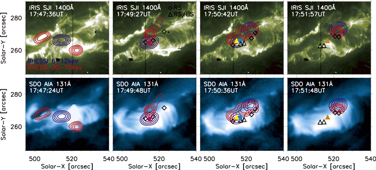
Figure 4. SJI images in the Si iv 1400 Å filter (top, showing the flare ribbons) and AIA 131 Å images (bottom, showing the flare loops) of the 2014 March 29 flare for different times during the evolution of the flare, from left to right. The blue and red contours show the 60%, 70%, 80%, and 90% of the maximum intensity of RHESSI images formed in the 6–12 keV and 30–70 keV energy intervals, respectively, as indicated by the legend. The symbols show the locations where we observe mainly redshifts (diamonds) or both blue and redshifts (triangles) in the Fe xxi spectra. The colored symbols indicate the pixels where we observe the spectra which are plotted in Figures 5 and 6.
Download figure:
Standard image High-resolution imageThe colored contours represent the 60%, 70%, 80%, and 90% of the maximum intensity of the RHESSI images in the 6–12 keV (blue) and 30–70 keV (red) energy intervals. The RHESSI images in Figure 4 were taken during the time intervals (from left to right): 17:46:45–17:47:45 UT, 17:48:45–17:49:45 UT, 17:50:20–17:51:20 UT, and 17:52:10–17:53:10 UT, respectively, using the CLEAN algorithm, as mentioned in Section 2.4. The 6–12 keV images are dominated by thermal emission from the flare loops while the 30–70 keV contours show the location of the HXR sources. The symbols overlaid on the second, third, and forth rows of Figure 4 indicate the pixels where we observe redshifts (diamond symbols) and simultaneous blue and redshifts (triangle symbol) in the Fe xxi spectra. The analysis of the Fe xxi spectra at some of these locations (indicated by a colored diamond or triangle symbol) are shown in Figures 5 and 6.

Figure 5. Left: IRIS Fe xxi CCD detector images at the locations indicated by the symbols in Figure 4. The CCD images are in a negative color scale. The horizontal yellow dotted lines indicate the pixels over which we average the Fe xxi spectrum. Right: Fe xxi spectra showing the redshifts indicated by the red arrows in the corresponding left panels.
Download figure:
Standard image High-resolution imageThe first column of Figure 4 shows the flare at a couple of minutes before the first observation of the redshifts at the top of the loop arcade (≈17:47 UT). The two 30–70 keV RHESSI HXR sources are co-spatial with the location of the flare ribbons, in agreement with the standard scenario of thick-target Bremsstrahlung emission from the flare footpoints (see e.g., Battaglia et al. 2015, who analyzed the same flare event), whereas the 6–12 keV thermal emission appears to originate from the flare loops.
By around 17:49:30 UT (second column), the HXR footpoint sources are not observed anymore in the RHESSI images, whereas a 30–70 keV source appears at the top of the loop arcade, co-spatially with the locations of the Fe xxi redshifts (diamond symbols). We analyzed carefully the X-ray source motion in several energy bands to make sure that this emission is not an effect due to pileup. The fact that the nonthermal and thermal emission are co-spatial usually suggests that the emission originates from the corona. As mentioned in Section 2.4, the spectral analysis showed that the X-ray emission above 25 keV is mostly nonthermal. The 30–70 keV RHESSI coronal source thus likely indicates the presence of nonthermal electrons, which we speculate might have been accelerated by the TS above the loop (see the cartoon in Figure 1). It should be noted that no significant HXR emission is observed at this time at the footpoints. One possible explanation is that the electrons may be "trapped" in the corona without being able to reach the chromospheric footpoints, creating a so-called "coronal thick-target" source (e.g., Krucker et al. 2008 and references therein). We estimated the density required to create a thick target in the corona to be around 1011 cm−3. For this estimate, we used an average electron energy of 30 keV and assumed that the distance traveled by the electrons along the half loop leg (from the loop apex to the footpoints, assuming circular loops) is around 20'', given the distance between the ribbons in the SJI images in Figure 4. The estimated density of the X-ray looptop source for our X1.0-class flare is consistent with the values measured by Simões & Kontar (2013) ((0.6–2.7) × 1011 cm−3) for four X and M class flares and (considering that the density may be smaller for less energetic flares) Chen et al. (2015) ((2–4) × 1010 cm−3) for a C-class flare. Several explanations have been suggested by these authors to explain the excess of nonthermal electrons in the corona. In particular, Simões & Kontar (2013) discussed the possibility of magnetic trapping and/or pitch-angle scattering, which would cause the electrons to be trapped inside the coronal loops without reaching the chromosphere. Turbulent magnetic field fluctuations can also cause electron trapping (Kontar et al. 2014; Musset et al. 2018). In addition, Chen et al. (2015) showed the presence of many small-scale density fluctuations in the TS that may cause the electrons to be repeatedly accelerated each time they pass through the shock. Although it is not possible to distinguish observationally between the different possible scenarios described above, they all provide a plausible explanation for the observation of a nonthermal source in the corona without the corresponding footpoint sources, and are compatible, or do not disagree, with the presence of a TS above the loops.
The third column of Figure 4 shows the flare at ≈17:50:30UT, about 1 minute after the redshifts were first observed. The 30–70 keV coronal source is still present and has now a more similar shape to the 6–12 keV emission from the flare loops, but with a slightly different orientation. At around this time, simultaneous blue and redshifts are observed in the Fe xxi spectra at the flare looptops in different locations, which are indicated by the triangle symbols. Finally, the fourth column shows the flare at around 17:52 UT, when some faint red and simultaneous red and blueshifts are still observed. The location of maximum intensity of both RHESSI images now seems to have shifted eastward along the flare arcade, possibly indicating that reconnection is taken place at a different location than previously observed. Some of the Fe xxi shifts are co-spatial with the new location of the X-ray sources, whereas some faint shifts are still observed in the south-west part of the arcade, where the RHESSI sources are not clearly visible anymore. One possible explanation is that the accelerated electrons are still present there, but that their emission is too faint to be observed by RHESSI.
In Figures 5 and 6, we show in more details some of the Fe xxi spectra, whose position is indicated by the colored filled symbols in Figure 4. For each row of Figure 5, the left panels show the Fe xxi CCD image (left, in negative color scale) and the overlaid red arrow indicates the location of the faint redshift in the Fe xxi line. We note that the Fe xxi spectrum is dominated by the bright and broad at-rest emission from the flare looptops, whereas the redshifted emission can only be observed as a red wing on the Fe xxi line profile. We averaged the Fe xxi spectra over the pixels where the red wing is more intense, between the two horizontal dotted yellow lines overplotted on the detector images, and the resulting spectra are shown on the corresponding right panels. The top panels present the Fe xxi results for one of the first observations of redshifts at the looptop arcade, at the pixels indicated by the pink diamond sign in the second column of Figure 4, whereas the bottom panels of Figure 5 indicate a redshift which is observed later on, during raster 177 and exposure 2, at the location indicated by the light-blue diamond in the third column of Figure 4. Both observations show Fe xxi redshifts of about 200 km s−1, but in the second case (bottom panel of Figure 5), the redshifted profile is more intense and its profile is clearly separated from the main at-rest Fe xxi component.

Figure 6. Left: IRIS Fe xxi CCD detector images at the locations indicated by the symbols in Figure 4. The CCD images are in a negative color scale. The horizontal yellow dotted lines indicate the pixels over which we average the Fe xxi spectrum. Right: Fe xxi spectra showing the blue and redshifts indicated by the red and blue arrows in the corresponding left panels. The insert in the top left panel shows a zoom into the blue side of the Fe xxi spectrum, where we identified the broad Fe xxi blueshited emission and the narrow photospheric line blends.
Download figure:
Standard image High-resolution imageFigure 6 shows the Fe xxi spectra in two of the locations where we observe simultaneous faint red and blue wings in the line profile, indicated by the yellow and orange triangles in Figure 4. Similar to Figure 5, the red (blue) arrow indicates the red (blue) wing. The spectra in Figure 6 show that the red wing component has a velocity of about 200 km s−1, similar to the spectra in Figure 5, whereas the blue wing has a Doppler velocity of about −250 km s−1. The insert in the top panel of Figure 6 shows a zoom in the blue side of the Fe xxi spectra, which we fitted by including the identified photospheric lines in that part of the spectrum, as observed by Sandlin et al. (1986). The fit shows that even taking into account these narrow lines, a broad (i.e., high temperature) emission line is still needed to properly fit the blue side of the Fe xxi spectrum, which we interpret as a blueshifted Fe xxi component. Note in fact that, apart from the Fe xxi line, only cool (photospheric and chromospheric) lines are observed in this spectral interval, as observed by e.g., Sandlin et al. (1986), Brekke et al. (1991). In particular, we note that the unidentified line at around 1352.5 Å in our spectrum is most likely the H2 transition identified by Jaeggli et al. (2018).
Blueshifts in Fe xxi lines can also be caused by chromospheric evaporation in flares (e.g Graham & Cauzzi 2015; Polito et al. 2015, 2016; Tian et al. 2015; Young et al. 2015; Tian & Chen 2018). However, our blueshifts lack some of the typical characteristics observed in the chromospheric evaporation flows, such as a persistent blueshift of the line which can last several minutes (e.g., Graham & Cauzzi 2015; Polito et al. 2015, 2016; Reep et al. 2018), the typical pattern of decreasing blueshifts away from the ribbons (e.g., Young et al. 2015; Tian & Chen 2018) and the fact that the blueshifts are usually accompanied by strong (i.e., ≈40–100 km s−1) redshifts in the Si iv line in the same location (e.g., Tian & Chen 2018). Further evidence that the observed blueshifts are not caused by evaporating upflows may be found by analyzing the spectra of other lines included in the IRIS spectra, as discussed in Section 4.
4. Other IRIS Lines
We also analyzed cooler lines observed by IRIS, in particular the transition region Si iv 1402.77 Å and photospheric/chromospheric Fe i 2814.11 Å and Fe ii 2814.45 Å lines. From left to right, Figure 7 shows the CCD images of Si iv, Fe ii and the closet in time SJI 1400 Å and SDO/HMI line-of-sight magnetic field images of the flare. The top panel of Figure 7 shows CCD images (and simultaneous SJI and HMI images) during the raster 177, exp 2, which can be directly compared with the bottom panel of Figure 5, where we observe redshifts in the Fe xxi spectra. Similarly, the bottom panel of Figure 7 can be directly compared with the Fe xxi spectra in raster 178, exp 2, at the location where we observe both blue and redshifts, as shown in the bottom panel of Figure 6. Figure 7 shows that the same place where we observe the Fe xxi redshifts and simultaneous blue/redshifts, the Si iv line is very intense, and modestly redshifted of about 15 km s−1. In addition, in raster 178, exp 2, the line profile shows a central reversal, which is typically observed when the line is formed under optically think emission. The corresponding SJI images (and AIA images in cool filters, such as 304 Å, not shown here) suggest that the this emission originates from loop structures rather than ribbons. This is also confirmed by the fact that the photospheric emission in Fe i and Fe ii (likely originating from the southern ribbon) is well separated along the slit from the redshifted intense Si iv emission, and by the lack of strong magnetic features observed in simultaneous HMI line-of-sight images, which typically mark the location of the ribbons. Therefore, we interpret the redshifted and intense Si iv emission as coming from cool loops (also observed in cool AIA bands), which are likely caused by the gradual cooling of plasma previously heated to million degrees during the impulsive phase of the flare. This suggests that we are observing superposition of both flare loops which are still being energized (and emit in Fe xxi–Fe xxiii temperatures) and cooling plasma (emitting over a large range of temperatures) from previously heated loops.

Figure 7. From left to right: CCD images of the Si iv 1402.77 Å and Fe ii 2814.45 Å spectral windows during the exposure no. 2 of the IRIS rasters 177 (top panels) and 178 (bottom panels) and closest AIA and HMI images in time. The yellow horizontal lines in the top and bottom panels are the same as the ones shown in the corresponding images in Figures 5 and 6, and indicate the location where we observe redshift only or simultaneous redshift and blueshift in the Fe xxi, respectively. The pink line marks the IRIS slit position.
Download figure:
Standard image High-resolution imageIn addition, we note that during large flares photospheric and chromospheric lines at the ribbons can become significantly brighter, broaden, and sometimes show significant redshifts (Kowalski et al. 2017). To rule out significant contamination from cool lines to the Fe xxi redshifted and blueshifted profiles, we take a closer look at the spectra of the Fe i and Fe ii lines in Figure 7. In particular, the Fe ii line is formed at the same temperature as the Fe ii lines around 1354 Å on the red side of the Fe xxi spectra, which could potentially contaminate the redshifted Fe xxi emission. As mentioned before, Figure 7 shows that the region where the cool Fe i and Fe ii lines are most intense seems to coincide with the location of the continuum emission from the ribbon in Figures 6 and 5, and is well separated from the position where we observe the Fe xxi looptop shifts (which is indicated by the yellow horizontal lines in the figure). We conclude that the strongest photospheric and chromospheric emission comes from the ribbons, and therefore does not significantly contaminate the observed Fe xxi spectra at the top of the loop arcade. This conclusion is bolstered by the fits shown in Figure 6, where the Fe ii is only provides a very small contribution to the fit intensity.
5. Discussion and Summary
We have found large redshifts, sometimes occurring simultaneously with fainter blueshifts (with absolute velocities in the range 200–250 km s−1) in the IRIS Fe xxi spectra along several locations at the top of the loop arcade during the X1-class flare on 2014 March 29. The location of the Fe xxi shift are mostly co-spatial with 30–70 keV RHESSI sources, indicating the presence of nonthermal electrons in the corona.
We speculate that the shifted Fe xxi components are the deflection flows predicted by the existence of a TS above the closed loops in flare reconnection models (see Figure 1). The Fe xxi spectra are dominated by the at-rest component from the flare loops and the shifted components appear much fainter (by a factor of ≈30–50) and broader (up to a factor of two) for the X-class flare under study. This might explain the relative paucity of observations of hot plasma flows in the reconnection region, in particular for smaller flares, where the Fe xxi is usually less intense. This argument can be further supported by the fact that the faint shifts are observed over only few IRIS pixels along the slit (5–10 pixels, corresponding to ≈1''–2''), which cannot be easily distinguished by spectrometers such as Hinode/EIS, which have a lower spatial resolution (around 3''–4'', see the Appendix).
Theoretical estimates of typical speeds downstream of TS shocks were recently provided by Guo et al. (2017), who predicted intense Fe xxi redshifted components by around 250–300 km s−1. The deflecting flows should in principle have smaller velocities then the downstream flows, depending on the observing angle along the line of sight. In addition, Yokoyama et al. (2001) predicted velocities for the deflecting flows of around 115 km s−1 (bottom right panel of Figure 3 in their paper). These predicted values seem to be in reasonable agreement with the Doppler velocities (200–250 km s−1) that we found in our observation.
Our results are also consistent with previous observations by Imada et al. (2013), who found blue and redshifts of around 400 km s−1 in the hotter EIS Fe xxiv lines during an X-class flare at the limb, which they interpreted as the parallel flows caused by the TS.
Some aspects of our interpretation require further discussion, and we address them individually in the following:
- 1.Are we observing the flows in the downstream or upstream of the fast-mode shock? We believe that the Fe xxi Doppler shifts are most likely the flows downstream of the shock rather than the reconnection outflows. As already mentioned in the introduction, the plasma in the downstream region is in fact expected to be denser (by around a factor of two; Forbes 1986), and therefore easier to observe, compared to that in the upstream region, which is also more likely outside ionization equilibrium (Imada et al. 2011). Further, our spectra show similar values of blue and redshifts, which is consistent with the observation of deflecting flows due to the fast-mode shocks. In contrast, the speed of the upward and downward reconnection jets may be very different depending on the plasma beta (e.g., Forbes 1986; Reeves et al. 2010). In particular, there is some evidence that the plasma in the supra-arcade region has a beta close to 1 (McKenzie 2013), in which case the downward jet should almost be suppressed (Forbes & Malherbe 1991).
- 2.Why not all the redshifts are accompanied by a corresponding blueshift? It is interesting to note that we do not find simultaneous blueshifts and redshifts at all the locations, but Fe xxi spectra showing only redshifts are sometimes observed. A possible explanation might be related to the fact that the flare under study is oblique, i.e., located between the disk and the limb in the northwest solar hemisphere. For a perfectly on-disk flare, the predicted spectra would only show the downflows which are produced immediately downstream of the shock, and also the deflected flows would be mostly visible as moving away from the observer, i.e., as redshifts/downflows (see also Guo et al. 2017). In our observation, the flare arcade is not completely perpendicular to the LOS (see Figure 1), thus the predicted flows which are deflected around the closed reconnected loops could be observed as simultaneous blueshifts and redshifts. It is possible that we found both these two scenarios in our observations, depending on the inclination of the loops. More specifically, in some pixels we might be seeing only the downstream flows (i.e., the short red arrows in Figure 1), whereas in other pixels we see a superposition of the deflection flows, resulting in the observation of both red and blueshifts. Finally, as mentioned before, the possibility of the redshifts being caused by retracting loops along the line of sight cannot be completely ruled out, given the geometry of the flare almost on-disk.
- 3.Can the Fe xxi spectra be contaminated by evaporating flows or emission from photospheric/chromospheric lines? One could ask whether the observed blueshifts in some of the observed spectra might be a signature of the evaporating upflows from the ribbons rather than of the fast-mode shocks. As discussed in Sections 3 and 4, there is some evidence supporting the idea that the observed blueshift emission does not originate from the ribbons, such as the lack of the typical characteristics (i.e., persistent blueshifts which decrease gradually away from the ribbons, accompanied by strong TR condensation) which are usually observed in the spectra of Fe xxi evaporating flows (e.g., Polito et al. 2016; Tian & Chen 2018). Further, as shown in Figures 5–7, the location of the blue and redshifted components (indicated by the yellow horizontal lines) appears in fact to be well separated along the slit (by at around 30 IRIS pixels or 5'') from the ribbon location (where the strong UV continuum emission appears) and where the cool Fe i and Fe ii emission is strongest.In addition, we examine the possibility that the shifted and very broad Fe xxi emission that we observe might be significantly blended with narrow photospheric lines which are usually observed during flares (e.g., Polito et al. 2016). For instance, for the 2014 March 29 flare under study, Kowalski et al. (2017) observed very broaden and redshifted profiles for the Fe ii line around 2814 Å. These lines are formed at the same temperature (log T ≈ 4.15) as the Fe ii 1354.75 Å and 1354.85 Å lines on the red side of the Fe xxi spectral window, and thus may contaminate the profiles of the hotter Fe xxi line. To rule out this possibility, we analyze the spectra of the Fe ii 2814.45 Å line, which is free from blends from other emission lines. In Figure 7, we plot two CCD images showing the spectra of the Fe ii 2814.45 Å line (and also Fe i 2814.11 Å) during the rasters 177 and 178 and exposure 2. The images are taken at the time we observe some of the Fe xxi red/blueshifts which are shown in Figures 5 and 6. Similar to these latter figures, the yellow dotted horizontal lines indicate the locations of the maximum intensity of the Fe xxi shifted component. By comparing Figure 7 with Figures 5 and 6, we can see that the regions of Fe i and Fe ii bright emission is spatially well separated (by around 5'') from the position where we observe the faint Fe xxi shifts, and instead correspond to the ribbon continuum emission observed in Figures 5 and 6. This shows that the Fe xxi shifts we are observing are likely located at the flare loops top and are not contaminated by ribbon emission from neighboring cool lines such as Fe i and Fe ii.
- 4.Why are the flows observed in the peak/gradual phase of the flare? We note that the observed large flows appear during the peak/gradual phase of the flare and not during the impulsive phase. This occurrence is not surprising, as the Fe xxi blueshifts from the flare ribbons (chromospheric evaporation) are observed until at least six minutes after the peak of the flare (Young et al. 2015), suggesting that the heating deposition and/or particle acceleration (and therefore magnetic reconnection) is still going on during the gradual phase. As long as reconnection continues and the outflow jets are created, the fast-mode shocks can occur. Also, the impulsive phase of the flare under study appears to be very rapid, therefore it may take some time for the plasma to reach a high enough density for any significant Fe xxi emission to be visible.
We performed a detailed search for flare events showing large Doppler shifts in the IRIS Fe xxi high-temperature line observed above the looptops, and selected the March 29 X-class flare for further investigation. Finding a clear observation of such shifts is complicated by the fact that the line is hard to observe where the density of the emitting plasma is low, such as in the reconnection region, therefore only a few suitable flare events were found. Thanks to the high spatial resolution of the IRIS spectrograph channel, we were able to separate spatially the emission from the flare loops and ribbons for a non-limb flare. The observations we have presented in this work strongly support the magnetic reconnection scenario in flares and the possible presence of a TS above the flare loops.
Our work highlights the need of future spectroscopic observations of strongly emitting high-temperature lines at very high spatial and temporal resolution, which are crucial to better investigate the dynamics of the reconnection region. The observational advancements must also be accompanied by improvements in the theoretical models of reconnection in flares, which should be able to predict specific observables (i.e., spectra observed by current instruments, see e.g., Guo et al. 2017) for a large variety of physical parameters and geometries, such as oblique flares as the one presented in this work.
We thank the referee for the useful comments which helped improving the manuscript. V.P. is supported by the NASA grants NNX15AJ93G and NNX15AF50G, and by contract 8100002705 from Lockheed-Martin to SAO. G.G. is supported by the NSF-REU Solar Physics program at SAO, grant number AGS-1560313 and NASA grant NNX15AJ93G. K.R. is supported by the NASA grant NNX15AJ93G. The authors thank Dr. Lynsday Gleneser for insightful discussions. IRIS is a NASA small explorer mission developed and operated by LMSAL with mission operations executed at NASA Ames Research center and major contributions to downlink communications funded by ESA and the Norwegian Space Center. AIA data are courtesy of NASA/SDO and the respective science teams. Hinode is a Japanese mission developed and launched by ISAS/JAXA, with NAOJ as domestic partner and NASA and STFC (UK) as international partners. It is operated by these agencies in co-operation with ESA and NSC (Norway).
Appendix: A Note on the Hinode/EIS Observations
On 2014 March 29 Hinode/EIS observed the X1-class flare under study during a 11-step raster targeting the AR NOAA 12017, as described in Section 2.1. The raster study had a very limited selection of spectral lines, and did not include emission lines which provide crucial information during flares, such as Fe xxiv and Fe xiv. The EIS raster was also coarse sparse, with a slit width of 1'' and a jump of 3'' between each exposures. Figure 8 shows intensity images of the Fe xxiii (T ≥ 10 MK) and Fe xvi (T ≥ 3 MK) lines observed by EIS, which were obtained by fitting the lines with a single Gaussian profile at each pixel. The images on the left panel do not include any corrections for the sparse raster, but are obtained by assuming (for convenience) that the slit width was 4''. The right panel instead shows what portion of the flare arcade EIS is actually observing. The vertical dotted lines indicate the IRIS slit positions 0–5, where we observe the Fe xxi shifts, and the pink line highlights a location that both spectrometers were observing (within the alignment uncertainty) and that we select as an example for further investigation. Figure 9 compares the IRIS Fe xxi and EIS Fe xxiii and Fe xvi CCD images (from left to right, respectively) at this location. The colored arrows in Figure 9 indicate the location of the ribbon (light-blue arrow) and the redshifted component in the Fe xxi spectrum (red arrow). Figure 10 shows the line profiles of Fe xxiii 263.78 Å, Fe xvi 262.98 Å and Fe xvii 269.42 Å at those two locations (as indicated by the light blue or red colors of the spectra, respectively). The vertical line in each panel indicate the at-rest position of the lines, obtained by measuring the centroid position of the Fe xvi line outside of the flaring area. These reference position are however estimated with a large uncertainty: because of the lack of absolute reference wavelengths (as provided by neutral lines) in the EIS spectra, as well as some well-known issues (such as the spectral tilt along the slit6 ), this uncertainty can be as high as ≈15 km s−1. The spectra in Figure 10 show that the dominant component of the lines is at rest or almost at rest, considering the uncertainty in the wavelength calibration. The ribbon emission observed in the IRIS spectra mostly coincides with an increased blue wing emission in the EIS Fe xxiii line, which we interpret as the evaporating flows from the flare footpoints. A possible faint blue wing emission may also be observed in the light-blue Fe xvi spetrum in Figure 10, but not in the Fe xvii line, indicating that it might not be real, given the very low spectral points along the blue side of the Fe xvi line profile. In contrast, no significant redshifted emission is observed in Fe xxiii (or in the Fe xvi and Fe xvii spectra). There are different possible explanations for this. First, EIS is observing a very limited portion of the flare loop arcade, and the two spectrometers are probably not observing the same location, due to the 3'' jump of the EIS observations and the co-alignment uncertainties. In addition, the timing of the two observations differs by about one minute, and we do not observe the redshifts in the Fe xxi spectra to persist for more than 75 s (the cadence of the IRIS raster) in the same location. The fact that the Fe xxi shifts appear to be observed at different locations over time above the looptops suggest that they might have been missed by the EIS spectrometer which has a slower raster cadence (about 130 s) and a large 3'' jump between exposures. Further, the redshifted emission that we identify at the looptop and the ribbon emission are separated by about 4''–5'', which corresponds to only 1–2 pixels in EIS (which has a point-spread function of about 3''–4''), and therefore might be harder to separate spatially by this latter instrument. Further, it is possible that the redshifted component for the EIS Fe xxiii line might have a larger velocity than those of the Fe xxi line observed by IRIS (for instance, as mentioned before Imada et al. 2013 found shifts up to 400 km s−1 in the EIS Fe xxiv lines) and thus could lie outside the EIS spectral window. Finally, we note that the spectral lines in Figure 10 show non-Maxwellian profiles with pronounced wings. Similar profiles were also found at both ribbons and flare loops at different times by Jeffrey et al. (2017), who analyzed the 2014 March 29 flare under study and by Polito et al. (2018) during another X-class flare. These authors interpreted the non-Gaussian line profiles as signatures of ions acceleration and plasma turbulence, which are also compatible with the presence of a TS.

Figure 8. Intensity maps of the EIS Fe xxiii line (reversed color scale) showing the emission from the hot loop arcade without and with the sparse raster correction applied (left and right panels, respectively). The horizontal dotted lines show the IRIS slit positions 0–5 for the 8-step IRIS raster. The pink horizontal line highlights the location corresponding to the IRIS and EIS CCD images shown in Figure 9. The images are saturated to bring up the less fainter spectral features.
Download figure:
Standard image High-resolution image
Figure 9. IRIS (left panel) and EIS (middle and right panel) CCD images showing the Fe xxi 1354.08 Å, Fe xxiii 263.78 Å and Fe xvi lines at the location indicated by the pink dotted line in Figure 8. The horizontal arrows in both panels show the position of the ribbon emission (light blue) and the redshifts (red) observed in the IRIS Fe xxi spectra.
Download figure:
Standard image High-resolution image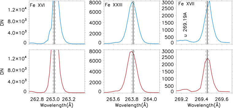
Figure 10. Fe xiv (left), Fe xxiii (middle) and Fe xvii (right) spectra at the locations indicated by the light-blue and red arrows in Figures 8 and 9, respectively. The vertical black line shows the position of at-rest position of the lines respectively (obtained using the Fe xvi intensity outside the flaring region as absolute wavelength reference), with associated ±15 km s−1 uncertainty (dotted gray lines).
Download figure:
Standard image High-resolution image
The comparison with the EIS spectra confirms what already mentioned in Section 5, that the presence of faint redshifted components in high-temperature lines might be difficult to identify in the case of non-limb flares for observations with limited spatial resolution and coverage and low temporal cadence, as in the case of the EIS study analyzed here. We conclude that for this particular study the EIS observations do not provide conclusive information either confirming or ruling out our interpretation of blue and redshifts of Fe xxi as possible signatures of TS deflecting flows. This is partially due to the limited spatial resolution of the spectrometer, but also to the low cadence and limited spatial coverage of the coarse sparse raster of this study, as well as the limited wavelength range of the spectral window on the red side of the Fe xxiii line.
Footnotes
- 4
- 5
- 6