


Abstract
Up to now several gravitational-wave events from the coalescences of black hole binaries have been reported by LIGO/VIRGO, and imply that black holes should have an extended mass function. We work out the merger rate distribution of primordial black hole (PBH) binaries with a general mass function by taking into account the torques by all PBHs and linear density perturbations. In the future, many more coalescences of black hole binaries are expected to be detected, and the one-dimensional and two-dimensional merger rate distributions will be crucial for reconstructing the mass function of PBHs.
Export citation and abstract BibTeX RIS
It is believed that primordial black holes (PBHs) could have formed in the early Universe from the collapse of large density fluctuations (Hawking 1971; Carr & Hawking 1974; Carr 1975). On the other hand, one of the challenges for fundamental physics is the understanding of the nature of dark matter (DM). Among a large variety of models, the speculation that the DM is composed totally or partially by PBHs has attracted much attention, especially since the discovery of black hole coalescence by LIGO (Abbott et al. 2016a), because the coalescence of PBH binaries can be candidates for the observed gravitational-wave events (Bird et al. 2016; Sasaki et al. 2016).
Up to now, there are several gravitational-wave events from binary black hole (BBH) mergers reported by LIGO and VIRGO collaborations: GW150914 ( ,
,  ) (Abbott et al. 2016a), GW151226 (
 ,
,  ) (Abbott et al. 2016d), GW170104 (
 ,
,  ) (Abbott et al. 2017d), GW170608 (
 ,
,  ) (Abbott et al. 2017a), GW170814 (
 ,
,  ) (Abbott et al. 2017c), as well as a less significant candidate, LVT151012 (
 ,
,  ) (Abbott et al. 2016e, 2016f). These events indicate that the black holes should have an extended mass function. In fact, the generic initial conditions of PBH formation also suggest that the PBH mass should also extend over a wide range.
In the literature there are two main paths for the PBH binary formation. One is formed in the early Universe (Nakamura et al. 1997; Sasaki et al. 2016; Ali-Hamoud et al. 2017) and another is formed in the late Universe (Bird et al. 2016; Ali-Hamoud et al. 2017; Nishikawa et al. 2017), respectively, and the former generically makes the dominant contribution to the PBH merger rate. However, the mass function of PBHs is usually assumed to be monochromatic in Sasaki et al. (2016), Nakamura et al. (1997), Ali-Hamoud et al. (2017), Bird et al. (2016), and Nishikawa et al. (2017). Recently, the merger rate of PBHs with an extended mass function is investigated in Raidal et al. (2017) and Kocsis et al. (2018), but only the tidal force from the PBH closest to the center of mass of the PBH binary is taken into account in Raidal et al. (2017) and a flat mass function of PBHs over a small mass range is considered in Kocsis et al. (2018).
In this paper we consider the torques of all PBHs and linear density perturbations, and calculate the merger rate distribution for the PBH binaries with a general mass function. In the upcoming decades, many more BBH mergers are expected to be detected, and they will provide better information about the black hole mass function; this may finally help us answer the question: What is the origin of black holes, and how are black hole binaries formed in our Universe?
The probability distribution function (PDF) of PBHs, P(m), is normalized to be

and the abundance of PBHs in the mass interval,  , is given by

where f is the total abundance of PBHs in nonrelativistic matter. In this paper, for convenience, the PBH mass is in units of  . The fraction of PBHs in cold DM is related to f by
  . We introduce a cross-grained discrete PDF, namely

where  is the binned PDF and
  denotes the resolution of the PBH mass. Roughly speaking,
  is taken as the abundance of PBHs with mass mi. At matter-radiation equality the total energy density of matter is

and then the average distance,  , between two PBHs with mass mi is

which depends on both mass mi and its abundance  . We need to stress that the number densities for PBHs with different masses can be quite different from each other, and in principle, there is no well-defined number density for the overall PBHs. The average distance,
  , between two neighboring PBHs with different masses mi and mj is estimated as

where

and


The above formula are valid for  , and can be generalized to cover
  if we take
  . From now on, for simplicity, we omit the subscript ij unless it is necessary.
In order for the formation of a PBH binary, the two neighboring PBHs necessarily decouple from the background expansion and form a bound system. In Newtonian approximation, the equation governing the evolution of the proper separation, r, of the black hole binary with masses mi and mj along the axis of motion takes the form

where the dot denotes the derivative with respect to the proper time. In this paper we work in the geometric units  . Defining
  , we rewrite Equation (11) as
where x is the comoving separation between these two PBHs, primes denote the derivative with respect to scale factor s, which is normalized to be unity at equality, and  . Here the dimensionless parameter
  is
is
where

and  is given in Equation (8). The solution of Equation (12) in Ali-Hamoud et al. (2017) implies that the decoupling occurs before the equality if
  and the semimajor axis a of the formed binary is given by

Without the tidal force from other PBHs and density perturbations, these two PBHs will just collide head-on with each other. However, the tidal force will provide an angular momentum to prevent this system from direct coalescence. For simplicity, we introduce a dimensionless angular momentum, j, defined by

where ℓ is the angular momentum per unit reduced mass and ![$e\in [0,1]$](https://content.cld.iop.org/journals/0004-637X/864/1/61/revision1/apjaad6e2ieqn31.gif) is the eccentricity. In order to estimate the initial orbital parameters for the PBH binary in which two PBHs can have different masses, we generalize the method in Ali-Hamoud et al. (2017). Here we do not plan to repeat all of the calculations in Ali-Hamoud et al. (2017), but only highlight the key results. The local tidal field is related to the Newtonian potential ϕ by
is the eccentricity. In order to estimate the initial orbital parameters for the PBH binary in which two PBHs can have different masses, we generalize the method in Ali-Hamoud et al. (2017). Here we do not plan to repeat all of the calculations in Ali-Hamoud et al. (2017), but only highlight the key results. The local tidal field is related to the Newtonian potential ϕ by  which exerts a perturbative force per unit mass
  . Supposing that the initial comoving separation of the binary is small relative to the the mean separation, this tidal force does not significantly affect the orbit of the binary, but it produces a torque which yields

Since the tidal field generated by other PBHs and density perturbation in the radiation-domination era is  ,
,  and then
where  is the unit vector along
  and
and  is the local tidal field at equality. The tidal field generated by a PBH with mass ml at a comoving separation
  is given by
and then
Similar to Ali-Hamoud et al. (2017), following Chandrasekhar (1943), the two-dimensional PDF of j from torques by all other PBHs is given by
where  is total number of PBHs with mass ml,

and  and
and  . After a tedious computation, we find

Since  is the energy density of PBHs with mass ml,
  and then

where
which encodes the torques by all other PBHs. Integrating over Equation (24) gives
where  . In addition, the variance of
  due to the torques by density perturbations is
where  is the variance of density perturbations of the rest of DM on a scale of the order of
  at equality. Taking into account both the torques by all of other PBHs and density perturbations, the characteristic value of jX in Equation (26) reads as
After the formation of a PBH binary, the orbit of these two binary PBHs shrinks due to the gravitational waves, and the coalescence time is given by Peters (1964) as
Taking into account Equation (15), the dimensionless angular momentum is
Assuming that PBHs possess a random distribution, the probability distribution of the separation, x, between two nearest PBHs with mass mi and mj and without other PBHs in the volume of  becomes

where  , μ is given in Equation (7), and
  .5
Therefore we have
.5
Therefore we have
where jX is given in Equation (28). The probability distribution of the time of merger becomes

and the comoving merger rate at time t reads as
where  is the matter density at present. Since
  has a sharp peak at
if  ,6
the comoving merger rate at time t becomes
,6
the comoving merger rate at time t becomes

where
which can be interpreted as the comoving merger rate density in units of Gpc−3 yr−1, and PBH masses are in units of  . Again, we want to remind readers that
  for
for  . If
. If  constant,
  , which is consistent with Kocsis et al. (2018). However, for a general mass function,
  can be quite different from 36/37.
Let's consider two typical PBH mass functions in the literature. One takes the power-law form (Carr 1975)

for  and
and  , and the other has a lognormal distribution (Dolgov & Silk 1993) of
LIGO/VIRGO gives the merger rate for BBHs with  and
and  as
as  Gpc−3 yr−1 in Abbott et al. (2017d). Similar to Ali-Hamoud et al. (2017), we take
  . Figure 1 indicates that the merger rate constrained by LIGO/VIRGO can be explained by mergers of PBH binaries. Here, for the purpose of illustration, we simply take
  and
and  for the power-law PDF, and
  and
and  for the lognormal PDF. Therefore LIGO/VIRGO implies that
  for the power-law PDF and
  for the lognormal PDF. Such an abundance of PBHs is consistent with current constraints from other observations (Chen et al. 2016; Green 2016; Horowitz 2016; Ali-Hamoud & Kamionkowski 2017; Aloni et al. 2017; Carr et al. 2017; Clesse & García-Bellido 2017; Gaggero et al. 2017; Green 2017; Guo et al. 2017; Inoue & Kusenko 2017; Khnel & Freese 2017; Schutz & Liu 2017; Zumalacarregui & Seljak 2017; Wang et al. 2018). In order to break the degeneracy for different PBH mass functions, we need more information. Keeping the total merger rate of RT = 100 Gpc−3 yr−1 fixed, we obtain
  for the power-law PDF and
  for the lognormal PDF, respectively, and then plot the one-dimensional merger rate distribution (where we integrate the mass of the lighter black hole in the binary from
  over the mass of the heavier black hole) in Figure 2. We see that one-dimensional merger rate distributions for the lognormal and power-law PDFs are quite different from each other even though both PDFs give the same total merger rate, RT. Furthermore, more information will be obtained in the two-dimensional merger rate distributions in Figure 3.
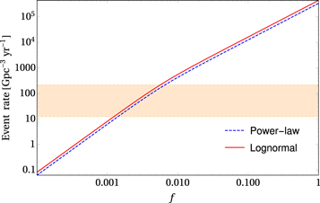
Figure 1. Merger rate of PBH binaries at present with  and
and  . The blue dotted and red solid lines correspond to the power-law PDF (
 and
and  ) and lognormal PDF (
 and
and  ), respectively.
Download figure:
Standard image High-resolution image
Figure 2. One-dimensional merger rate distribution, where mH is the mass of the heavier black hole in the binary and the mass of the lighter black hole is integrated over from  to mH. The blue dotted and red solid lines correspond to the power-law PDF (
 and
and  ) with
  and lognormal PDF (
 and
and  ) with
  , respectively.
Download figure:
Standard image High-resolution image
Figure 3. Two-dimensional merger rate distributions. The top and bottom panels correspond to the power-law PDF ( and
and  ) with
  and lognormal PDF (
 and
and  ) with
  , respectively.
Download figure:
Standard image High-resolution imageIn order to compare to the events detected by LIGO, we need to take the sensitivity of LIGO into account. Since LIGO probes mergers approximately in the redshift range of ![$z\in [0,1]$](https://content.cld.iop.org/journals/0004-637X/864/1/61/revision1/apjaad6e2ieqn100.gif) , the expected number of triggers, Λ, is therefore estimated as (Abbott et al. 2016c, 2016b, 2017b; Kavanagh et al. 2018)
, the expected number of triggers, Λ, is therefore estimated as (Abbott et al. 2016c, 2016b, 2017b; Kavanagh et al. 2018)

where  is the averaged sensitive spacetime volume of LIGO, which depends on the masses of the merging BBH. We adopt the semi-analytical approximation presented in Veitch et al. (2015), Abbott et al. (2016b, 2016c), and Usman et al. (2016) to calculate
  . Here we assume LIGO's O1 and O2 runs share a common sensitive volume, with an observing time of 48.6 days for O1 (Abbott et al. 2016e) and 117 days for O2 (Abbott et al. 2017e). Note that Λ is not the mean number of confidently detected BBH events, but the mean number of signals above the chosen threshold (Abbott et al. 2016c). The two-dimensional distributions of Λ, along with the six events detected by LIGO/VIRGO, are then shown in Figure 4. Since there are only a few events available so far, we cannot make a decisive conclusion as to which PDF fits the data better. As the data accumulating, we may finally pin down the shape of the black hole mass function and nail down whether lower and/or upper mass cutoffs (Fishbach & Holz 2017; Kovetz et al. 2017) of merging black hole binaries exist or not.

Figure 4. Two-dimensional distributions for Λ (see Equation (40)), along with the six events detected by LIGO/VIRGO. The crosses indicate error bars for each event. The top and bottom panels correspond to the power-law PDF ( and
and  ) with
  and lognormal PDF (
 and
and  ) with
  , respectively.
Download figure:
Standard image High-resolution imageIn this paper we work out the merger rate distribution of PBH binaries with a general mass function, taking into account the torques by all other PBHs and the linear density perturbations. In Ali-Hamoud et al. (2017), the effects of the tidal field from the smooth halo, the PBH binary encountering with other PBHs, the baryon accretion, and present-day halos were carefully investigated, and they concluded that all of these effects make no significant contribution to the overall merger rate. So it is reasonable for us to neglect these subdominant effects throughout our estimation as well. In addition, we find that the evolution of the merger rate of PBH binaries is  , which is quite different from that for the astrophysical black hole binaries.
For the power-law and lognormal cases, the abundance of PBH is roughly constrained to the range of  , which is consistent with other observations (Chen et al. 2016; Green 2016; Horowitz 2016; Ali-Hamoud & Kamionkowski 2017; Aloni et al. 2017; Carr et al. 2017; Clesse & García-Bellido 2017; Gaggero et al. 2017; Green 2017; Guo et al. 2017; Inoue & Kusenko 2017; Khnel & Freese 2017; Schutz & Liu 2017; Zumalacarregui & Seljak 2017; Wang et al. 2018). Our results hence confirm that the dominant fraction of DM should not originate from the stellar mass PBHs (Sasaki et al. 2016; Ali-Hamoud et al. 2017; Raidal et al. 2017; Kocsis et al. 2018).
A possible method to discriminate a PBH scenario from the others is to measure the merger rate distribution of black hole binaries. In particular, we show that the one-dimensional and two-dimensional merger rate distributions are quite sensitive to the mass function of PBHs. In the near future, many more coalescences of black hole binaries will be detected and provide the distribution of the binary parameters, and hence the mass function of a PBH (or black hole) could be reconstructed from the one-dimensional and two-dimensional merger rate distributions. This may finally help us answer the questions: What is the origin of black holes detected by LIGO and VIRGO collaborations and how are black hole binaries formed?
We thank the anonymous referee for valuable suggestions and comments. We acknowledge the use of the HPC Cluster of ITP-CAS. This work is supported by grants from NSFC (grant No. 11335012, 11575271, 11690021, 11747601), Top-Notch Young Talents Program of China, and partly supported by the Strategic Priority Research Program of CAS and Key Research Program of Frontier Sciences of CAS.

