


Abstract
Observations from the Ion and Neutral Camera (INCA) on the Cassini mission of energetic neutral atoms (ENAs) at ∼10 keV and ∼45 keV showed significant correlated time variations over relatively fast 2–3 yr timescales. These observed ENA variations have been interpreted as indicating limited scale lengths of ∼80–120 au along the line of sight for the size of the heliosphere. We show here, however, that rather than a heliosphere with a quasi-spherical shape, the INCA line-of-sight observations vary in response to episodic cooling and heating of the inner heliosheath plasma during periods of large-scale expansion and compression.
Export citation and abstract BibTeX RIS
1. Introduction
There is ongoing active research on the shape of the heliosphere, the region of space carved from the local interstellar medium (LISM) by the solar wind's strong radial expansion. Parker (1961) described two paradigms for the shape in the heliosphere and other astrospheres. In the first paradigm, in response to the interstellar nonmagnetized flow, the heliosphere takes a comet-like shape with a long tail, much like a wind sock. A long history of analytic modeling (Baranov et al. 1970; Wallis 1973; Baranov et al. 1976; Baranov 1990, 2000) and numerical modeling (Baranov et al. 1981; Osterbart & Fahr 1992; Baranov & Malama 1993; Baranov & Zaitsev 1995; Zank et al. 1996, 2001; Pogorelov & Semenov 1997; Linde et al. 1998; Pogorelov & Matsuda 1998; Ratkiewicz et al. 1998, 2002; Washimi & Tanaka 1999; Alexashov et al. 2000; Fahr et al. 2000; Pogorelov et al. 2004, 2006, 2009, 2015; Heerikhuisen et al. 2006, 2008, 2014; Malama et al. 2006; Izmodenov et al. 2009; Izmodenov & Alexashov 2015) has shown strong support for this comet-like model of the heliosphere.
Parker (1961) considered also a second paradigm for the heliosphere (hereafter Parker type II). He suggested that in the limit of a strong interstellar magnetic field and a stationary Sun, the shape of the heliosphere is quite different from comet-like. Instead of a single well-defined tail, the heliosphere has outflow along the two poles of the interstellar magnetic field.
The wake (or tail) of the heliosphere was studied by Yu (1974). In this case, the solar wind's spiral magnetic structure defines two lobes of the heliosphere's tail. Recent magnetohydrodynamic (MHD) modeling (Opher et al. 2015) and an analytic model (Drake et al. 2015) have also shown results consistent with multiple jet-like lobes. A two-lobe structure of the heliosphere was also obtained by Czechowski & Grygorczuk (2017) from MHD modeling for the case of a strong interstellar magnetic field (B > 10 μG) in which the Sun moves with respect to the strongly magnetized interstellar matter—a generalization of the original analytic solution by Parker (1961).
The Parker type II solution is obtained for LISM conditions where the pressure is dominated by the magnetic field, which contradicts observations summarized in the next three paragraphs. The temperature of interstellar matter surrounding the Sun has been independently inferred at ∼7500 K (McComas et al. 2015) by several authors using different measurement sets, from GAS/Ulysses (Witte 2004; Bzowski et al. 2014; Wood et al. 2015) and from IBEX (Bzowski et al. 2015; Möbius et al. 2015; Schwadron et al. 2015), while the speed of the Sun's motion through the LISM has been measured by the same authors at ∼25.7 km s−1. These results have been obtained taking into account the currently available, measurement-based, detailed knowledge of the solar plasma and EUV output that affects neutral interstellar gas inside the heliosphere (Bzowski et al. 2013a, 2013b; Sokół et al. 2015) and modeling that does not require any assumptions on the shape of the heliosphere.
The density of interstellar matter is also known from measurements. The density of interstellar neutral H was obtained using two independent methods, which returned very consistent results. The first method (Lee et al. 2009) uses the slowdown of solar wind with the solar distance because of the mass loading due to ionization and pickup of neutral interstellar gas inside the heliosphere. The magnitude of the slowdown is a function of absolute density of interstellar hydrogen at the termination shock and was measured by Voyager 2 (V2) by Richardson et al. (2008b), who determined the H density at the termination shock equal to 0.09 cm−3. Bzowski et al. (2008, 2009) determined this quantity using measurements of pickup ions from Ulysses. They used the fact that in the geometric location of Ulysses close to the boundary of the interstellar neutral gas cavity inside the heliosphere, the local production rate of pickup ions is a function of the density of neutral interstellar hydrogen at the termination shock, but it very weakly depends on all other parameters. With the production rate of pickup ions measured, they determined the neutral H density at 0.087 cm−3, in excellent agreement with the result from solar wind slowdown.
Analysis of observations of absorption of starlight in the LISM and of the low-energy X-ray background, supported by modeling of radiation transfer, suggests (Slavin & Frisch 2008) that the ionization degree in the LISM is relatively low: while the total density of interstellar neutral (ISN) gas is ∼0.25 nucleons cm−3, the density of plasma, which is mostly responsible for the ram pressure of the LISM against the heliopause, is about 0.04–0.06 cm−3. The same analysis suggests that the intensity of the magnetic field in the LISM is about 3 μG.
Since magnetic pressure pmag = 0.05B2 picodyne cm−2 (for B in μG), thermal pressure pT = 0. 14 np 103T picodyne cm−2, and pram = 0.017 np v2 picodyne cm−2 for density np in nucleon cm−3, T in thousands of K, and v in km s−1, this implies that the plasma ram pressure is larger than magnetic pressure and much larger than thermal pressure: for B = 3 μG, np = 0.05 nucleons cm−3 and v = 25.5 km s−1, pmag = 0.36 picodyne cm−2, pT = 0.05 picodyne cm−2, and pram = 0.54 picodyne cm−2. Thus, pT ≪ pmag < pram is consistent with the Parker type I solution (comet-like) but not the type II solution (magnetic field dominated).
Czechowski & Grygorczuk (2017) used an MHD model with a uniform neutral H background to calculate the plasma flow around the heliosphere and the shape of the heliosphere for several intensities of the magnetic field. For B = 5 μG the parameters they adopted call for pmag = 1.0 picodynes cm−2 and pram = 0.54 picodynes cm−2, and despite the higher magnetic pressure in this case, pmag > pram, they still obtained a comet-like heliosphere, albeit very strongly distorted by the magnetic pressure. A double-tail structure of the heliosphere appeared only when the strength of the magnetic field is increased in the simulation to ∼10 μG (i.e., magnetic pressure increased to 2 picodyne cm−2, which is four times the ram pressure).
While Voyager 1 (V1) measured the intensity of the magnetic field beyond the heliopause of about 5 μG (Burlaga & Ness 2016), this measurement was carried out in the outer heliosheath within just a few au from the heliopause. Czechowski & Grygorczuk (2017) showed that the measured direction and strength of this field are compatible with predictions of an MHD model of the heliosphere with the strength of the magnetic field in the unperturbed LISM equal to 3 μG and a direction close to the IBEX Ribbon center (Funsten et al. 2015). Similarly, the density of the interstellar plasma, measured by Gurnett et al. (2013) at ∼0.1 cm−3, is also consistent with MHD modeling of the heliosphere (Zirnstein et al. 2016b) that shows that the compression of the plasma in the outer heliosheath close to the V1 location causes the density and magnetic field intensity to increase by a factor of 2 with respect to the unperturbed values in the LISM. Therefore, the Parker type I comet-like solution for the heliosphere has solid support from measurements.
Observations of energetic neutral atoms (ENAs) over energies 5.2–55 keV from the Ion and Neutral Camera (INCA) on the Cassini mission have shown rapid 2–3 yr time variations (Dialynas et al. 2017), which appear roughly correlated with the solar cycle. It is argued that the rapid time variations must indicate that the size of the heliosheath is limited and roughly spherical in shape since the characteristic length-scale-associated plasma flow (∼80–120 au) in the heliosheath over 2–3 yr is much smaller than the scale length associated with the loss of energectic ions through charge exchange (λcx), particularly at the highest energies measured by INCA (i.e., λcx = 200 au at 45 keV with a flow speed of 100 km s−1 in the inner heliosheath). In other words, observed 2–3 yr time variations by INCA are interpreted as requiring a line of sight that is limited by the size of the heliosheath. Since the observed variations of ENAs from all directions seem to be correlated in time, the shape of the heliosphere is argued to be spheroidal (i.e., round) rather than comet-like.
This paper discusses the cooling (or heating) scale lengths and timescales in the heliosheath. We will show that the rapid temporal variations observed by INCA are likely associated with plasma expansion (or compression), which causes rapid cooling and heating of the plasma. It is this large-scale expansion and compression of the heliosheath that limits the line of sight associated with ENAs. Therefore, the 2–3 yr time variations of ENAs observed by INCA cannot be used to place a limit on the size of the heliosheath.
The paper is structured as follows. Charge exchange and plasma cooling (or heating) timescales and scale lengths are described in Section 2. The large diffusion scales of suprathermal particles and energetic particles and the global response of the heliosheath to plasma compression and expansion are discussed in Section 3. These conditions indicate that suprathermal ions and energetic particles respond in unison to large-scale expansion and compression in the heliosheath. Conclusions are summarized in Section 4.
2. Charge Exchange and Cooling
We describe the evolution of energetic protons based on the Parker transport equation:
where f0 is the isotropic component of the distribution function, the plasma bulk-flow velocity is  , the diffusion tensor is
  , and the particle momentum is p. The term −f0nHσvr on the right-hand side of Equation (1) is associated with charge exchange, where σ(Er) is the charge exchange cross section (Lindsay & Stebbings 2005), the relative speed is vr, and the associated energy is
  . The neutral hydrogen density is nH.
We take the neutral hydrogen atoms to be essentially stationary with respect to energetic protons so that the relative speed is equivalent to the particle speed v. We also take the slope in the energetic proton spectrum to be −γ, so that f0 ∝ p−γ. With these definitions, the Parker equation reduces to the following:
where the proton energy is E.
The two terms on the right-hand side of Equation (2) take into account cooling from plasma expansion (or heating from plasma compression) and charge exchange, while the terms on the left-hand side of the equation account for convection and diffusion. This leads to the following expression for the cooling rate:

where

and

The cooling rate τcool−1 characterizes the influences of charge exchange τcx−1 and plasma flow divergence (expansion or compression) τflow−1 that drive changes in the proton distribution. In the case of plasma expansion, the divergence of the flow is positive, ∇ · u > 0, which implies a positive cooling rate and a reduction in the distribution function associated with the cooling process.
In the case of compression, ∇ · u < 0, the term involving the flow divergence τflow−1, opposes the charge-exchange rate τcx−1. If the plasma compression is sufficiently strong, the heating rate (τheat = −τcool) becomes positive, which implies net acceleration of the suprathermal or energetic proton populations and, therefore, an increase in the distribution function.
We analyze the cooling rate (and heating rate) using observations from V2, which passed through the termination shock on 2007 August 31 at 83.7 au from the Sun (Burlaga et al. 2008; Richardson et al. 2008a; Stone et al. 2008). We use the density observed by V2 directly to determine the bulk-flow divergence based on conservation of mass:

where ρ is the plasma mass density. Expanding terms in Equation (6), we solve for the divergence in the flow:

where the convective derivative is d/dt = ∂/∂t +  · ∇. Since V2 provides plasma observations within the heliosheath, we use the observed changes in density n to estimate the changes in mass density. Note that the changes in mass density, d ln ρ/dt, must be estimated in the frame of reference of Voyager 2, as detailed below.
We compare V2's density with observations of the solar wind made at 1 au to provide insight into the plasma conditions within the heliosheath. In looking for a correlation, we must account for the transit time of plasma from 1 au out through the heliosphere in the supersonic solar wind to the termination shock (TS) and then the transit time of plasma pressure pulses through the inner heliosheath to the location of V2. An average plasma flow speed of 450 km s−1 is a typical reference value for the speed of the low-latitude solar wind (Sokółet al. 2015). It takes ∼0.9 yr for plasma parcels to move from 1 au to the termination shock at ∼84 au, the distance at which V2 crossed the termination shock (Richardson et al. 2008a). Note that we have taken 84 au as a characteristic distance of the termination shock based on the V2 observations; however, this distance is known to vary spatially and temporally.
Schwadron & McComas (2017) studied the propagation of disturbances from 1 au to the location of V1, concluding that at V1's location there is a ∼1 yr propagation time to the TS and a propagation time of ∼0.5 yr to the heliopause. Because the width of the heliosheath is presumed to be somewhat smaller at the location of V2 than at V1 (e.g., Opher et al. 2006; Schwadron et al. 2014), we use the ratio of the TS crossing at 84 au for V2 versus the V1 crossing at 94 (χ = 84/94 ≈ 0.9) to estimate the slightly reduced ∼0.4 yr propagation through the heliosheath at the V2 location. Since V2 is, on average, only part of the way through the heliosheath, we use a ∼1 yr propagation time of disturbances from 1 au to the location of V2 (The ∼1 yr propagation time takes into account 0.9 yr propagation to the TS and 0.1 yr propagation from the TS to V2).
The observed V2 density is shown in Figure 1 (top panel) compared to the solar wind ram pressure (second panel) and the magnetic field strength (third panel) at 1 au. The definition of the flow pressure Fp is adopted after Schwadron & McComas (2017) as a sum of ram pressures of solar wind protons, alpha particles, and electrons. The magnetic field and flow data are derived from the 1 hr average OMNI data (King & Papitashvili 2005), available at https://omniweb.gsfc.nasa.gov/. The magnetic field and solar wind data were boxcar averaged over 1 yr to highlight the long-term trends that control plasma conditions in the outer heliosphere. The V2 daily data were also boxcar averaged over 1 yr, as shown by the blue curve (top panel).
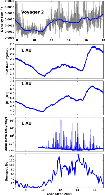
Figure 1. Voyager 2 density (top panel), solar wind ram pressure (second panel), and magnetic field strength at 1 au (third panel) near Earth from OMNI data (King & Papitashvili 2005); the dose rates of solar energetic particles and cosmic rays from the Cosmic Ray Telescope for the Effects of Radiation (CRaTER; Spence et al. 2010; Schwadron et al. 2012; fourth panel) on LRO; and solar sunspot numbers (Svalgaard & Schatten 2016; fifth panel). The abrupt increases in dose rate observed by CRaTER correspond to solar energetic particle events and observed flux ropes associated with solar flares and subsequent coronal mass ejections (Gopalswamy et al. 2014) that propagate out through the heliosphere and drive compressions in the inner heliosheath.
Download figure:
Standard image High-resolution imageIn the fourth panel of Figure 1, we show the dose rate observed by the Cosmic Ray Telescope for the Effects of Radiation (CRaTER; Spence et al. 2010; Schwadron et al. 2012) on the Lunar Reconnaissance Orbiter (LRO), and in the fifth panel we show the solar sunspot number, correcting for the transit time (∼1 yr) from 1 au into the inner heliosheath at the position of V2. As detailed by Schwadron & McComas (2017), CRaTER observations clearly show solar energetic particle events as sporadic, abrupt increases in dose rate. These events mark coronal mass ejections that propagate through the heliosphere, merging and forming large-scale compressions in the outer heliosphere and heliosheath.
Solar activity dropped from 2007 to 2010; subsequently, from 2008 to 2011, V2 data show reductions in density (Figure 1). During the rise in solar activity between 2010 and 2012, a strong compression with increasing density is formed in the inner heliosheath observed from 2011 to 2013.
We take the density structure observed at V2 to move outward radially with the plasma. Inside the termination shock, in the supersonic solar wind, we typically assume that the density structure moves outward radially with a characteristic speed given by the average solar wind speed. In the heliosheath, the flow is subsonic. We then take a characteristic radial propagation speed for the density structure of vp ≈ vw + u, where u is the plasma speed and vw is the wave speed (approximately given by the sound speed).
For the inner heliosheath plasma speed, we use an estimate based on the mass-loading model employed by Schwadron et al. (2014) and Schwadron & McComas (2017). The model based on Isenberg (1987) applies conditions near 1 au and integrates the solar wind plasma properties out through the heliosphere as new pick-up ions created from interstellar neutral atoms mass load the solar wind. The effect of mass loading reduces the solar wind speed with increasing distance from the Sun. Here, we apply the mass-loading model, assuming a solar wind particle flux at 1 au of 3.5 × 108 cm−2 s−1, a solar wind speed at 1 au of 420 km s−1, and a neutral hydrogen density of 0.09 cm−3.
We find an average flow speed u ∼ 100 km s−1 in the inner heliosheath. In addition, based on the downstream properties (downstream density of ∼5 × 10⁻³ cm−3 and downstream internal plasma pressure of ∼2 × 10⁻¹² dyne cm−3 based on the mass-loading model), we take a wave speed vw ∼ 200 km s−1 given approximately by the sound speed. The radial characteristic equation is

Therefore,

Using Equation (7) and Equation (9), we find an average divergence of the plasma flow, given by

Figure 2 shows the total cooling rate (bottom panel) based on Equation (3), which is the sum of the rate due to plasma divergence and the charge-exchange rate (middle panel). The top panel shows the ratio of the flow divergence rate to the charge-exchange rate, τcx/τflow. The yellow-shaded regions in the top panel show when the flow divergence rate exceeds the charge-exchange rate. The flow divergence rate dominates the cooling rate over more than 70% of the time period studied. The longest interval over which the flow divergence rate is smaller than the charge-exchange rate is nine months, from 2013.98 to 2014.72.
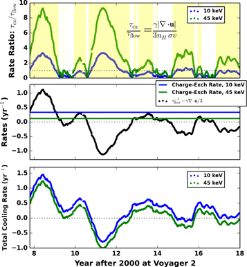
Figure 2. Total cooling rate (bottom panel) based on Equation (3) representing the sum of the rate due to plasma divergence  and the charge exchange rate
  , as shown in the middle panel. The top panel shows the ratio of the flow divergence rate to the charge exchange rate τcx/τflow. The yellow shaded region regions in the top panel show the periods in which the flow divergence rate exceeds the charge exchange rate. The flow divergence rate exceeds the charge exchange for more than 70% of the period shown.
Download figure:
Standard image High-resolution imageFigure 3 shows the cooling timescale from Equation (3) using the average plasma divergence from Equation (10) and an average slope of the distribution γ = 9.5 based on INCA observations. We use the 1 yr averaged density to form the plasma divergence used in the cooling scale. The cooling scale length is defined as λcool = uτcool. Typically, the cooling timescale (Equation (3)) is positive owing to both plasma expansion and charge exchange. However, in the presence of strong plasma compression, the energetic particle distributions are heated, and we define a heating length scale that is opposite to the cooling length scale, λheat = −λcool.

Figure 3. Cooling scale length (middle panel) and cooling timescale (middle panel, scale on right) shown here are derived from the Voyager 2 density. The top panel shows the heating scale length and heating timescale, which is the opposite from the cooling timescale τheat = −τcool and becomes large in the presence of strong plasma compressions. We include in the bottom panel the sunspot numbers for context (see also Figure 1).
Download figure:
Standard image High-resolution image
Figure 3 shows the plasma cooling and heating timescales and length scales over time. We observe rapid plasma cooling or rapid plasma heating in the presence of large-scale expansion or compression of the plasma in the heliosheath. In the time frame of 2008–2010 the cooling timescale is typically reduced to <1–2 yr, whereas in the time frame of (2011–2012), the heating timescale is ∼1 yr.
The effect of heating and cooling in the plasma leads to rapid changes in the particle distribution function, and therefore the ENA flux. In the presence of heating, the distribution function and ENA flux increase with time in the frame of reference of the plasma. However, in the presence of cooling, the ENA flux decreases with time in the frame of reference of the plasma. Therefore, the cooling scale length characterizes the the distance scale over which the distribution decreases beyond the termination shock, whereas the heating scale length characterizes the distance scale over which the distribution increases beyond the termination shock. In Figures 2 and 3, we observe that the plasma is almost always (>70% of the time) driven by time variations, typically over 1–2 year timescales.
The scale length associated with proton charge exchange alone is given by λcx = τcxu. Taking a plasma speed in the heliosheath u ∼ 100 km s−1 and a neutral hydrogen density of 0.09 cm−3, we find a charge exchange length of 62 au at 10 keV and 200 au at 45 keV. From Figure 3, we observe that the cooling scale length (or heating scale length) rarely approaches the charge exchange scale. During plasma expansion, the spatial scales over which energetic particle distributions can be typically observed correspond to ∼20–100 au, based on the full cooling length λcool = u τcool that includes both the effects of loss through charge exchange and adiabatic cooling (see Equation (3)). While plasma compression leads to the buildup of plasma along the line of sight, we find that compression continues over periods of less than 2 years. As a result, the inner heliosheath distributions at INCA energies is almost always (>70% of the time) driven by plasma divergence (compression or expansion). Thus, rapid time variations observed by INCA (Dialynas et al. 2017) are an expected result of plasma divergence in the inner heliosheath and do not place a limit on the size of the heliosheath.
3. Heliosheath Reservoir of Suprathermal and Energetic Particles
The suprathermal and energetic particle distributions observed by IBEX, INCA, and the V2 spacecraft interact over large spatial scales, constituting a suprathermal and energetic particle reservoir. We note from Figure 3 that the cooling scale length (or heating scale length) and cooling time (or heating timescale) become quite similar at 10 and 45 keV over periods of rapid plasma expansion or contraction. This, along with the coordinating changes driven by solar wind, suggests that the energetic particle fluxes will evolve over time in a similar manner over disparate energy ranges.
Energetic particles diffuse typically over large spatial scales. At 1 au, particles in the 10–45 keV energy range typically have scattering mean free paths in the range 0.1–0.5 au (Bieber et al. 1994). Given that the scattering mean free path scales approximately with the inverse of the magnetic field strength, this suggests that the scattering mean free path in the heliosheath will be λ ∼ 10–50 au. Over a given timescale τ, energetic particles diffuse along the magnetic field over a scale length  , where κ∥ = λv/3 and v is the particle speed. Taking a characteristic value of λ = 20 au in the heliosheath, we find that over the cooling timescale of τ ∼ 2 yr, particles diffuse a characteristic distance of D ∼ 60 au at 10 keV and D ∼ 90 au at 45 keV. With a characteristic value of κ⊥/κ∥ = 0.05 (Giacalone & Jokipii 1999), we find a diffusion scale D⊥ ∼ 14 au at 10 keV and D⊥ ∼ 20 au at 45 keV. The diffusion scale lengths are quite large, similar to the width of the heliosheath itself.
Collective behavior from energetic particles also arises from the fact that large-scale compressions and expansions in the heliosheath are well organized by the solar wind. Sokółet al. (2015) reconstructed the spatial and temporal structures of the solar wind from 1985 to 2013 using a combination of in situ and remote-sensing data from observations of interplanetary scintillation (IPS). While some variation is observed over latitude owing to variation between fast and slow solar wind, the density, solar wind flux, and ram pressure show coordination across latitude organized largely by the solar cycle. As a result, we expect large regions of the heliosheath to respond collectively to ram pressure variation driven by the solar wind. Therefore, the response of cooling to heliosheath expansion or the response of heating to heliosheath compression is collective over large regions in the heliosheath (e.g., over the nose and tail regions). In other words, energetic particle distributions at disparate locations will rise and fall in unison as they respond to cooling and heating imparted by expansion or compression of the heliosheath plasma, which is observed by Dialynas et al. (2017). The heliosheath can be thought of as a reservoir of energetic particles, responding collectively over large reions to changes in the background medium of heliosheath plasma.
There are limits to the collective response of energetic particles. For example, the nose and tail regions of the heliosphere are expected to respond differently to plasma compressions and expressions. A propagation delay is expected because the termination shock near the tail is further from the Sun than it is near the nose Schwadron et al. (2014). Furthermore, the different heliosheath geometry near the nose and tail are known to modify how these structures vary in response to changes within the solar wind. The bottom line is that while we expect that energetic particles to respond collectively over large regions, we do not expect that this collective response leads to identical time evolution of energetic particles across the entire heliosheath.
Another factor that arises from the collective response of energetic particles to changes in the heliosheath is the difference in timescales associated with local compressions or expansions versus those that occur across the heliosheath. The cooling and heating scales represented in Figure 2 are local to the plasma at the locations of the V2 spacecraft. As these disturbances propagate through the heliosheath, the energetic particles respond over distance scales comparable to the size of the heliosheath. This leads to a lag in time between the observation of a local compression or rarefaction at V2 and the response from energetic particles across the heliosheath reservoir. Schwadron & McComas (2017) showed that pressure disturbances typically require ∼0.5 yr to propagate from the termination shock to the heliopause in the region near the nose (along the direction of V1). Disturbances within the heliosheath propagate in both directions (sunward and antisunward) owing to the large wave speeds in the heliosheath. As a result, a compressive variation partially reflects at the heliopause and moves back toward the termination shock, which further lengthens the lag time. Using the estimate of wave and plasma speeds indicated previously (wave speed of vw ∼ 200 km s−1 and a plasma speed of u ∼ 100 km s−1), we find a ∼0.5 yr propagation time over 30 au forward through the heliosheath, and a propagation time of ∼1.4 yr of the wave back through the heliosheath to the termination shock. Together this suggests that a disturbance manifests globally within the heliosheath near the nose over a >2 yr timescale.
At the location of V2, a period of plasma expansion and cooling ends roughly at 2010.7 (Figure 2), followed by a period of plasma compression and heating from 2011 through 2013. Given a >2 yr lag time associated with the propagation of local disturbances through the heliosheath, we expect that cooling effects in energetic particles should occur through at least 2012.7. This timeline for expansion/cooling ending late in 2012 followed by a several year phase of compression/heating is roughly consistent with V2 observations; a minimum in energetic particle fluxes (28–43 keV) is observed at V2 at the end of 2012, followed by more than 2 yr of increasing energetic particle fluxes (Dialynas et al. 2017).
We conclude from this discussion that the INCA observations reveal the effects of episodic cooling and heating due to plasma expansion and compression. The large mobility and long diffusive lengths (∼60–90 au along the magnetic field) of energetic protons over the energy range measured by INCA lead to a collective response to large-scale plasma compressions and expansions that occur across the inner heliosheath.
4. Conclusions
Recent energetic neutral atom imaging observations from IBEX and Cassini/INCA have shown rapid 2–3 yr decline and recovery of ENA fluxes. The changes in ENA fluxes observed by INCA are also consistent with the evolution of energetic particle fluxes observed by Voyager 1 and Voyager 2. We show that the cooling (or heating) scale lengths and timescales associated with plasma expansion and compression in the heliosheath are compatible with the rapid changes observed by the Voyagers and Cassini/INCA.
The combination of large diffusive scale lengths (typically 60–90 au along the magnetic field at 10–45 keV) and global effects of expansion and compression in the heliosheath driven by the solar wind causes a collective response over large regions, such as the nose and tail, for energetic particle fluxes over the 2–3 yr timescale changes observed by Voyager and Cassini/INCA. As a result, energetic particle fluxes are expected to change in unison from large regions, such as the nose, as they respond to global compression and expansion in the heliosheath.
We return to the issue raised in the introduction: do the rapid 2–3 yr declines and recoveries in suprathermal and energetic particle ENA fluxes place an observational limit on the size of the heliosphere? The short answer is no. Plasma expansion and compression in the heliosheath have a large influence on the timescale associated with cooling (or heating) of the heliosheath plasma. There is no contradiction between the observation by Cassini/INCA of rapid 2–3 yr decline and recovery of ENA fluxes (10–45 keV; Dialynas et al. 2017) and the evidence of large-scale heliospheric structure (e.g., Zirnstein et al. 2016a), which includes evidence of a heliospheric tail (e.g., McComas et al. 2013).
We are very grateful to the many individuals who have made the the Voyager, IBEX, and Cassini/INCA projects possible. M.B. was supported by Polish National Science Center grant 2015/19/B/ST9/01328.