


Abstract
We publish a photometric redshift catalog based on imaging data of the South Galactic Cap u-band Sky Survey, Sloan Digital Sky Survey (SDSS), and Wide-field Infrared Survey Explorer. A total of seven photometric bands are used, ranging from near-ultraviolet to near-infrared. A local linear regression method is adopted to estimate the photometric redshift with a dedicated spectroscopic training set. The photometric redshift catalog contains about 23.1 million galaxies classified by SDSS. Using the training set with redshift up to 0.8 and r-band magnitude down to 22 mag, we achieve an average bias of  , a standard deviation of σ(Δznorm) = 0.019, and a 3σ outlier rate of about 4.2%. The bias is less than 0.01 at z < 0.6 and goes up to about 0.05 at z ∼ 0.8. Compared with SDSS photometric redshifts, our redshift estimations are more accurate and have less bias.
Export citation and abstract BibTeX RIS
1. Introduction
Redshift is a key factor in studying galaxy evolution, where large redshift samples are needed. Spectroscopic redshift is expensive and time consuming to obtain, while photometric redshift that relies on observed colors is much easier to derive, but less accurate. Over the past decades, the volume of multiwavelength photometric data increased rapidly, as a number of wide or deep imaging surveys have been carried out, such as ESO Imaging Survey (EIS; Nonino et al. 1999), Sloan Digital Sky Survey (SDSS; York et al. 2000), Great Observatories Origins Deep Survey (GOODS; Giavalisco et al. 2004), Galaxy Evolution Explorer (Martin et al. 2005), Canada–France–Hawaii Telescope Legacy Survey (CFHTLS; Ilbert et al. 2006), Two Micron All Sky Survey (Skrutskie et al. 2006), Cosmic Evolution Survey (Scoville et al. 2007b), UKIRT Infrared Deep Sky Survey (Lawrence et al. 2007), Wide-field Infrared Survey Explorer (WISE; Wright et al. 2010), Cosmic Assembly Near-infrared Deep Extragalactic Legacy Survey (Grogin et al. 2011), VISTA Deep Extragalactic Observations survey (Jarvis et al. 2013), Pan-STARRS1 Surveys (PANSTARRS; Chambers et al. 2016), and Dark Energy Survey (DES; Dark Energy Survey Collaboration et al. 2016). The future Large Synoptic Survey Telescope (LSST; LSST Science Collaboration et al. 2009), producing the deepest and widest image of the universe, will allow astronomers to extract a huge sample of galaxies extending to the high-redshift universe. Photometric redshift can be an essential and effective tool to derive well-defined galaxy samples at different cosmic epochs. Now photometric redshifts have been widely used in studying galaxy clusters (Wang & Steinhardt 1998; Heinis et al. 2007; Wen et al. 2012), galaxy evolution (Fontana et al. 2000; Arnouts et al. 2007), large-scale structure (Mazure et al. 2007; Scoville et al. 2007a), and dark energy (Dark Energy Survey Collaboration et al. 2016).
There are two main methods to estimate photometric redshifts. One is the template-matching technique, which requires a set of template spectral energy distributions (SEDs) covering various types of galaxies. Photometric redshifts can be estimated by minimizing χ2 of the difference between observed and template SEDs. Some popular codes based on the template-matching method are HyperZ (Bolzonella et al. 2000), EAZY (Brammer et al. 2008), BPZ (Benítez 2000), and LePhare (Ilbert et al. 2009). The other is the empirical or training approach. Basically, the empirical method is to derive a parameterized relation between redshift and photometric parameters (e.g., colors) with a training set. This training set should be a representative sample of galaxies with accurate photometric parameters and known redshifts. Some representative codes are ANNZ (Firth et al. 2003; Collister & Lahav 2004; Sadeh et al. 2016), MLPQNA (Brescia et al. 2009), Random Forest (Carliles et al. 2010), TPZ (Carrasco Kind & Brunner 2013), GAZ (Hogan et al. 2015), SOM (Masters et al. 2015), and GPZ (Almosallam et al. 2016).
In the presence of consistent and homogeneous spectroscopic coverage in the training set, using empirical methods can improve the photometric redshift accuracy (Hildebrandt et al. 2010; Gieseke et al. 2011). On the other hand, applying more photometric bands with the same training set can also improve the performance of photometric redshift (Capak et al. 2007; Budavári & Szalay 2008; Brescia et al. 2013). Beck et al. (2016) used an empirical method to estimate the photometric redshifts for galaxies in SDSS Data Release 12 (SDSS DR12; Alam et al. 2015). It is reported that the redshift accuracy can reach about 0.021. Based on multiband data from SCUSS, SDSS, and WISE (Wright et al. 2010), we plan to use the same method as in Beck et al. (2016) to produce a photometric redshift catalog and then to identify a sample of galaxy clusters and statistically study their properties and evolution. SCUSS is a u-band imaging survey using the 2.3 m Bok telescope. The survey provides wide-field and deep near-ultraviolet images for an area of more than 4000 deg2 in the south Galactic cap. The 5σ depth for the PSF magnitude is 23.2 mag, which is 1.2 mag deeper than the SDSS u band. Deep SCUSS u and WISE infrared data are useful to accurately estimate photometric redshifts and are also critical for star formation, dust content, and stellar population properties of galaxies.
As the first of a series of papers, we provide a new photometric redshift catalog based on SCUSS, SDSS, and WISE surveys. The organization of this paper is as follows. Section 2 describes the photometric and spectroscopic data. The method to estimate photometric redshift and the description of training data are presented in Section 3. Section 4 gives the accuracy of our photometric redshifts and some comparisons with other catalogs. Section 5 describes the photometric redshift catalog. Section 6 is the conclusion.
2. Data Description
2.1. Photometric Data
The multiband photometric data come from three independent surveys: SCUSS, SDSS, and WISE. The adopted filters are SCUSS u, SDSS ugriz, and WISE W1 and W2. The wavelength coverage ranges from near-ultraviolet to near-infrared (3500 Å–4.6 μm). We describe each survey as below.
SCUSS: SCUSS is a deep u-band imaging survey in the south Galactic cap using the 2.3 m Bok telescope. The telescope is equipped with four 4k × 4k CCDs, which are optimized for the ultraviolet response. The adopted filter is similar to the SDSS u band but slightly bluer and narrower. The survey observations were completed at the end of 2013, covering an area of about 5000 deg2. The data release was published in 2015 December. The data products contain calibrated single-epoch images, stacked images, and photometric catalogs. The area covered by the catalogs is about 4000 deg2. Figure 1 shows the sky coverage of the SCUSS data. About 75% of the area is covered by SDSS (Zou et al. 2016). The median magnitude limit (5σ point sources) is about 23.2 mag. The catalogs contain coadded magnitude measurements on single-epoch images. These measurements are automatic, aperture, PSF, and model magnitudes for both SCUSS unique objects and SDSS sources. The model photometry is consistent with SDSS, which utilizes SDSS r-band model shape parameters to measure brightnesses on SCUSS images (Zou et al. 2015).
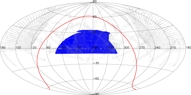
Figure 1. Sky coverage of SCUSS catalogs (blue) in Aitoff projection centered at (0, 0). The red solid curve represents the Galactic plane. The SDSS imaging runs are overplotted in gray.
Download figure:
Standard image High-resolution imageSDSS: SDSS (York et al. 2000) is an influential survey in the world that can implement both imaging and spectroscopic observations by using a dedicated 2.5 m wide-field telescope at Apache Point Observatory. The final imaging survey covers about 14,000 deg2. Most area in the south Galactic cap has been covered after SDSS DR7. SDSS uses a wide-field camera that is made up of 30 CCDs. The imaging observations were taken simultaneously with five broad bands. The magnitude limit with 95% completeness are 22.0, 22.2, 22.2, 21.3, and 20.5 mag for u, g, r, i, and z, respectively. The photometric catalogs contain a number of magnitude measurements, such as Model, cModel, Petrosian, and PSF. The "modelMag" in the SDSS catalog can give unbiased colors of galaxies. It is calculated by applying the r-band galaxy model to other filters.
WISE: WISE is an infrared-wavelength astronomical space telescope launched in 2009. It has performed an all-sky imaging surveys in 3.4, 4.6, 12, and 22 μm, known as W1, W2, W3, and W4, respectively. After 10 months of observations, the telescope depleted the coolant. A new mission called NEOWISE was conducted to search for near-Earth objects with W1 and W2 bands. The imaging resolution is quite low (about 6''). Thus, official all-sky WISE catalogs cannot match the SCUSS/SDSS data, as a large number of sources are lost. The unWISE uses a "forced photometry" technique to measure model magnitudes of SDSS objects in new coadds of WISE images (Lang 2014; Lang et al. 2016). The unWISE catalogs provide flux measurements of all SDSS sources in each WISE band.
In order to estimate photometric redshifts in this paper, the model magnitudes are adopted for all three surveys, since the forced photometry method measures a consistent set of sources between SDSS and SCUSS/WISE and it provides unbiased colors of galaxies. The angular resolutions for WISE W1, W2, W3, and W4 are 6 1, 64, 65, and 120, respectively. The 5σ point-source sensitivities are better than 0.08, 0.11, 1, and 6 mJy for these four bands (Wright et al. 2010). In addition, the unWISE W1 and W2 photometry makes use of new full-depth coadds of the WISE and NOEWISE-reaction images (Lang 2014) and less than 3% of objects in the W3 and W4 bands have photometric S/Ns larger than 5 in unWISE catalogs. Thus, we only use W1 and W2 bands considering low imaging resolution and much shallower photometry in W3 and W4. The SDSS photometric data in this paper are from Data Releases 10 (DR10; Ahn et al. 2014). To avoid confusion, we mark SCUSS u band as u*. Table 1 lists the information of all filters in SCUSS, SDSS, and WISE. The magnitude limits are estimated as 5σ depths of model magnitudes. All magnitudes in this paper are in the AB magnitude system. They are corrected with the Galactic extinction using the reddening map of Schlegel et al. (1998). From Table 1, we can see that the SCUSS u band is about 1.1 mag deeper than the SDSS u band. The last column in this table gives the percentage of galaxies classified by SDSS with S/Ns larger than 5 for each filter. The SCUSS u-band objects with S/N > 5 are twice more than those of SDSS. In addition to u band, the SDSS z and WISE W2 are relatively shallower.
Table 1. Information of All Filters Used in This Paper
| Filter | Effective Wavelength | FWHM | Magnitude Limita | Fractionb |
|---|---|---|---|---|
| (Å) | (Å) | (mag) | ||
| u* | 3538 | 520 | 22.5 | 12.1% |
| u | 3543 | 650 | 21.4 | 5.2% |
| g | 4770 | 1490 | 22.7 | 45.2% |
| r | 6231 | 1440 | 22.3 | 70.4% |
| i | 7625 | 1330 | 21.8 | 75.6% |
| z | 9097 | 1370 | 20.3 | 28.0% |
| W1 | 34000 | 6630 | 20.3 | 50.4% |
| W2 | 46000 | 10430 | 19.6 | 21.8% |
Notes.
aMagnitude limits are computed with model magnitudes at S/N = 5 (equivalently at the magnitude error of about 0.21 mag). bFraction of galaxies with S/N > 5.Download table as: ASCIITypeset image
2.2. Spectroscopic Data
The spectroscopic data are used as a training set and for assessing the quality of photometric redshifts in our paper. We collect spectroscopic redshifts from several surveys, including SDSS, 6DF, DEEP2, VIPERS, VVDS, and WiggleZ. Table 2 lists the references for these surveys. The SDSS DR13 is the largest contributor including early main galaxies, luminous red galaxies from the Baryon Oscillation Spectroscopic Survey (BOSS) of SDSS III and Extended Baryon Oscillation Spectroscopic Survey (eBOSS) of SDSS IV, and emission-line galaxies from eBOSS. We only select galaxies with secure spectral redshift measurements by using quality flags in the catalogs. These flags and their adopted values are also presented in Table 2. The photometric and spectroscopic data are cross-matched with a matching radius of 2''. The matched numbers of galaxies are shown in the last column of Table 2.
Table 2. Different Spectroscopic Redshift Surveys
| Survey | Reference | Quality Flaga | Matchedb |
|---|---|---|---|
| SDSS DR13 | Albareti et al. (2017) | zWarning = 0 | 545356 |
| 6DF | Jones et al. (2004), Jones et al. (2009) | Q = 3, 4 | 6261 |
| DEEP2 | Davis et al. (2003), Newman et al. (2013) | ZQUALITY = 3, 4 | 3045 |
| VIPERS | Garilli et al. (2014), Guzzo et al. (2014) | ZFLAG mod 10 = 3, 4 | 44561 |
| VVDS | Le Fèvre et al. (2005), Garilli et al. (2008) | ZFLAGS mod 10 = 3, 4 | 12481 |
| WiggleZ | Drinkwater et al. (2010), Parkinson et al. (2012) | Class mod 10 = 3, 4 | 23864 |
Notes.
aRedshift quality flags and adopted values in different redshift catalogs. bNumber of galaxies matched with the photometric data.Download table as: ASCIITypeset image
Figure 2 shows the distributions of galaxies with spectroscopic redshifts in both color–color diagram and redshift histogram. Combining spectra from different surveys can improve the completeness of our spectroscopic training set. However, these spectroscopic data are not representative of the full photometric data, so we apply a series of magnitude error and color cuts in Section 3.2 for spectroscopic data to constrain their applicative scope.
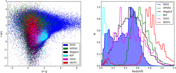
Figure 2. Left: distributions of galaxies with spectroscopic redshifts from different surveys in a color–color diagram of (u* − g ) vs. (r − W1). Right: redshift distributions of the same galaxies. The histograms are normalized to their maximums.
Download figure:
Standard image High-resolution image3. Estimating Photometric Redshift
3.1. Local Linear Regression Algorithm
The local linear regression algorithm has been used for photometric redshift estimation in SDSS DR12 (Beck et al. 2016). The basic idea is to use a linear model to describe the relation between redshift and observed colors in the local color space for each target galaxy whose redshift is to be determined. Since the model magnitudes we used are based on the SDSS r-band shape parameters, the r band is regarded as a fiducial. Assuming a target galaxy with magnitudes of (u*, g, r, i, z, W1, W2), we use a vector  = (u* − r, g − r, r, r − i, r − z, r − W1, r − W2) to express the photometric SED of the galaxy. The local linear model is formulated as:

where c is a constant intercept,  are the linear coefficients, zphot is the photometric redshift to be estimated, and zspec is the spectroscopic redshift. The basic assumption is that galaxies with similar observed SEDs share the same relation. To estimate the photometric redshift for the target galaxy, we need first to find its nearest neighbors with known spectroscopic redshifts in the color space and then derive the regression coefficients in Equation (1) for these neighbors. The redshift of the target galaxy can be finally determined by filling its SED in this equation.
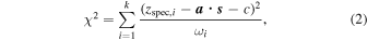
For this local linear regression algorithm, a training set of galaxies with spectroscopic redshifts are required. In addition, the number of nearest neighbors (k) is also a critical parameter. A value that is too large will destroy the locality of the linear model and, meanwhile, will cost a great deal of computing time. Conversely, a value of k that is too small hardly constrains the linear model. After a test of different values, we set k = 50. For larger k, it improves the redshift estimation performance very little but increases the computing time substantially. The nearest galaxies are selected according to the Euclidean distance to the target galaxy in high dimensional color space. After finding the k nearest neighbors, the model is fitted by minimizing χ2 , which is expressed as:
where ωi is the weight. The k nearest galaxies are treated equally in this paper, so we set ωi = 1.
The redshifts of the k galaxies are supposed to be approximate, since they have similar colors. However, sometimes there are outliers whose redshifts obviously deviate from other neighbors. It might be caused by large photometric errors or color-redshift degeneracy. We use the redshift residual of the linear regression model to remove outliers. The residual δz is the same as that used in Beck et al. (2016), which is expressed as:
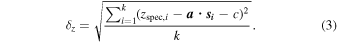
Galaxies with  are removed and the linear model are fitted iteratively. The photometric redshift is calculated using the final model. Following Beck et al. (2016), we use δz as the error estimation of the photometric redshift. The probability density distribution of (zphot − zspec)/δz is similar to a standard normal distribution despite a slight overall bias and more extended wings (see Figure 3). It indicates that δz gives a fair assessment of the photometric redshift error.
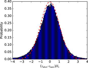
Figure 3. Normalized distribution of (zphot − zspec)/δz. The red dashed curve is a standard normal distribution.
Download figure:
Standard image High-resolution image3.2. Training Set
As described above, a robust training set with known spectroscopic redshifts is required to obtain a reliable local linear regression model. The galaxies with large photometric errors can have influence on the determination of nearest neighbors. We need to introduce photometric error cuts. Besides, color cuts are also needed to exclude galaxies with erroneous color measurements and unusual colors. These error and color cuts are decided empirically and are listed as below:
The cut for r-band magnitude error (Δr) is set to 0.15, which is also adopted in Beck et al. (2016) to remove galaxies with photometric errors that are too large. About 95% of galaxies with spectroscopic redshifts have Δr < 0.15. The error cuts for other colors follow the same fraction. There is no constraint on (u − r) due to large photometric errors of redshifted galaxies at u band. As shown in Equation (4), the error cuts for (g − r) are relatively larger. Our galaxies have median spectroscopic redshift of about 0.4. As the redshift goes up to 0.5, the Balmer break shifts to 6000 Å. Correspondingly, the g-band photometric error increases. The (r − z) and (r − W2) error cuts are also large due to large photometric errors of z and W2 bands. Although these bands have larger photometric errors than other bands, we can still give secure photometric redshifts. The color cuts are set where the highest and lowest 0.5% of galaxies are located. Through both error and color cuts, about 38% of galaxies are removed. The final training set has 396,352 galaxies. Figure 4 shows both r-band magnitude and redshift distributions of galaxies with spectroscopic redshifts before and after those cuts are applied. The r-band magnitude can extend up to about 22.0 mag. After the cuts are applied, the redshift distribution becomes more homogeneous. The redshift extends up to about 0.8.

Figure 4. Left: r-band magnitude distributions of galaxies with spectroscopic redshifts. Right: redshift distributions of these galaxies. Red and blue lines are the distributions before (red) and after (blue) error and color cuts are applied, respectively.
Download figure:
Standard image High-resolution image4. Results and Analyses
4.1. Accuracy of Photometric Redshifts
The filtered training data through both error and color cuts are equally divided into two subsets. One is used as the training set for deriving the local linear regression model and the other is used as the testing set for accuracy estimation of the photometric redshift. The normalized redshift error presented in Beck et al. (2016) is defined as  . With the testing set, we achieve an average bias of
  and a standard deviation of σ(Δznorm) = 0.019. These values are calculated with an outlier rate of Po = 4.2%, where galaxies are removed iteratively using a 3σ clipping algorithm. The left of Figure 5 shows a comparison between spectroscopic and photometric redshifts of galaxies in the testing set. About 92.7% of galaxies are located in
  . The middle and right panels of Figure 5 present Δznorm as a function of the photometric and spectroscopic redshifts. The 1σ error of Δznorm as a function of zspec or zphot is also overplotted. We can see that the photometric redshift can reach up to 0.6, which is limited by our training set. The bias of Δznorm is less than 0.01 and σ(Δznorm) is less than 0.03 at zspec < 0.6. For galaxies with redshifts zspec > 0.6, the photometric redshifts tend to be underestimated mainly due to a lack of high-z galaxies in the training set. We provide a comparison of redshift distributions of the nearest neighbors for galaxies at zspec = 0.3 and zspec = 0.7 in Figure 6. In contrast to zspec = 0.3 galaxies, the galaxies at zspec = 0.7 have their nearest neighbors locating at lower redshifts, so that more neighbors with lower redshifts are involved in the redshift estimations and thus the photometric redshift is underestimated.

Figure 5. Left: zphot as a function of zspec for galaxies in the testing set. The green dashed line is for zphot = zspec, and red dashed lines are for Δznorm = ± 0.05. Middle: Δznorm as a function of zphot. Right: Δznorm as a function of zspec. The red solid and dashed lines represent the median and 1σ standard deviation of Δznorm. The green dashed lines show Δznorm = 0. The density of galaxies is plotted in grayscale.
Download figure:
Standard image High-resolution image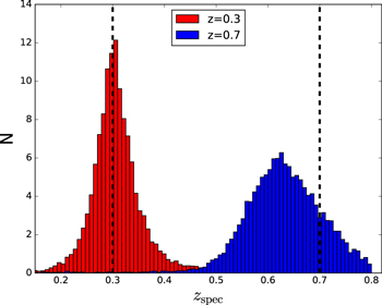
Figure 6. Redshift distributions of nearest neighbors for galaxies at z = 0.3 (red) and z = 0.7 (blue). Two dashed vertical lines give the positions of z = 0.3 and z = 0.7.
Download figure:
Standard image High-resolution imageFigure 7 shows Δznorm as a function of r-band magnitude based on spectroscopic data within color cuts but without error cuts. From this figure, we can see that the photometric redshift error increases with magnitude (or photometric error). Photometric errors strongly limit the accuracy of photometric redshifts. Large photometric errors may lead observed colors of galaxies deviating from true ones and thus affect the finding of nearest neighbors. The redshift bias is less than 0.01 for galaxies with r < 21.5 and can be up to 0.03 at r = 22. The 1σ error is less than 0.04 for galaxies with r < 21 and can be up to about 0.08 at r = 22. In addition to the photometric error, the color-redshift degeneracy can also affect the photometric redshift accuracy. The nearest neighbors with similar colors might have distinct redshifts. In this case, the estimated redshift is likely to be catastrophic.
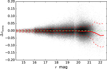
Figure 7. Δznorm as a function of the r-band magnitude. Red solid and dashed lines represent the median and standard deviation with outliers removed by 3σ clipping. The green dashed horizontal line shows zphot = zspec. The number density of galaxies is plotted in grayscale.
Download figure:
Standard image High-resolution image4.2. Comparing with Photometric Redshifts of CFHTLS and SDSS
The CFHTLS provides publicly available photometric redshifts in four wide fields (Ilbert et al. 2006; Coupon et al. 2009). These four fields cover about 155 deg2 with SDSS-like filters. The mean r-band magnitude limit for 80% completeness of point-like sources is about 25.0 mag. The catalogs of Coupon et al. (2009) provide photometric redshifts for galaxies with i < 24. We choose one of the four wide fields (hereafter CFHTLS-W1) to compare with our photometric redshifts. The CFHTLS-W1 is located at (α = 34 5, δ = − 7°). Most of the area is covered by SCUSS. The CFHTLS-W1 photometric redshifts are calibrated by spectroscopic redshifts, giving a standard deviation of σ(Δznorm) ∼ 0.037. We also check that there are no biases in CFHTLS-W1 photometric redshifts using our spectroscopic training set, which is shown in Figure 8(a). The CFHTLS provides a deep photometric redshift catalog, while SDSS provides a wide one. We obtain the photometric redshifts for galaxies in the CFWHLS-W1 field from SDSS DR12 (Beck et al. 2016).
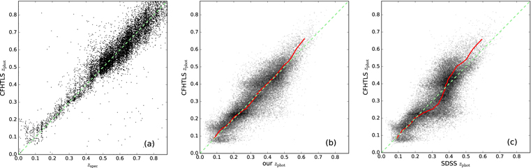
Figure 8. (a) CFHTLS zphot vs. zspec for galaxies with spectroscopic redshifts located in the CFHTLS W1 field. (b) Comparison of our and CFHTLS photometric redshifts. (c) Comparison of SDSS and CFHTLS photometric redshifts. The green dashed lines show the diagonal of x = y. The red solid lines give the median distributions of galaxies. The density of galaxies is plotted in grayscale.
Download figure:
Standard image High-resolution imageBased on the CFHTLS catalog, the comparison of our and SDSS photometric redshifts are shown in Figures 8(b) and (c). We only selected the galaxies with photoErrorClass = 1 in the SDSS photometric redshift catalog, which are regarded to have best redshift estimations as claimed in Beck et al. (2016). There are about 63,000 galaxies in total. From these plots, we can see that the photometric redshifts from three catalogs are in good agreement for galaxies with z < 0.2. However, the SDSS photometric redshift has serious bias at redshift z > 0.2. The redshift is overestimated at 0.2 < z < 0.4 and underestimated at z > 0.4. The bias can reach up to 0.05. Our photometric redshifts give much smaller bias relative to CFHTLS at z < 0.5.
4.3. Effect of SCUSS u and WISE Bands
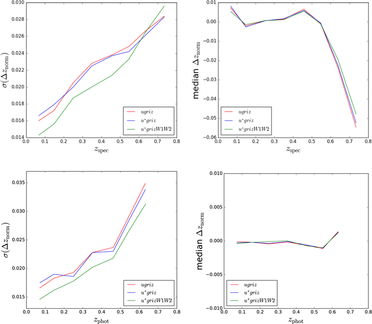
Usually more photometric bands with appropriate depths give better photometric redshift estimations. Compared with SDSS photometric redshifts, we add deep SCUSS u and two WISE infrared bands. To investigate the effect of SCUSS and WISE data on the photometric redshift estimation, three sets of filters are tested by our redshift estimating method using the same training set. One set is ugriz only from SDSS and the other two are u*griz and u*grizW1W2 from SCUSS, SDSS, and WISE. The top panels of Figure 9 show σ(Δznorm) and biases (median Δznorm) as functions of the spectroscopic redshift for these different filter sets. In these plots, we can see that the bias for the three filter sets performs similarly and the redshift is underestimated at z > 0.6. The photometric redshift accuracy of σ(Δznorm) is slightly improved by replacing the SDSS u band with SCUSS u* at z > 0.2. Although the improvement is less obvious, SCUSS can provide twice more galaxies within the same S/N limit as illustrated in Table 1. After adding infrared W1 and W2 bands, the photometric redshift accuracy is significantly improved, especially for galaxies of z < 0.6. We also show σ(Δznorm) and bias as functions of the photometric redshift for the three different filter sets in the bottom panels of Figure 9. The bias is less than 0.2% of the overall redshift range. The σ(Δznorm) at higher zphot is somewhat larger than that at the same zspec due to redshift underestimation of high-z galaxies.
Figure 9. Top left: σ(Δznorm) as a function of the spectroscopic redshift for different filter sets. Top right: median Δznorm as a function of the spectroscopic redshift. Bottom left: σ(Δznorm) as a function of the photometric redshift for different filter sets. Bottom right: median Δznorm as a function of the photometric redshift.
Download figure:
Standard image High-resolution image
5. The Catalog
Our photometric redshift catalog is based on SDSS galaxies with r-band positive model flux measurements. The source type is from the SDSS star/galaxy separation. The photometric redshift accuracy is dependent on the photometric error, number of used filters, and completeness of the training set. In our catalog, we only provide the photometric redshifts for galaxies with r < 22 mag. Meanwhile, we require that at least five colors meet the same color limits for the training set as shown in Equation (4), but no photometric error cut is applied. There are a total of 23,067,608 galaxies with these constraints. The catalog can be accessed though the link http://batc.bao.ac.cn/~zouhu/doku.php?id=projects:photoz:start.
Table 3 lists the information included in our photometric redshift catalog. All magnitudes in this catalog are AB model magnitudes with corrections of the Galactic extinction. The model magnitudes are measured with prior shape parameters from SDSS r band. The magnitude errors for each band are also provided. The SDSS photometric ID and coordinates are kept for conveniently tracing objects in SDSS catalogs. For each object, we provide the photometric redshift from our local linear regression model, average redshift of nearest neighbors in the training set, and redshift of the closest neighbor. The error of the photometric redshift derived by the local linear model is also provided. There is some additional information, such as the number of neighbors used for redshift estimation, number of filters with colors within color cuts, and average Euclidean distance of a galaxy to its neighbors. They are useful for estimating the redshift quality. A small number of neighbors or large Euclidean distance indicate that there are not enough neighbors with similar SEDs to the galaxy. The number of filters that have colors within color cuts is also important for the redshift accuracy. As the number of filters increases, the photometric redshift accuracy becomes better. Table 4 shows the accuracy of our photometric redshift for different numbers of filters. There are about 18.4%, 30.0%, and 51.6% of total objects in our catalog having 5, 6, and 7 filters with colors within color cuts, providing redshift accuracies of about 0.061, 0.028, and 0.019, respectively.
Table 3. Column Description of Our Photometric Redshift Catalog
| Column | Unit | Description |
|---|---|---|
| objID | ⋯ | SDSS photometric object ID |
| n_neighbour | ⋯ | Number of the neighbors used for estimating the photometric redshift |
| n_filter | ⋯ | Number of filters having r < 22 mag and colors within color cuts |
| RA | degree | R.A. in J2000 |
| DEC | degree | Decl. in J2000 |
| spec_z | ⋯ | Spectroscopic redshift if it exists |
| photo_z | ⋯ | Estimated photometric redshift by the local linear regression model |
| photo_zerr | ⋯ | Estimated error for the above redshift |
| photo_zbias | ⋯ | Bias between the photometric and spectroscopic redshifts of the neighbors |
| mean_z | ⋯ | Average spectroscopic redshift of the neighbors |
| nearest_z | ⋯ | Spectroscopic redshift of the nearest neighbor |
| mean_dis | ⋯ | Average Euclidean distance of neighbors in the multidimensional color space |
| scuss_u | mag | SCUSS u-band model magnitude |
| sdss_u | mag | SDSS u-band model magnitude |
| sdss_g | mag | SDSS g-band model magnitude |
| sdss_r | mag | SDSS r-band model magnitude |
| sdss_i | mag | SDSS i-band model magnitude |
| sdss_z | mag | SDSS z-band model magnitude |
| wise_w1 | mag | WISE W1 model magnitude |
| wise_w2 | mag | WISE W2 model magnitude |
| scuss_uerr | mag | SCUSS u-band model magnitude error |
| sdss_uerr | mag | SDSS u-band model magnitude error |
| sdss_gerr | mag | SDSS g-band model magnitude error |
| sdss_rerr | mag | SDSS r-band model magnitude error |
| sdss_ierr | mag | SDSS i-band model magnitude error |
| sdss_zerr | mag | SDSS z-band model magnitude error |
| wise_w1err | mag | WISE W1 model magnitude error |
| wise_w2err | mag | WISE W1 model magnitude error |
Download table as: ASCIITypeset image
Table 4. Photometric Redshift Qualities for Different Numbers of Filters Having Colors within Color Cuts
| n_filtera |

|
σ(Δznorm) | Po | Percentb |
|---|---|---|---|---|
| 7 | −0.0003 | 0.019 | 4.5% | 51.6% |
| 6 | −0.0017 | 0.028 | 6.1% | 30.0% |
| 5 | −0.0072 | 0.061 | 8.7% | 18.4% |
Notes.
aNumber of filters having r < 22 mag and colors within color cuts. bFraction of galaxies in our photometric redshift catalog having specified n_filter.Download table as: ASCIITypeset image
6. Conclusion
Photometric redshift is an important technique to generate a large sample of galaxies at different redshifts. Based on multiwavelength photometric data from SCUSS, SDSS, and WISE surveys, we plan to construct a sample of galaxy clusters to statistically study their properties and the environment effect on galaxy evolution. As the first of a series of work, this paper describes the photometric redshift catalog.
There is a total of seven photometric bands used in the photometric redshift estimation: SCUSS u, SDSS griz, and WISE W1 and W2. The model magnitudes are adopted, which are based on the SDSS r-band shape parameters. They can provide unbiased colors of galaxies. The WISE photometry is not official. It comes from unWISE, which uses new coadds of WISE images and forced photometry. The method to estimate the photometric redshift is the same as that used in Beck et al. (2016). It builds a local linear regression model between observed colors and redshifts from nearest neighbor galaxies within a dedicated spectroscopic training set. The spectroscopic data are from SDSS DR13, 6DF, DEEP2, VIPERS, VVDS, and WiggleZ. The training set is fine-tuned by error and color cuts to remove galaxies with large photometric errors and erroneous colors. The redshift can reach up to about 0.8 and r-band magnitude goes down to about 22 mag.
The photometric redshift catalog includes about 23.1 million galaxies with r < 22 mag and at least 5 filters having colors within the color cuts. The star/galaxy separation is taken from SDSS. Our photometric redshift catalog can be retrieved through the link http://batc.bao.ac.cn/~zouhu/doku.php?id=projects:photoz:start. There are several parameters that can be used for assessing redshift quality: (a) number of nearest neighbors, (b) number of filters with colors within color cuts, (c) redshift error defined as the redshift scatter of the neighbors, and (d) average Euclidean distance from the neighbors.
With the test sample from the training set, we obtain an average bias of  and standard deviation of σ(Δznorm) = 0.019. The redshift accuracy decreases as the magnitude goes fainter. As r > 21.5 mag, the bias is larger than 0.01. In addition, the bias is less than 0.01 as redshift z < 0.6 and goes up to about 0.05 at z ∼ 0.8. By adding SCUSS u and WISE bands to the SDSS photometric data, we can improve the photometric redshift accuracy. Using the photometric redshifts from CFHTLS wide fields as the reference, we have compared the SDSS photometric redshifts. As a result, the SDSS redshift estimation has a large bias at z > 0.2.
This work is supported by the Young Researcher Grant of National Astronomical Observatories, Chinese Academy of Sciences, the Chinese National Natural Science Foundation (grant Nos. 11433005, 11673027, 11733007), the National Basic Research Program of China (973 Program; grant Nos. 2015CB857004, 2014CB845704, 2014CB845702, and 2013CB834902), and the External Cooperation Program of Chinese Academy of Sciences (grant No. 114A11KYSB20160057).
SDSS-III is managed by the Astrophysical Research Consortium for the Participating Institutions of the SDSS-III Collaboration including the University of Arizona, the Brazilian Participation Group, Brookhaven National Laboratory, Carnegie Mellon University, University of Florida, the French Participation Group, the German Participation Group, Harvard University, the Instituto de Astrofisica de Canarias, the Michigan State/Notre Dame/JINA Participation Group, Johns Hopkins University, Lawrence Berkeley National Laboratory, Max Planck Institute for Astrophysics, Max Planck Institute for Extraterrestrial Physics, New Mexico State University, New York University, Ohio State University, Pennsylvania State University, University of Portsmouth, Princeton University, the Spanish Participation Group, University of Tokyo, University of Utah, Vanderbilt University, University of Virginia, University of Washington, and Yale University.
Funding for the DEEP2 Galaxy Redshift Survey has been provided by NSF grants AST-95-09298, AST-0071048, AST-0507428, and AST-0507483 as well as NASA LTSA grant NNG04GC89G. This paper uses data from the VIMOS Public Extragalactic Redshift Survey (VIPERS). VIPERS has been performed using the ESO Very Large Telescope, under the "Large Programme" 182.A-0886. The participating institutions and funding agencies are listed at http://vipers.inaf.it. This research uses data from the VIMOS VLT Deep Survey, obtained from the VVDS database operated by Cesam, Laboratoire d'Astrophysique de Marseille, France. We wish to acknowledge financial support from The Australian Research Council (grants DP0772084, LX0881951, and DP1093738 directly for the WiggleZ project, and grant LE0668442 for programming support), Swinburne University of Technology, The University of Queensland, the Anglo-Australian Observatory, and The Gregg Thompson Dark Energy Travel Fund at UQ.