


Abstract
We present the catalog of ∼31,500 extragalactic H i line sources detected by the completed Arecibo Legacy Fast ALFA (ALFALFA) survey out to z < 0.06, including both high signal-to-noise ratio (>6.5) detections and ones of lower quality that coincide in both position and recessional velocity with galaxies of known redshift. We review the observing technique, data reduction pipeline, and catalog construction process, focusing on details of particular relevance to understanding the catalog's compiled parameters. We further describe and make available the digital H i line spectra associated with the cataloged sources. In addition to the extragalactic H i line detections, we report nine confirmed OH megamasers (OHMs) and 10 OHM candidates at 0.16 < z < 0.22 whose OH line signals are redshifted into the ALFALFA frequency band. Because of complexities in data collection and processing associated with the use of a feed-horn array on a complex single-dish antenna in the terrestrial radio frequency interference environment, we also present a list of suggestions and caveats for consideration by users of the ALFALFA extragalactic catalog for future scientific investigations.
Export citation and abstract BibTeX RIS
1. Introduction
A census of the extragalactic population of atomic gas-bearing galaxies is provided by H i 21 cm line surveys. Because of the relatively simple physics involved in most H i line emission, conversion of the observed line flux into atomic hydrogen gas mass is straightforward, and the spectral nature of the emission provides observable measures of the redshift and projected disk rotational velocity. While the molecular H2 gas tends to concentrate in a small number of giant gas clouds, principally in the inner regions, the H i disk traces the full extent of the gas layer. Star formation is linked more closely to the molecular H2 gas (e.g., Kennicutt & Evans 2012; Saintonge et al. 2016; Catinella et al. 2018). However, in most galaxies, the H i fills a much larger fraction of interstellar space and contributes most of the cool gas mass, thus representing the fuel reservoir and potential for future star formation.
The Arecibo Legacy Fast ALFA (ALFALFA) Survey used the seven-horn Arecibo L-band Feed Array (ALFA) to map nearly 7000 deg2 of high Galactic latitude sky accessible to the Arecibo telescope over ∼4400 nighttime hours between 2005 and 2011. ALFALFA was conducted as a "blind" survey: at each position, the entire frequency range from 1335 to 1435 MHz, corresponding to heliocentric velocities −2000 km s–1 < cz < 18,000  , was searched for line emission. As described in detail by Giovanelli et al. (2005), the ALFALFA survey design was largely dictated by the principal science goal of determining the faint end of the H i mass function (HIMF) and the overall abundance of low-mass gas-rich halos (e.g., Martin et al. 2010, 2012; Papastergis et al. 2011, 2013). Additional objectives include how the HIMF might vary with environment (e.g., Moorman et al. 2014; Jones et al. 2016b, 2018), how the H i–bearing population differs from optically selected ones (e.g., Huang et al. 2012a, 2012b; Gavazzi et al. 2013), using the H i distribution to look for tidal debris on large angular scales (e.g., Lee-Waddell et al. 2014, 2016; Leisman et al. 2016), and establishing metrics for the normal H i content of galaxies (e.g., Toribio et al. 2011; Odekon et al. 2016). As the least-clustered local (z ∼ 0) galaxy population (Martin et al. 2012), the H i–bearing population traces how galaxies evolve when left on their own in relative isolation.
ALFALFA has also discovered a number of enigmatic objects, such as the nearby faint dwarf Leo P (Giovanelli et al. 2013), the very metal-poor Leoncino (Hirschauer et al. 2016), and the highly H i–dominated Coma P (Janowiecki et al. 2015; Ball et al. 2018). Additionally, ALFALFA has provided the opportunity to survey classes of galaxies such as extremely low H i mass dwarfs (e.g., Cannon et al. 2011; McNichols et al. 2016; Teich et al. 2016), galaxies with extremely high H i–to–stellar mass ratios (e.g., Adams et al. 2015b; Janesh et al. 2015, 2017; Janowiecki et al. 2015), and H i–bearing ultra-diffuse galaxies (Leisman et al. 2017). The vast majority (>98%) of extragalactic ALFALFA sources can be associated with at least one likely stellar counterpart, and the majority of the "dark" objects are likely associated with tidal debris in interacting systems (e.g., Haynes et al. 2007; Koopmann et al. 2008; Lee-Waddell et al. 2014; Leisman et al. 2016). A few dark galaxy candidates remain intriguing, and continuing work seeks to identify associated starlight and constrain their dynamics and star formation history (e.g., Giovanelli et al. 2010; Kent 2010; Cannon et al. 2015).
As a complement to Jones et al. (2018), which presents the derived HIMF and its dependence on the local environment, this paper presents the extragalactic H i catalog extracted from the completed ALFALFA survey. Because of the overlapping nature of the drift-scan survey and improved availability of the public optical imaging used to identify optical counterparts (OCs) of ALFALFA H i sources, this catalog, presented in Table 2, supersedes and replaces previous releases (Giovanelli et al. 2007; Kent et al. 2008; Saintonge et al. 2008; Martin et al. 2009; Stierwalt et al. 2009; Haynes et al. 2011). In addition to the catalog of ALFALFA H i line detections, nine sources are identified with OH megamasers (OHMs), and 10 are flagged as being OHM candidates.
Section 2 reviews the important aspects of the ALFALFA survey observational program and data reduction process that has led to the production of the extragalactic data set presented in Section 3. Section 4 summarizes a number of important points, realities, and caveats about the survey and its resultant data products that readers are encouraged to keep in mind. Appendix A presents details of the data acquisition and processing pipeline used to produce the ALFALFA catalog.
To allow direct comparison with the vast majority of extant works on H i line emission at low redshift, we use the observed rest frame and do not apply cosmological corrections dependent on redshift; those amount to at most a few percent for the most distant sources. Details of this choice are given in the text.
2. The ALFALFA Survey
The ALFALFA survey was intended to cover two sky areas at high Galactic latitude, one in the northern Galactic hemisphere, 07h30m < R.A. < 16h30m, 0° < decl. < +36°, and one in the southern hemisphere, 22h < R.A. < 03h, 0° < decl. < +36°. For various practical reasons, the final sky area, depicted here in Figure 1 and also shown in Figure 1 of Jones et al. (2018), is somewhat reduced near the edges.

Figure 1. Sky distribution of ALFALFA sources included in Table 2 in the northern (top) and southern (bottom) Galactic hemispheres, showing the roughness of boundaries imposed by practical and scheduling constraints.
Download figure:
Standard image High-resolution imageAs discussed in Giovanelli et al. (2005) and Giovanelli & Haynes (2015), the ALFALFA survey was designed particularly to sample the HIMF over a fair cosmological distance of ≃100 Mpc, therefore setting minimum requirements on the survey volume sensitivity and areal coverage. For a survey with a telescope characterized by a given system temperature Tsys and gain G, the science-driven need to detect a given H i mass MH i of H i line width W50  at a distance DMpc translates to a required integration time tint in seconds of

where γ ≃ −1/2 for W50 < 200  and −1 for W50 > 200
  (Giovanelli et al. 2005; Giovanelli & Haynes 2015). The ALFALFA HIMF science goal dictates that the survey cover a very wide solid angle, Ωsurvey ∼ 7000 deg2, with an average integration time of ∼48 s per beam solid angle after combination of all drifts from all beams and polarizations across each spatial point. The sheer amount of telescope time (thousands of hours) needed to accomplish such wide sky coverage in turn demanded an observing strategy that exploited Arecibo's large collecting area, the mapping capability of the ALFA instrument, and the spectral power of its back-end spectrometer to maximum observing efficiency.
2.1. Drift-scan Technique
As discussed in detail in Giovanelli et al. (2005), ALFALFA was conducted as a drift-scan survey using the seven feed-horn array ALFA. The ALFA feed-horn configuration delivers a central, higher-gain beam surrounded by a ring of six equally spaced, somewhat lower-gain beams. For most of the survey, the azimuth arm of the telescope was positioned on the meridian at a preassigned J2000.0 decl., with a spacing of 14 6 between primary drift centers. The feed array was rotated by 19° so that the Earth-rotation drift-scan tracks of individual beams were equally spaced by 21 in decl. in J2000.0 coordinates. A second, parallel drift pass of the same region of the sky was acquired later, with the center beam offset from the first by 73 (half the spacing to the next primary center beam positioning) so that the final sampling in decl. was 105. Because hardware limits do not allow pointing straight overhead, coverage of decl. located close to the zenith (decl. = +18° 21') with similar parallel tracks required the telescope to be positioned off-meridian and the array rotated by a different amount, depending on the decl. of the array center. Spectra were acquired covering a 100 MHz bandwidth centered at 1385 MHz using the Wide-band Arecibo Pulsar Processor (WAPP) spectrometer, yielding 4096 "channels" per spectrum, equally spaced in frequency, for each of two linear polarizations of each of the seven feed horns (a total of 14 spectra). Parameters of the ALFALFA observing setup and specifications are summarized in Table 1.
Table 1. ALFALFA Technical Details
| Number of beams | 7 |
| Polarizations per beam | 2 linear |
| Beam size (FWHM) | 38 × 33 |
| Gain | 11 K Jy−1 (central beam) and 8.5 K Jy−1 (peripheral) |
| Tsys | 26–30 K |
| Frequency range | 1335–1435 MHz |
| cz⊙ range | −2000 to 17912  |
| Bandwidth (total) | 100 MHz |
| Correlator lags (spectral channels) | 4096 |
| Channel spacing | 24.4 kHz (5.1  at 1420.4058 MHz) at 1420.4058 MHz) |
| Spectral resolution | 10  , after Hanning smoothing , after Hanning smoothing |
| Autocorrelation sampling | 3 level |
| Avg. channel rms | 2.0 mJy channel−1 |
| Map rms | 1.86 mJy beam−1 |
| Effective map tint | 48 s (beam solid angle)−1 |
| 5σ survey sensitivity | 0.72 Jy  for W50 = 200 for W50 = 200  at tint at tint |
| Single-drift sky coverage | 600 s × 146 (all beams) |
| Drift-scan size on disk | 213 MB |
| Grid sky coverage | 2 4 × 24 4 × 24 |
| Grid center spacing | 8 minutes in R.A. and 2° in decl. |
| Grid cz⊙ coverage | (a) ∼−2000 to 3300  |
(b) ∼2500 to 7950  |
|
(c) ∼7200 to 12,800  |
|
(d) ∼12,100 to 17,912  |
|
| Grid cz overlap | 140 channels |
| Grid size on disk | 381 MB |
Download table as: ASCIITypeset image
The drift-scan observations were conducted in observing runs that typically lasted 4–9 hr at a time, normally without interruption, yielding an exceptionally high efficiency of "open-shutter time." Once data acquisition for an observing run began, 14 individual spectra (polarizations/beams) were recorded each second at 99% time efficiency, except for two adjustments made every 600 s. First, minor pointing corrections were made to maintain the pointing of the ALFA central beam in constant decl. J2000.0 coordinates; it may be noted that this approach insured that adjacent or contiguous drift scans taken several years apart would thus remain parallel in that coordinate frame. The corrections from current epoch to J2000 coordinates depend on source position and, over the 7 yr period of data-taking, amount in some positions to several arcminutes.
In addition to the minor position update, the data acquisition sequence was interrupted every 600 s to allow the injection of a calibration noise diode for 1 s; because of hardware notifications ("hand-shaking"), this procedure, described in more detail in Appendix A, took in practice between 4 and 7 s, still less than the time for a source to cross a single ALFA beam (14 s). No other adjustments were made. This "minimum-intrusion" approach allowed tracking of separate polarization/beam/spectral behavior over a timescale of hours to compensate for systematic variations (e.g., drifts in "electronic gain"). Occasionally, hardware failures led the observing sequence to be aborted. In such cases, power levels were readjusted before data acquisition was restarted. Because of the desire to calibrate using a significant number (at least nine) of calibration samples, drift sequences of less than 90 minutes were discarded. In general, the lack of power readjustment and minimal telescope motion delivered very high overall data quality and robust system calibration.
2.2. Radio Frequency Interference
A major complication of observing the H i 21 cm line in the 1335–1435 MHz range is introduced by the presence of human-generated radio frequency interference (RFI), typically over relatively narrow ranges in frequency occupying a few MHz or substantially less. Some RFI is predictable, some is (nearly) omnipresent, and some is transient. Most RFI is polarized, and some is very strong, causing a rise in the system temperature (Tsys) and sometimes introducing spectral standing waves (due to multiple reflections/scattering within the Arecibo telescope optical path). Mitigation of RFI was addressed in several different ways. To make possible the identification of RFI by statistical differences in power levels, a second drift across each part of the sky was undertaken, typically with the second pass centered halfway between adjacent tracks of the first pass and acquired 3–9 months later than the first. Since Doppler tracking was not implemented, the offset in the time of data acquisition allowed the discrimination of fixed-frequency RFI from cosmic sources. Each spot on the sky was included in multiple drift scans and beams/polarizations, such that a statistical comparison of subsets of data could be checked for inconsistencies caused by bursts of RFI.
The strongest and most persistent (except for a period of a few months for its replacement) RFI feature arises from the FAA radar at the San Juan airport centered near 1350 MHz. The airport radar transmission is pulsed, polarized, azimuth-dependent, and not picked up equally by all beams. When it is strong, harmonics generated within the Arecibo spectral chain may show up at 1380 and (sometimes) 1405 and 1410 MHz. Another common RFI source, evident near 1381 MHz in shorter bursts of 60–180 s at a time, is associated with the NUclear DETonation (NUDET) detection system aboard the global positioning system (GPS) satellites. Many other transient RFI sources were present, arising from spurious transmissions, faulty equipment, etc. In order to address RFI contamination, each individual polarization/beam spectral drift scan was run through an RFI flagging routine and then examined by an expert who could accept or reject the pipelined flags and/or set additional ones. While laborious, this procedure of data flagging produced a spectral mask that maintains a record of flagged spectral pixels, important for identifying RFI "holes" in the 21 cm line sky, as the spectrum at each grid point is associated with a spectral weight at each frequency/velocity point.
Similar to the depictions of the typical spectral weights in previous ALFALFA data release papers, e.g., Figure 1 of Giovanelli et al. (2007) and Figure 6 of Martin et al. (2010), Figure 2 shows the normalized weight per spectral channel derived from the entire set of ALFALFA grids (top panel) and for two different decl. strips of grids covering the northern Galactic ALFALFA regions (bottom panel). The most prominent reduced-weight features reflect contamination by the San Juan airport FAA radar near 1350 MHz (∼15,600  ) and modulations of it at 1380 MHz (∼8800
  ), 1405 MHz (∼3300
  ), and 1410 MHz (∼2200
  ). As found earlier by Giovanelli et al. (2007), on average, about 85% of the total bandpass was RFI-free with a normalized weight >0.9. Of the bandpass, 94% carries a spectral weight of >0.5; that value can serve as an acceptable limit on data quality. Because of the large percentage of channels corrupted by the FAA radar systems at frequencies below 1350 MHz, statistical studies requiring volume completeness should be restricted to galaxies within the corresponding velocity limit of cz < 15,000
  (Martin et al. 2010).

Figure 2. Normalized spectral weight at each of the final (nonoverlapping) 3672 frequency channels displayed in the corresponding velocity units for the entire set of ALFALFA grids (upper) and for two strips of grids across the northern Galactic hemisphere (lower) at decl. = +07° (blue line) and +33° (dashed red line). The main cause of missing data (reduced spectral weight) is RFI, most notably the 1350 MHz (cz ∼ 15,600 km s−1) FAA radar at the San Juan airport. Narrower features at 8800, 3300, and 2200 km s−1 are modulations of the FAA radar occurring within the WAPP spectrometer. Comparison of the panels illustrates the varying nature of the RFI during different observing periods and the serious contamination caused by the 1345–1350 MHz radar system at velocities above 15,000  .
.
Download figure:
Standard image High-resolution imageA more detailed discussion of the drift-scan data acquisition, calibration, processing, and RFI flagging process is presented in Appendix A.
2.3. Grid Production
Upon acquisition of all of the drift scans covering a region of sky, all of the relevant spectra were combined to produce a 3D spectral grid; further details of this process are given in Appendix A.2. In the spatial domain, standard ALFALFA grids are 24 × 24, evenly sampled at 1', so that the spatial dimensions of a grid are 144 × 144. Grid centers are predetermined, separated by 8 minutes in R.A. (e.g., 23h00m, 23h08m, 23h16m, etc.) and 2° in decl. from +01° to +35°. In order to keep grid files small enough to be processed and analyzed on typical 2005-era desktops, four separate grids were produced at each grid center covering four separate but partially overlapping frequency ranges corresponding to four velocity ranges: −2000 km s–1 < cz < 3300  , 2500 km s–1 < cz < 7950
  , 7200 km s–1 < cz < 12,800
  , and 12,100 km s–1 < cz < 17,900
  (see Table 1). The gridding procedure also produces, for every grid point, a record of all of the drift scans, beams, and polarizations that contribute to the intensity for each spectral value. While the time for a source to drift across a single ALFA beam is about 14 s, the effective integration time after grid construction is typically tint ≃ 48 s per beam solid angle. It can be less where significant data are missing. In order to track data quality, a normalized weight is recorded for each spectral value.
In addition, the gridding procedure changes the spectral intensities from K in antenna temperature to mJy in flux density, correcting for zenith angle variations in the gain of the telescope. The flux density scale, set initially by measuring the power injected by the noise diode (see Section 2.1 and Appendix A), is corroborated by comparing the ALFALFA flux densities of unresolved continuum sources in contiguous grids along the same decl. strip with the cataloged flux densities at 1400 MHz of the same sources as reported by the NRAO VLA Sky Survey (NVSS; Condon et al. 1998); such comparison typically involves hundreds of sources over a strip of grids centered at the same decl. If the discrepancy in measured fluxes was significant, all fluxes in the involved grids were corrected by a small multiplicative factor to bring them in line with the NVSS values. In no case was the average continuum offset found to be greater than 4% and usually was within 2%.
The combination of drifts taken at different epochs with small variations in calibration, the "blind" baselining done during baseline subtraction, and the drift nature of the data acquisition produce various systematic blemishes in the spectral grids. Partial correction of those blemishes is achieved by (a) re-baselining the gridded data along the spectral dimension and (b) performing a similar task in the spatial dimensions, something akin to the flat-fielding of optical images. For most grids, these procedures were performed using standard automated routines, discussed further in Appendix A.
2.4. Source Identification
Signal extraction is initiated on the fully processed 3D spectral grids in the Fourier domain with an automated matched filter algorithm described by Saintonge (2007) to produce a list of candidate H i detections. Each grid and its associated candidate catalog are then inspected together in a visualization environment called GridView that allows users to manipulate the spectral grids, as well as to overlay data sets from various redshift catalogs and databases such as the Sloan Digital Sky Survey (SDSS; York et al. 2000), SkyView (McGlynn & Scollick 1994), the Second Palomar Observatory Digital Sky Survey (POSS-II; Djorgovski et al. 1998), and the NASA Extragalactic Database (NED). In the vicinity of candidate detections, both polarizations, existing catalog entries and redshifts, and imaging databases are examined closely to identify, where applicable, the most probable OC and possibly to corroborate (or reject) the candidate H i line signal. The process of identification of OCs is described in Section 4.1 of Haynes et al. (2011). The close examination of the ALFALFA grids, as well as other relevant databases, allows the identification with a higher than normal degree of confidence of low-signal-to-noise ratio (S/N) sources that coincide in both space and redshift with likely OCs. These latter sources, designated as the "priors," are useful because they probe fainter flux levels, as illustrated in Figure 12 of Haynes et al. (2011).
2.5. Parameter Measurement
The ALFALFA source catalogs have been produced in a uniform manner to yield a set of consistent parameters for each object within and across grids. Once an H i source is identified, a thumbnail grid is then extracted from a subgrid covering at least 7' × 7' and imported into a measurement environment called GalFlux.
The algorithm used in the GalFlux program to measure the H i line flux, systemic velocity, and velocity width is depicted in Springob et al. (2005b) and described by Haynes et al. (1999). For a given integrated spectral profile, peak flux density levels fp of each spectral horn are selected by eye. A zeroth-moment map is created by integrating the flux over these channels with pixel values given by

Ellipses are fit to the moment-map image at multiple isophotal levels; for the cataloged measurements presented here, the isophotal half-peak intensity level for the moment map is used (see Appendix A.2 for further details).
The total H i line flux density is derived from the source image, taking into account the telescope beam pattern (Shostak & Allen 1980; Kent 2011). The source image is spatially integrated over the solid angle covered by the pixels within the chosen isophotal fit. This summed flux density sν is divided by the sum of the beam values B sampled at the position of the image pixels, given by

The H i line flux density S21 is then summed over all velocity channels containing signal, and a statistical error is estimated. It is important to note that this H i line flux density measurement technique is optimized for source sizes of approximately the beam area or smaller. Haynes et al. (2011) performed a comparison of the H i flux densities measured by ALFALFA versus those reported by Springob et al. (2005a) and HIPASS (Meyer et al. 2004). We have repeated the comparisons for the larger sample reported here with statistically indistinguishable results; analysis of differences is complicated by the various corrections required to account for pointing and source extent in the Springob et al. (2005a) sample and by S/N effects. While ALFALFA is a blind mapping survey and should recover all of the flux for extended sources, the pipeline processing employed in producing the catalog presented here may miss flux from the most extended or highly asymmetric sources. The cataloged H i line flux densities given in Table 2 are derived over the area encompassed by the isophote at 50% of the peak power. This isophote is typically comparable to or larger than the beam (at the full width at half maximum (FWHM) power), while the vast majority of sources are unresolved. The integrated flux densities for very extended sources or with significant angular asymmetries can be misestimated by the pipeline algorithm. A special catalog with parameters of extended sources is in the process of construction (G. L. Hoffman et al. 2018, in preparation).
Table 2. ALFALFA Extragalactic H i Source Catalog
| AGC ID | Name | H i Position | OC Position | cz⊙ | W50 | W20 |
 |
S/N | rms | DH | log MH i | Code |
|---|---|---|---|---|---|---|---|---|---|---|---|---|
| J2000 | J2000 | ( ) ) |
( ) ) |
( ) ) |
(Jy  ) ) |
(mJy) | (Mpc) | log M⊙ | ||||
| (1) | (2) | (3) | (4) | (5) | (6) | (7) | (8) | (9) | (10) | (11) | (12) | (13) |
| 105367 | 000000.4+052636 | 000000.8+052633 | 11983 | 274(39) | 281 | 1.14(0.08) | 8.1 | 1.91 | 166.0(2.3) | 9.87(0.05) | 1 | |
| 333313 | 000000.9+245432 | 235959.4+245427 | 11181 | 313(20) | 333 | 1.80(0.09) | 11.3 | 2.02 | 154.8(2.3) | 10.01(0.05) | 1 | |
| 331060 | 478-009b | 000002.5+230505 | 000003.4+230515 | 4463 | 160(4) | 184 | 1.96(0.07) | 14.7 | 2.35 | 50.6(10.4) | 9.07(0.18) | 1 |
| 331061 | 456-013 | 000002.5+155220 | 000002.1+155254 | 6007 | 260(45) | 268 | 1.13(0.09) | 6.5 | 2.40 | 85.2(2.4) | 9.29(0.06) | 1 |
| 104570 | 000001.6+324230 | 000001.2+324237 | 10614 | 245(6) | 250 | 0.86(0.07) | 6.6 | 1.86 | 147.0(2.3) | 9.64(0.06) | 1 | |
| 331405 | 000003.3+260059 | 000003.5+260050 | 10409 | 315(8) | 345 | 2.62(0.09) | 16.1 | 2.05 | 143.8(2.2) | 10.11(0.05) | 1 | |
| 102896 | 000006.8+281207 | 000006.0+281207 | 16254 | 406(17) | 433 | 2.37(0.12) | 11.2 | 2.31 | 227.4(2.2) | 10.46(0.05) | 1 | |
| 630358 | 382-015 | 000007.5−000249 | 000007.8−000226 | 7089 | 70(9) | 103 | 2.47(0.06) | 29.7 | 2.20 | 96.2(2.3) | 9.73(0.05) | 1 |
| 105368 | 000010.9+041654 | 000011.7+041637 | 3845 | 83(6) | 94 | 0.72(0.06) | 7.5 | 2.33 | 54.2(2.2) | 8.70(0.07) | 1 | |
| 331066 | 382-016 | 000011.5+010723 | 000012.7+010712 | 7370 | 214(22) | 299 | 2.30(0.11) | 13.3 | 2.64 | 100.2(2.2) | 9.74(0.05) | 1 |
| 102571 | 000017.2+272359 | 000017.3+272403 | 4654 | 104(3) | 124 | 2.00(0.06) | 19.0 | 2.29 | 65.9(2.1) | 9.31(0.05) | 1 | |
| 102728 | 000021.2+310038 | 000021.4+310119 | 566 | 21(6) | 36 | 0.31(0.03) | 7.5 | 1.92 | 9.1(2.2) | 6.78(0.22) | 1 | |
| 331067 | 517-010 | 000020.0+343641 | 000022.2+343658 | 12687 | 104(13) | 149 | 0.99(0.08) | 7.8 | 2.75 | 176.7(2.3) | 9.86(0.06) | 1 |
| 104678 | 000022.4+204808 | 000022.3+204748 | 6852 | 190(9) | 220 | 2.49(0.11) | 13.6 | 2.95 | 92.9(2.2) | 9.70(0.05) | 1 | |
| 105370 | 000027.7+053256 | 000029.6+053323 | 13133 | 245(6) | 252 | 1.04(0.09) | 6.6 | 2.26 | 182.5(2.3) | 9.91(0.06) | 1 | |
| 12893 | 456-014 | 000028.0+171315 | 000028.1+171309 | 1105 | 71(2) | 85 | 2.30(0.05) | 29.2 | 2.07 | 12.8(4.4) | 7.95(0.30) | 1 |
| 12896 | 478-010 | 000030.1+261928 | 000031.4+261931 | 7653 | 170(10) | 217 | 3.14(0.08) | 22.0 | 2.44 | 104.5(2.3) | 9.91(0.05) | 1 |
| 102729 | 000032.1+305152 | 000032.0+305209 | 4618 | 53(6) | 71 | 0.70(0.04) | 10.5 | 2.02 | 65.4(2.1) | 8.85(0.06) | 1 | |
| 331070 | 000033.8+224645 | 000033.6+224642 | 11715 | 80(3) | 100 | 1.49(0.06) | 16.4 | 2.26 | 162.4(2.3) | 9.97(0.05) | 1 | |
| 12895 | 000039.6+200333 | 000038.3+200332 | 6746 | 162(2) | 181 | 3.82(0.07) | 29.9 | 2.23 | 91.3(2.3) | 9.88(0.05) | 1 |
Only a portion of this table is shown here to demonstrate its form and content. A machine-readable version of the full table is available.
Download table as: DataTypeset image
The global H i line velocity and velocity width provide measures of the galaxy's systemic recessional velocity and projected disk rotational velocity. The optimal definition of, particularly, the width measurement depends in part on the science objective (redshift, measures of rotational velocity) and data quality factors such as the impact of turbulence and S/N (e.g., Bicay & Giovanelli 1986; Schneider et al. 1986; Chengalur et al. 1993; Catinella et al. 2007). The algorithm used here is nearly identical to that presented by Chengalur et al. (1993) and Springob et al. (2005b). To derive a measure of the profile width, polynomials (usually lines) are fit to the channels at both edges of the emission between 15% and 85% of the peak flux. The velocity width W50 is then defined as the difference between the velocities corresponding to the fitted polynomial at a level of 50% of the maximum value of flux on each horn. In practice, the maximum flux value is adopted as the observed peak flux minus the rms, fp-rms, in order to correct for the contribution of noise. The average of the two velocities at 50% of fp-rms is taken as the systemic velocity V50. Similar measurements are also made at the 20% level for the velocity and associated width.
In addition to statistical uncertainties in the integrated H i flux density, velocity, and velocity width, a subjective estimate of an additional systematic uncertainty is obtained by examination of the minimum and maximum extents of the H i emission signal (see Appendix A.2). In most cases, the statistical uncertainty is larger than the systematic one, and the latter can be ignored. However, in cases of low S/N, very narrow velocity width, and/or shallow outer profile slope, the statistical error is clearly too small, and thus the adopted uncertainty is the sum in quadrature of the two. Velocity width measurements play an important part in determining the S/N of a spectrum, especially for sources with W50 > 400  (Haynes et al. 2011).
Velocities and velocity widths, centroid sky positions from the isophotal ellipse fits, S/N, etc., are all measured and stored in individual source files with the spectral profiles. Optical identification is also made based on previous H i observations (Springob et al. 2005b) and visual inspection of the imaging databases from the SDSS, POSS-II, and Two Micron All Sky Survey (2MASS; Skrutskie et al. 2006). Each source file can be reviewed in a catalog viewing program with a complete history of how the source was measured and the kinematic parameters derived. This tool, called GalCat (for Galaxy Catalog), connects to sites that use uniform International Virtual Observatory Alliance (IVOA) web service standard protocols (Graham et al. 2007).
Previous ALFALFA data releases have included a category of objects without OCs that lie within the velocity regime associated with the Galactic H i emission, including the well-known H i high-velocity clouds (HVCs). The HVCs are often very extended, exceeding the size of a single ALFALFA grid. For such objects, ALFALFA may identify multiple sources associated with a single cloud or complex, and only the flux in the knots of emission will be measured. A very few of the most compact HVCs, dubbed the "ultra-compact" HVCs (UCHVCs), prove to be very nearby galaxies in or near the Local Group (Giovanelli et al. 2010, 2013; Adams et al. 2015a; Janesh et al. 2015, 2017), but the majority are likely associated with Galactic phenomena. Because ALFALFA was not optimized to probe the velocity range associated with Galactic H i, the HVCs identified by the standard ALFALFA pipeline must be interpreted with understanding of its limitations (Adams et al. 2013; Bianchi et al. 2017). For this reason, they are not included here.
3. The ALFALFA Extragalactic Source Catalog
3.1. Extragalactic H i Sources
Table 2 presents the principal results of the ALFALFA extragalactic H i survey. The contents of Table 2 are largely similar to those presented in previous ALFALFA data release catalogs and are as follows.
- 1.Column 1.—Entry number in the Arecibo General Catalog (AGC), a private database of extragalactic objects maintained by MPH and RG. The AGC entry corresponds to both the H i line source and the OC where one is assigned. In the absence of a feasible OC, the AGC number corresponds only to the H i detection. An AGC number is assigned to all ALFALFA sources; it is intended to be used as the basic cross reference for identifying and tracking ALFALFA sources, as new data acquired in overlapping regions have superseded older results. Note that in previous ALFALFA catalogs, an index number was used, a practice no longer employed. The designation of an ALFALFA source referring only to its H i emission (without regard to its OC) should be given using the prefix "H i" followed by the position of the H i centroid as given in column 3 of Table 2.
- 2.Column 2.—Common name of the associated OC, where applicable. Further discussion of the process of assigning OCs has been discussed in Section 4.1 of Haynes et al. (2011).
- 3.Column 3.—Centroid (J2000) of the H i line source, in hhmmss.sSddmmss, after correction for systematic telescope pointing errors, which are on the order of 20'' and depend on decl. The systematic pointing corrections are derived from an astrometric solution for the NVSS radio continuum sources (Condon et al. 1998) found in the grids. As discussed in Giovanelli et al. (2007) and Kent et al. (2008), the assessment of centroiding errors is complicated by the nature of 3D grid construction from the 2D drift scans that were often acquired in widely separated observing runs and for resolved/confused sources of unknown source structure.
- 4.Column 4.—Centroid (J2000) of the most probable OC, in hhmmss.sSddmmss, associated with the H i line source, where applicable. The OC has been identified and its likelihood assessed following the process discussed in Section 4.1 of Haynes et al. (2011). The median positional offset of the OC from the H i centroid is about 18'' and depends on S/N following Equation (1) of Haynes et al. (2011). In rare low-S/N instances, it can exceed 1'. It should be noted that only one OC is assigned per H i source, although, in some cases, confusion caused by multiple sources (either H i or OCs) within the telescope beam is a possibility.
- 5.Column 5.—Heliocentric velocity of the H i line source, cz⊙ in
 in the observed frame, measured as the midpoint between the channels at which the line flux density drops to 50% of each of the two peaks on the low- and high-velocity horns of the profile (or of one, if only one is present); see also Springob et al. (2005b). Values adopt the optical convention δλ/λ, not the "radio" one (δν/ν). The statistical uncertainty on cz⊙ to be adopted is half the error on the width W50 tabulated in Column 6.
 - 6.Column 6.—Velocity width of the H i line profile, W50 in, measured at the 50% level of each of the two peaks, as described in column 5 and corrected for instrumental broadening following Equation (1) of Springob et al. (2005a). No corrections due to turbulent motions, disk inclination, or cosmological effects are applied. The estimated uncertainty on W50, σW, in follows in parentheses. This error is the sum in quadrature of two components: a statistical error dependent on the S/N of the H i signal and a systematic error associated with the user's confidence in the definition of the spectral boundaries of the signal and the applied baseline fit; see Section 2.5 and Appendix A.2. In the majority of cases, the systematic error is smaller than the statistical error and can be ignored.
- 7.Column 7.—Velocity width of the H i line profile, W20 in, similar to W50 but measured at the 20% level of each of the two peaks. Note that the algorithm used to determine widths by fitting a polynomial to each horn between 15% and 85% of the peak flux is optimized to measure W50 and σW at 50% of the peak, not at the lower value of 20%. While some authors prefer to use the lower value, we find that it is less robust and its error harder to quantify, particularly at lower S/Ns.
- 8.Column 8.—Integrated H i line flux density of the source, S21, in Jy. The estimated uncertainty of the integrated flux density , in Jy , is given in parentheses and has been derived following the same procedure as used to measure the uncertainty in the velocity width W50 (column 6). As discussed in Section 2.5 and Appendix A.2, line flux density values included in Table 2 have been extracted from the spatial integration of the 3D grid over a window of at least 7' × 7' and corrected for the survey beam over the same area. The algorithm used may underestimate the flux of very extended and/or asymmetric sources.
- 9.Column 9.—The S/N of the detection, estimated aswhere S21 is the integrated flux density in Jy, as listed in column 8. The ratio 1000S21/W50 is the mean flux density across the feature in mJy. In this definition of S/N, wsmo is a smoothing width expressed as the number of spectral resolution bins of 10 bridging half of the signal width and σrms is the rms noise figure across the spectrum measured in mJy at 10 resolution, as tabulated in column 10. The ALFALFA raw spectra are sampled at 24.4 kHz ∼ 5.5 at z ∼ 0, and, as in previous ALFALFA data releases (e.g., Giovanelli et al. 2007), wsmo is adopted as either W50/(2 × 10) for W50 < 400 or 400/(2 × 10) = 20 for W50 ≥ 400 .
- 10.Column 10.—Noise figure of the spatially integrated spectral profile, σrms, in mJy. The noise figure as tabulated is the rms as measured over the signal- and RFI-free portions of the spectrum after Hanning smoothing to a spectral resolution of 10.
- 11.Column 11.—Adopted distance DH and its uncertainty σD, both in Mpc. For objects with cz⊙ > 6000, the distance is simply estimated as czcmb/H◦, where czcmb is the recessional velocity measured in the cosmic microwave background reference frame (Lineweaver et al. 1996) and H◦ is the Hubble constant, adopted to be 70 Mpc−1. For objects with czcmb < 6000 , we use the local peculiar velocity model of Masters (2005), which is based in large part on the SFI++ catalog of galaxies (Springob et al. 2007) and results from analysis of the peculiar motions of galaxies, groups, and clusters using a combination of primary distances from the literature and secondary distances from the Tully–Fisher relation. The resulting model includes two attractors with infall onto the Virgo cluster and the Hydra-Centaurus supercluster, as well as a quadrupole and a dipole component. The transition from one distance estimation method to the other is selected to be at cz⊙ = 6000 because the uncertainties in each method become comparable at that distance. Where available, primary distances in the published literature are adopted; we also use secondary distances, mainly from Tully et al. (2013), for galaxies with czcmb < 6000 . When the galaxy is a known member of a group (Springob et al. 2007), the group systemic recessional velocity czcmb is used to determine the distance estimate according to the general prescription just described. Where primary distances are not available, objects in the Virgo region are assigned to likely Virgo substructures (Mei et al. 2007), and then the distances to those subclusters are adopted following Hallenbeck et al. (2012). Errors on the distance are generated by running 1000 Monte Carlo iterations where peculiar velocities are drawn from a normal distribution each time, as described in Section 4.1 of Jones et al. (2018). Such errors are likely underestimates in the vicinity of major attractors such as Virgo. It should be noted that the values quoted here are Hubble distances, not comoving or luminosity distances.
- 12.Column 12.—Logarithm of the H i mass MH i in solar units, computed via the standard formula and assuming the distance given in column 11 (not the luminosity distance). The uncertainty is derived, following Jones et al. (2018), by combining the uncertainty in the integrated H i line flux and the distance with a minimum of 10% uncertainty. The latter minimum is set to prevent the error from ever getting unrealistically small and to include the systematic uncertainty in the flux calibration. The uncertainty in log MH i is thenIt should be noted that the H i mass values given here do not include a correction for H i self-absorption.
- 13.Column 13.—The H i source detection category code, used to distinguish the high-S/N sources from the lower ones associated with OCs of comparable redshift. Code 1 refers to the 25,434 sources of highest quality. Quality is assessed based on several indicators: there is a good match in signal characteristics between the two independent polarizations observed by ALFALFA, a spatial extent consistent with the telescope beam (or larger), an RFI-free spectral profile, and an approximate minimum S/N threshold of 6.5 (Saintonge 2007). These exclusion criteria lead to the rejection of some candidate detections with S/N > 6.5; likewise, some features with S/N slightly below this soft threshold are included because of optimal overall characteristics of the feature, such as well-defined spatial extent, broad velocity width, and obvious association with an OC. We estimate that the detections with code 1 in Table 2 and associated with an OC are nearly 100% reliable; the completeness and reliability of the α.40 catalog are discussed in Section 6 of Haynes et al. (2011). Code 2 refers to the 6068 sources categorized as "priors." They are sources of low S/N (≲6.5) that would ordinarily not be considered reliable detections by the criteria set for code 1 but that have been matched with OCs with known optical redshifts coincident (to within their uncertainties) with those measured in the H i line. We include them in our catalog because they are very likely to be real. As defined, the classification of a source as a prior depends not just on the redshift match with a likely counterpart but also on the profile shape, polarization match, and location relative to RFI so that the S/N as defined is not a good statistical indicator of their reliability. In fact, 15 of the priors have S/N < 3. In general, the priors should not be used in statistical studies that require well-defined completeness limits; this point is further discussed in Section 6 of Haynes et al. 2011). Because of the substantially more complete SDSS spectroscopic coverage of the ALFALFA region in the northern Galactic hemisphere than the southern, the number of priors is substantially higher in the former than the latter. It should be noted that objects without OCs and cz in the range of Galactic H i emission, including the HVCs, are not included in Table 2; in previous ALFALFA data releases, such sources have been included and identified as H i source category "9" sources. They are discussed in Giovanelli et al. (2010) and Adams et al. (2013), and a complete catalog will be presented elsewhere.


3.2. H i Spectra of ALFALFA Extragalactic H i Sources
In addition to the measured and derived properties presented in Table 2, a final representative 2D H i line spectrum for each source has been extracted over a window in each grid outlined by the isophote at half of peak intensity. Spectral files are provided both in ASCII and FITS formats and include values for each spectral channel of the frequency, heliocentric velocity (cz), flux density, subtracted polynomial baseline, and normalized weight. We emphasize that the algorithm used to derive the total H i line flux presented in Table 2 integrates the source image over the solid angle covered by pixels contained within a half-peak isophote and then applies a correction for the beam pattern as indicated in Equation (3). Caution should be exercised for those channels for which the normalized weight is low, e.g., <0.5. These spectra will be available at http://egg.astro.cornell.edu/alfalfa/data/ and through the NED (https://ned.ipac.caltech.edu/).
3.3. OHMs and Candidate OHMs
As pointed out by Briggs (1998), OHMs redshifted from 18 cm rest wavelength into the targeted H i bandpass can be a source of contamination in blind H i line surveys of the local universe. For ALFALFA, the relevant OHM redshift range is 0.167 < z < 0.244. Several OHM candidates were presented in Haynes et al. (2011). In a few cases, the ALFALFA signals have been recognized as matching the OH emission of previously known OHMs discovered by Darling & Giovanelli (2006). Suess et al. (2016) conducted a concerted program of optical spectroscopy to assess the likelihood of OHM interlopers. Here we present in Table 3 the small number of H i sources that have been flagged as possible interloping OHMs. Nineteen sources have been thus identified, nine of which coincide with likely OCs that have known optical redshifts in the appropriate redshift; the remaining 10 sources have not been confirmed but should be considered as candidate OHMs. All 19 sources are listed in Table 3 but separated into confirmed (top) and candidates (bottom). Because of the uncertainties, we give only basic parameters for these sources and reiterate that the final 10 OHM candidates need further confirmation. The frequency of the center of the line signal fsys, in MHz, is included, along with its approximate velocity width, line flux density, S/N, and rms. Furthermore, there may be additional OHMs lurking but not yet identified in the ALFALFA catalog, consistent with the estimate of  found by Suess et al. (2016).
Table 3. ALFALFA OHM Candidate Catalog
| AGC ID | Name | H i Position | OC Position | fcent | W50 |
 |
S/N | rms | z |
|---|---|---|---|---|---|---|---|---|---|
| J2000 | J2000 | (MHz) | ( ) ) |
(Jy km s−1) | (mJy) | ||||
| (1) | (2) | (3) | (4) | (5) | (6) | (7) | (8) | (9) | (10) |
| 114529 | SDSS J015001.57+240235.8 | 015001.9+240223 | 015001.6+240236 | 1384.12 | 613 | 2.88 | 9.7 | 2.17 | 0.204368a |
| 121379 | IRAS 02524+2046 | 025517.8+205918 | 025517.1+205857 | 1412.20 | 85 | 1.95 | 17.4 | 2.70 | 0.181402b |
| 181310 | SDSS J082312.61+275139.8 | 082311.7+275157 | 082312.7+275138 | 1427.62 | 46 | 2.17 | 15.9 | 2.18 | 0.167830a,b |
| 219215 | SDSS J111125.06+052045.9 | 111126.0+052044 | 111125.1+052046 | 1360.73 | 45 | 0.96 | 16.6 | 1.90 | 0.225213a |
| 219828 | 2MASX J11551476+3130026 | 115518.6+312933 | 115514.7+313003 | 1376.31 | 216 | 0.79 | 4.3 | 2.77 | 0.215989c |
| 229493 | IRAS F12072+3054 | 120949.3+303812 | 120948.3+303750 | 1428.35 | 123 | 1.10 | 9.4 | 2.37 | 0.170000d |
| 229487 | SDSS J120948.28+303749.5 | 121548.9+351149 | 121548.8+351100 | 1415.83 | 35 | 0.49 | 6.5 | 2.80 | 0.166056c |
| 257959 | SDSS J155537.94+143905.6 | 155537.7+143906 | 155537.9+143906 | 1386.22 | 206 | 2.65 | 17.0 | 2.42 | 0.203568a |
| 333320 | IRAS F23129+2548 | 231520.8+260508 | 231521.4+260432 | 1414.25 | 509 | 1.78 | 7.8 | 2.00 | 0.178913b |
| 102708 | GALEXASC J000335.98+253204.4 | 000337.0+253215 | 000336.1+253204 | 1426.76 | 234 | 0.91 | 5.7 | 2.33 | e |
| 102850 | 2MASX J00295817+3058322 | 002958.8+305739 | 002958.2+305832 | 1423.24 | 53 | 0.46 | 6.7 | 2.09 | e |
| 114732 | GALEXASC J010107.09+094624.0 | 010110.7+094626 | 010107.1+094621 | 1425.72 | 23 | 0.42 | 7.4 | 2.53 | e |
| 115713 | GALEXASC J014135.31+165731.5 | 014134.1+165718 | 014135.2+165731 | 1424.82 | 133 | 1.36 | 11.6 | 2.27 | e |
| 115018 | GALEXASC J015847.27+073204.2 | 015847.1+073159 | 015847.2+073202 | 1387.23 | 157 | 0.84 | 6.5 | 2.31 | e |
| 124351 | GALEXASC J021750.80+072429.3 | 021751.0+072447 | 021750.9+072428 | 1422.98 | 87 | 0.63 | 5.6 | 2.65 | e |
| 749309 | GALEXASC J101101.08+274012.9 | 101102.9+274020 | 101101.1+274012 | 1400.18 | 80 | 0.72 | 8.1 | 2.20 | e |
| 219835 | 113034.2+322208 | 113034.2+322208 | 1390.52 | 155 | 0.85 | 6.4 | 2.36 | e | |
| 249507 | IRAS F14014+3009 | 140341.6+295500 | 140340.3+295456 | 1414.88 | 216 | 1.65 | 12.3 | 2.04 | e |
| 322231 | 223605.9+095743 | 223605.4+095726 | 1429.27 | 40 | 0.55 | 7.9 | 2.41 | e | |
Notes.
aOHM confirmed by Suess et al. (2016). bOHM included in catalog of Darling & Giovanelli (2006). cOC has coincident redshift in SDSS. dOHM discovered by Morganti et al. (2006). eOC has no reported redshift; OH detection and/or redshift requires confirmation.Download table as: ASCIITypeset image
4. Summary and Caveats
This paper presents the catalog of extragalactic H i line sources from the completed ALFALFA H i line survey. Previous papers, notably Giovanelli et al. (2005, 2007), Saintonge (2007), Kent et al. (2008), and Haynes et al. (2011), have presented further details on the survey design, observing strategy, signal extraction technique, survey sensitivity, and completeness. Although the minimum-intrusion drift-scan technique attempts to minimize the impact of the complex optics of the Arecibo telescope and the realities of the terrestrial environment at the L band, the source catalog presented in Table 2 should be used with appreciation of numerous caveats. Here we list a few.
- 1.H i selection.—The population of galaxies detected by emission of the H i 21 cm line is dominated by relatively low-luminosity, star-forming galaxies. In fact, virtually all star-forming galaxies contain a cool neutral component of their interstellar medium. Therefore, the galaxies detected by ALFALFA are preferentially bluer and have lower surface brightness, luminosity, and metallicity than comparable populations detected by their optical broadband flux.
- 2.Completeness.—Although the ALFALFA source population is statistically well behaved, as illustrated by Figure 11 of Haynes et al. (2011), the survey is flux-limited in a manner that depends on the velocity width, e.g., Figure 12 of Haynes et al. (2011). Hence, completeness corrections need to be carefully considered for any statistical analysis for which they are important (e.g., gas fraction scaling relations).
- 3.Cosmological corrections.—In order to allow immediate comparison with the vast majority of extant literature and H i line data compilations, we have elected not to apply cosmological corrections to the values reported in Table 2. As a result, velocities are presented in the "observed" rest frame simply as cz, the H i line flux densities are given in the commonly adopted hybrid units of Jy (as opposed to units of Jy Hz), and distances are Hubble distances DH. Careful discussions of the nature and impact of cosmological corrections are presented by Hogg (1999) and, of particular relevance to H i studies, Meyer et al. (2017). At large distances, the "true" H i mass would be derived use the standard equation (e.g., Equation (1) of Giovanelli et al. 2005) adopting the luminosity distance DL and dividing by a factor of (1 + z)2 to account for the fact that the H i flux in observed rest-frame units is an overestimate (e.g., Equation (46) of Meyer et al. 2017). Because DL = (1 + z) DC, where DC is the comoving distance, substitution of DC into the standard equation leads to the factors of (1 + z) canceling out, so that the H i mass can be derived by the standard equation without any z terms but with the comoving distance (and the integrated flux in the observed rest frame, as is typical for extant H i surveys) instead of the Hubble distance. At the outer edge of ALFALFA, z = 0.06, the difference between DC and DH is less than 2%, so that the maximum systematic error in the H i mass due to using the Hubble distance is ∼3%. Future surveys that explore the universe beyond that probed by ALFALFA should be careful to follow the detailed discussion presented in Meyer et al. (2017).
- 4.Integrated H i line fluxes.—As discussed in Section 2.5 and noted in the description of column 8 of Table 2, the H i line flux densities reported in the catalog here have been extracted from the spatial integration over a window of at least 7' × 7', with an applied correction factor that models the beam response pattern over the same area. For this reason, the fluxes derived from the 3D grids may underestimate the fluxes of very extended or highly asymmetric sources. Fluxes should match best when the H i extent is smaller than or comparable to a single ALFA beam. A special catalog with parameters of extended sources is in the process of construction (G. L. Hoffman et al. 2018, in preparation).
- 5.Matching with other databases by position.—When performing automated matches to other catalogs, we strongly advise the use of the OC positions where given. The H i centroid positions are, on average, good to only ∼20'', and their accuracy depends on S/N. For low-S/N sources, offsets can exceed 1'. If the H i position is used in an automated matching, many valid matches may be missed or false ones found. At the same time, we admit that some of the OC assignments are somewhat subjective, for example, situations where two likely OCs fall within the beam; some of the assignments made here are certainly incorrect. As further information, particularly redshifts, becomes available, we invite comment on the current database and plan to provide updated (and improved) versions of the catalog presented here.
- 6.H i column densities.—The majority of sources detected by ALFALFA have angular sizes much smaller than the telescope beam. While the line flux integral yields an accurate measure of the H i mass, information on the spatial extent and morphology of the H i distribution and velocity field is not present. Only in cases of very extended sources can H i column densities derived from ALFALFA be meaningful. In the absence of source resolution, measures of the H i column density reflect the lower limit on H i column density averaged over the areal extent subtended by the beam. Much higher column density knots could easily be present.
- 7.Assessing the H i extent and distribution.—Likewise, except for sources of angular extent larger than ∼5', follow-up H i synthesis imaging is necessary to obtain direct information on the H i column density distribution to measure the morphology and inclination of the H i layer and derive dynamical parameters such as the mass contained within the H i radius or the shape of the rotation curve. However, it should be noted that synthesis observations can resolve out the diffuse, low surface density gas, thus missing flux from extended distributions that exceed the scale of the shortest interferometer baseline used for such studies.
- 8.H i self-absorption.—Cataloged ALFALFA fluxes include no correction for H i self-absorption. Users may wish to implement their own corrections. Giovanelli et al. (1994) and Jones et al. (2018) both found that the correction for a typical L* galaxy is likely quite small, ∼10%, but might be as high as ∼30% for edge-on galaxies.
- 9.Global velocity width measures.—In Table 2, we present H i line widths measured by fitting a polynomial on both horns of the profile between 15% and 85% of the peak flux on either side. The cataloged values W50 and W20 give the full widths at 50% and 20% of the peak flux as measured between the polynomial fits on either side. As has been shown by Bicay & Giovanelli (1986), the value of W50 is shown to be more robust, particularly at lower values of S/N, but other approaches may also be valid. The relationship of the global H i width to rotational velocity measures obtained from stellar absorption lines or nebular emission lines is complicated and may depend on galaxy properties such as surface brightness (e.g., Catinella et al. 2007).
- 10.Corrections to observed widths.—The values of W50 presented here have been corrected for instrumental broadening but not for other factors, such as turbulence (Fouque et al. 1990) and cosmological stretch. Furthermore, they reflect only the projected component of the H i layer's rotational velocity.
- 11.Distances.—While the distance estimation routine represents the best available information regarding the distance to each source (that we are aware of), the reality is that it employs a highly inhomogeneous collection of primary and secondary distances and group assignments. Furthermore, the flow model itself can be double- or triple-valued in the vicinity of very dense structures. Thus, the distance estimates should be considered with caution. Jones et al. (2018) found that for calculations with the complete catalog, the distance estimates are unlikely to result in significant uncertainty or bias, but this may not be true for any individual object.
- 12.H i masses.—Under the assumption that the H i is optically thin, we derive the H i masses simply from the integrated H i line fluxes and distances. As discussed in Section 3, the error on log MH i is estimated as the combination of the uncertainties in the S21 and the distance with an additional allowance for systematic uncertainty in the flux calibration. As mentioned above, we have applied no correction for H i self-absorption, and the distances used are Hubble distances. For the most distant ALFALFA sources, as noted above, the latter effect will introduce a bias of similar scale to either the self-absorption or the flux calibration. The impact of the uncertainties in H i masses is discussed in Jones et al. (2018).
- 13.Impact of terrestrial interference.—Some portions of the ALFALFA spectrum are severely impacted by RFI. The spectral data products for each H i source contain a column with the normalized weight at each individual frequency/velocity channel; low-weight channels should be treated with caution. Largely because of contamination by the San Juan airport FAA radar at 1345–1350 MHz (see Figure 2), statistical studies requiring a high degree of volume completeness should be restricted to galaxies with < 15,000 .
- 14.Spectral stacking.—The 3D H i grids used by ALFALFA have demonstrated the power of spectral stacking (Fabello et al. 2011a, 2011b, 2012; Hallenbeck et al. 2012; Brown et al. 2015, 2017; Odekon et al. 2016) to sample selected galaxy populations to low H i mass levels. An important part of the spectral stacking using ALFALFA has been the retention of the "weights" record of missing data and RFI flagging.
- 15.Confusion.—As discussed by Giovanelli & Haynes (2015) and Jones et al. (2016a), single-dish surveys are most efficient in delivering large statistical samples for which resolution is not required over volumes where the average separation between galaxies is larger than the beam area. At even modest distances, the impact of confusion within the beam needs to be carefully considered. The impact of confusion on the ALFALFA catalog presented in Table 2 is estimated to be relatively minor (Jones et al. 2016a), although individual cases of confused sources are not hard to find.


Statistical studies of the H i–bearing galaxy population still sample relatively small numbers of galaxies in comparison with spectral surveys at optical wavelengths. When it was initiated in 2005, ALFALFA followed on the heels of the H i Parkes Sky Survey (HIPASS; Barnes et al. 2001), the first blind H i survey to cover a large volume. The much larger collecting area of the Arecibo dish offered improvements in sensitivity and angular resolution, advances in spectrometer capability allowed an increase in spectral bandwidth and resolution, and the adopted minimum-intrusion drift-scan technique conducted during nighttime only delivered very high data quality. As a result, the source density of ALFALFA (∼five sources per square degree) is more than 25× higher than that of HIPASS. The principal aim of ALFALFA has been to survey a wide area of the extragalactic sky over a cosmologically significant but local volume. Future surveys with single-dish telescopes should focus on deeper surveys of the local universe or intensity-mapping applications that can actually benefit from a lack of resolution. Ongoing and planned surveys with interferometric arrays will continue to sample the extragalactic H i sky, offering increased resolution to map the H i distribution and velocity field and extending beyond the local universe (Giovanelli & Haynes 2015). While this paper presents the ALFALFA harvest, we are confident that the scientific seeds from ALFALFA promise a future yield that is even more bountiful.
The authors acknowledge the work of the entire ALFALFA collaboration who have contributed to the many aspects of the survey over the years. The ALFALFA team at Cornell has been supported by NSF grants AST-0607007, AST-1107390, and AST-1714828 and grants from the Brinson Foundation. Participation of the Undergraduate ALFALFA Team has been made possible by NSF grants AST-0724918, AST-0725267, AST-0725380, AST-0902211, AST-0903394, AST-1211005, AST-1637339, AST-1637271, AST-1637299, AST-1637262, and AST-1637276. EAKA is supported by the WISE research program, which is financed by the Netherlands Organisation for Scientific Research (NWO). BRK acknowledges the National Radio Astronomy Observatory (NRAO). The NRAO is a facility of the National Science Foundation operated under cooperative agreement by Associated Universities, Inc. MGJ acknowledges support from grant AYA2015-65973-C3-1-R (MINECO/FEDER, UE). We thank Dmitry Makarov for comments and suggestions on cross-identifications.
This work is based on observations made with the Arecibo Observatory. The Arecibo Observatory has been operated by SRI International under a cooperative agreement with the National Science Foundation (AST-1100968) and in alliance with Ana G. Mèndez-Universidad Metropolitana and the Universities Space Research Association. We thank the staff of the Arecibo Observatory, especially Phil Perillat, Ganesh Rajagopalan, Arun Venkataraman, Hector Hérnandez, and the telescope operations group for their outstanding support of the ALFALFA survey program.
We acknowledge the use of NASA's SkyView facility (http://skyview.gsfc.nasa.gov), located at NASA Goddard Space Flight Center, and the NASA/IPAC Extragalactic Database (NED), which is operated by the Jet Propulsion Laboratory, California Institute of Technology, under contract with the National Aeronautics and Space Administration. The Digitized Sky Surveys were produced at the Space Telescope Science Institute under U.S. Government grant NAG W-2166. The images of these surveys are based on photographic data obtained using the Oschin Schmidt Telescope on Palomar Mountain and the UK Schmidt Telescope. The plates were processed into the present compressed digital form with the permission of these institutions. The Second Palomar Observatory Sky Survey (POSS-II) was made by the California Institute of Technology with funds from the National Science Foundation, the National Geographic Society, the Sloan Foundation, the Samuel Oschin Foundation, and the Eastman Kodak Corporation.
This research used data from the Sloan Digital Sky Survey. Funding for the SDSS and SDSS-II has been provided by the Alfred P. Sloan Foundation, the Participating Institutions, the National Science Foundation, the U.S. Department of Energy, the National Aeronautics and Space Administration, the Japanese Monbukagakusho, the Max Planck Society, and the Higher Education Funding Council for England.
Facility: Arecibo. -
Software: IDL.
Appendix A: Data Pipeline
In this appendix, we present details of the data reduction pipeline, developed largely by RG and BK, that has been used to process the ALFALFA survey observational data and produce its final data products.
A.1. Processing of the Drift-scan Data
The basic data reduction for the ALFALFA survey has been undertaken in specially designed software developed in the interactive data language (IDL) software environment. The IDL is published by Harris Geospatial Solutions and is a dynamically typed, single-namespace language with advanced graphics capabilities commonly employed in space science research. The procedure library developed by Arecibo staff member Phil Perillat is used in the ALFALFA software reduction pipeline for processing data from the WAPP back end. The pipeline makes use of the IDL User's Library for data file input/output (Landsman 1993).
The raw spectral ALFALFA data consist of 1 s records of the individual spectra sampled by the two separate (linear) polarizations of each of the seven ALFA feed horns via the WAPP spectrometer. The initial FITS format files written to disk contain 600 such records, each containing the spectra for the two polarizations of the seven beams. For processing, the original FITS files are first converted to array structures and saved in the native IDL format, so that each "drift" file is a 2 × 600 × 8 element array. In each array element, a large IDL structure is built with the original FITS header information, high-precision position and time stamp information, and a 4096 channel array containing the raw spectrum. The eighth array "beam" element carries redundant data and is kept merely for convenience.
As discussed in Giovanelli et al. (2005), a first stage of calibration is performed by injecting a noise diode ("cal") into the system after every 600 s of a drift scan. Each 1 s calibration record from the injected noise diode is written to an identical structure type and saved in its own CALON file. An "off" calibration record is created from the final and first records of two adjacent drift files and is also saved in its own CALOFF file, yielding a "triplet" of associated calibration files: the preceding CALOFF, the CALON, and the following CALOFF. The series of 600 s drift and calibration "triplets" file lists is created with scan number prefixes for import into the calibration pipeline. A temperature calibration ratio is computed by taking the cal values at 1400 MHz as provided and maintained by observatory staff and dividing by the difference of the average total power for both the CALON and CALOFF files. Corrections for the frequency dependence of the system are applied by the standard observatory processing software. This is performed for each calibration file, beam, and polarization obtained at 600 s intervals over the whole observing period. Since the telescope is not moved and power levels are not normally adjusted during an observing run, systematic changes in the calibration ratio are an indication of gain drift, usually due to electronics. A sample calibration ratio for beam 0 and polarization A, as well as the system temperature Tsys, during an observing run is shown in Figure 3. Individual 10 minute calibrations may be affected by weather (lightning), RFI, or the presence of continuum emission in the CALON/CALOFF scans. As is evident in the figure, there is a systematic drift in the calibration ratio, often observed over the course of the night, particularly in the summer; a common cause is believed to be associated with the ability of the dewar to cool the amplifiers as the ambient temperature declines during the night. Calibration is applied using the best fit to the observed variation rather than individual values, thereby reducing the scatter introduced by continuum sources and RFI in this simplistic approach to calibration.

Figure 3. Sample calibration solution for one polarization of the center feed horn for a representative observing session (2005 April 4). The upper plot shows the calibration ratio Cal/(TPcalon–TPcaloff) and a third-order polynomial fit to the data. The lower plot shows the system temperature during the observing run. All data shown are for the same polarization ("A") of the central beam ("Beam 0").
Download figure:
Standard image High-resolution imageBandpass subtraction is performed on 2D time/frequency plots, one map at a time, on each polarization and beam for a given drift file. The calibration process begins by performing a robust linear fit along the time dimension for each frequency channel. The rms is also computed for each channel, as is the fraction of time-series records less than 2 × rms. After exclusion of outliers that deviate more than 2 × rms from the fit, a bandpass value of either (1) the zeroth-order coefficient to the linear fit c0 or (2) the median value of the strip is selected. This option is chosen by the user at the time of reduction. Based on experience, option 1 is usually preferable. The rms as a function of channel is iteratively fit with a third-order polynomial. Channels (including those at the bandpass edges) are flagged that deviate several standard deviations from the fit. In addition, channels are manually flagged, such as those around Galactic H i. A cubic spline is used to interpolate the bandpass across the flagged channels. An "off" bandpass is created as the normalized bandpass times the system temperature. A background total power continuum value is also computed for all time-series records for all records and channels that have not been flagged, excluding point sources; the continuum contribution from these point sources is also stored away. Figure 4 shows the multiple diagnostics of the described calibration process.

Figure 4. Plots showing the products, statistics, and diagnostics of the bandpass calibration for a single 600 s drift. Panel (a) shows the occupancy fraction of records that are within 2 × rms of the time-series fit for each channel, (b) shows the rms for each channel, (c) is the mean bandpass of the strip, (d) is the rms divided by the mean bandpass multiplied by a factor of 100, (e) shows the continuum baseline contribution after removal of point sources, and (f) shows the continuum "strip chart" integrated along good channels. All data shown are for the same polarization ("A") of one of the outer beams ("Beam 4").
Download figure:
Standard image High-resolution imageThe final calibrated and corrected bandpass is computed as

All calibrated values are stored in units of Kelvins. Calibrated and reduced drift files are saved to disk for interference flagging. An example of the bandpass calibration and subtraction process for a typical time-frequency drift data set is shown in Figure 5.

Figure 5. A 2D surface illustrating the bandpass calibration and subtraction process for a representative time/frequency (spectrometer "channel number") plot for one polarization ("A") of a single beam ("Beam 4") over a 600 s drift. The upper plot shows the raw ALFALFA drift-scan spectral data, clipped to an intensity of 3.0 for dynamic range convenience. The bottom plot shows the spectral data, scaled to Kelvins, after the bandpass calibration process. Features in both plots include the FAA radar signature near channel 615 (1350 MHz) and the Galactic H i line emission near channel 3500 (1420 MHz).
Download figure:
Standard image High-resolution imageCareful attention is given to flagging RFI, both for improvement of data quality products and to decrease the likelihood of including spurious detections in the automated signal extraction process later on. The RFI flagging stage is where data quality is first assessed. Each bandpass-calibrated 2D time/frequency plot is examined closely by eye. Areas of interference due to nearby airport radar and associated harmonics are individually flagged; these records and/or channels are excluded during the signal extraction and gridding process. An example flagging session is shown in Figure 6. The data products as this stage in the pipeline are known as Level I data products.

Figure 6. Example session of RFI flagging from 2005 April 4. The user selects regions of interference via predetermined box numbers or user-defined regions. Cross-referencing with optical and H i databases allows the user to check known information during the data reduction session. The figure sections are as follows: (a) the main time vs. frequency plot of the data showing the FAA radar and Galactic H i, (b) the continuum flux integrated along the strip, (c) the map mask showing the pixels (in white) used by the bandpass calibration procedure to produce the continuum flux strip, and (d) the average spectrum for all 600 records. Prominent features (indicated by white vertical stripes) include, from left to right, the strong FAA radar at 1350 MHz, an internally generated modulation of the radar at 1380 MHz, and the Galactic H i emission at 1420 MHz. Red boxes indicate marked regions of RFI, and the yellow box indicates a galaxy previously identified in the AGC database at the corresponding position and redshift.
Download figure:
Standard image High-resolution imageA.2. Construction and Analysis of 3D Grids
ALFALFA "grids" are 3D position–position–velocity "cubes" from which final source measurements are obtained. As discussed in Section 2.3, the grid centers are located at predetermined locations, separated by 8m of R.A. and centered at decl. spaced by 2° between +01° and +35°. The process of creating grids begins by scanning coordinate metadata saved in small (∼30 MB) files containing the sky positions of every spectrum recorded during each observing session. A listing is compiled of any 600 s drift files that will contribute to any position within the specified grid boundaries. Each drift file is opened, and data contributing to the grid are summed in the appropriate R.A./decl./frequency bins weighted by a Gaussian kernel of size 2'. Grid pixels are approximately 1' square, depending on the decl. range. Data are also included or ignored based on RFI flagging from the Level I production process. A spectral weight map for each channel is also created based on contributing drifts at each grid point. The entire process is repeated for total power continuum maps and weights. Final grids are scaled to units of Jy beam−1 and divided by the appropriate weights for both spectral and continuum maps. In addition, because the synthesized beam area used to generate the grids is larger than that of the telescope at the L band (from 35 to 4'), the grids are also multiplied by a gain dilution factor given by

where WFWHM is the Gaussian kernel size of 2'.
Velocity channels are first shifted to the heliocentric velocity frame such that channel 2047 (counting from zero) of all raw spectra is at a frequency of 1385 MHz and cz⊙ = 7663  . The process creates four spectral grids. Each contains a spectral H i grid of size 144 × 144 pixels in R.A. and decl. and 1024 channels in frequency space (∼5100
  in cz space). The four spectral grids are identified by a letter designation for the cz⊙ range that they cover: (a) −2000–3300
  , (b) 2500–7950
  , (c) 7200–12,800
  , and (d) 12,000–17,900
  . Each grid overlaps the next by ∼1000
  in cz space. Each of the four grids occupies approximately 330 MB of disk space, with ancillary files attached containing a complete history of how the grid was constructed.
Baselining involves fitting polynomials to grid slices, i.e., R.A. versus spectral channel maps separately for both polarizations. For most maps, a linear fit is subtracted in the spectral direction. Special cases may require excluding Galactic H i, HVCs, and high-S/N extended detections from the fit. In areas where residual stray RFI may be present, baselining is also performed in the R.A. direction. A secondary process involves subtracting low-order fits to the R.A./decl. maps for each spectral channel. The subtraction along each R.A. strip effectively "flat-fields" the image in channels devoid of any signals. Extended signals are excluded from the fit, especially for channels containing Galactic H i or associated with bright galaxy H i line emission.
Retained along with the 3D spectral grid is a continuum map over the same spatial area and a structure containing the normalized weight of each spectral grid point. The latter provides a record of data quality, including the "gain scalloping" due to differences in the gains of the central versus peripheral beams, the possibility of missing beams/polarizations due to hardware failure, RFI excision, and the varying number of drifts covering each spatial point. Slices in the spectral dimension ("channel maps") can be examined along with the continuum and comparable "weights maps" simultaneously (see Figure 7). The comparison of grids constructed from separate polarizations provides a further check on RFI contamination. The retention of such weight information also provides input for stacking software, allowing the identification (and rejection) of sources for which the data quality does not meet a threshold for inclusion (e.g., high RFI excision). The extracted spectra also maintain a value of the normalized weight per spectral channel for similar reasons.
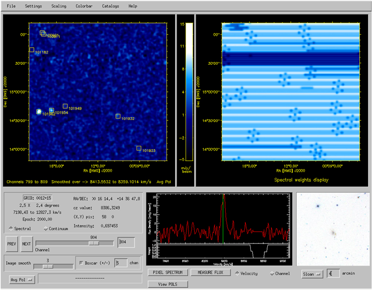
Figure 7. GridView application GUI created in IDL. The data-cube visualization procedure incorporates various IVOA web service tools for use during the data analysis process. The figure shows both optical image viewing and catalog overlay on the H i line zeroth-moment map over an adjustable range of channels (left). The display to the right of the moment map shows the corresponding weight map of the same region; horizontal stripes in the weights map reflect the interleaved drift-scan strategy and scalloped nature of coverage by beams of different gain. In that display, dark means low weight; there is a drift missing from this data set. The repeated pattern of seven darker spots represents the interruption of data-taking for the firing of the noise diode (every 600 s); the seven spots are the seven ALFA beams. The target under analysis here is AGC 101962, matching the brightest white spot on the left just below the center of the moment map. Its spectrum is shown near the center bottom; the spectral weight display, plotted underneath the flux density, indicates that the spectral range near the galaxy's H i emission is fine, but the spectral region around 8700 km s−1 is of low weight due to excision of RFI generated by the NUDET instrument on the GPS constellation of satellites and an internal modulation of the FAA radar. The bottom right window displays the SDSS r-band image of the field centered on the H i centroid. Users are able to manipulate the 3D spectral grid with the various GUI controls, export maps, view polarizations separately, and examine the spectrum corresponding to any grid pixel.
Download figure:
Standard image High-resolution imageAs mentioned in Section 2.4, H i line candidates are identified in the final grids by applying a matched filter algorithm in the Fourier domain (Saintonge 2007). The candidates are then examined and parameters measured individually using the tool GridView. An example of a GridView application is given in Figure 7. Importantly, GridView allows the manipulation (smoothing, comparing polarizations etc.) of channel maps, as well as the examination of the weight and continuum maps and the overlay and cross reference of complementary data sets, redshift catalogs, and imaging databases. This functionality is important for the final catalog data quality and critical for the identification of the probable OCs.
Identified sources are then run through the routine GalFlux, which measures fluxes and spectral parameters, allows cross-referencing with other databases, and produces the final data products for each detection. The user selects the region over which the spectrum will be measured. A "postage stamp" is extracted, isophotes are fit in the spatial domain, and the spectrum is displayed. Elliptical isophotes are automatically computed at levels of half and one-quarter of the peak power and 100, 200, 300, 500, and 1000 mJy beam−1; custom isophotes could also be fit. The interactive examination of the isophotes allows the user to refine the boundaries in both spatial and spectral dimensions and the baseline fit. The user then can make adjustments to the spatial and spectral boundaries and perform additional baseline fitting, smoothing, etc. to determine the best spectral and spatial definition of the H i line signal. Most often, the metric used to judge the best fit is the S/N; if the boundaries are too large, noise will drive the S/N down. In the majority of sources, such choices were not important, but this flexibility allows the user to make decisions about the best fit in the presence of low S/N, confusion, RFI contamination, polarization mismatch, or proximity to Galactic H i line emission and note evidence of extended sources or other peculiarity. Such examination can even result in source rejection; for example, if the feature is very narrow in velocity, and its spatial definition is inconsistent with the beam pattern, the source is highly likely to be spurious. The half-peak power isophote is typically larger than the ALFA beam FWHM and should contain all of the flux for sources of an extent comparable to or smaller than the beam. It should be noted, however, that in the vast majority of sources, the true H i extent is not known but is expected to be smaller than the beam. As noted previously, flux may be missing from very extended or asymmetric sources when this pipeline approach is used. A separate work will present fluxes for the known extended sources (G. L. Hoffman et al. 2018, in preparation).
Once the user is confident of the source definition, the flux and velocity measurement algorithm, as described in Section 2.5, is applied to produce a display of the postage stamp, isophotal fits, baselined spectrum, and associated weights over the isophote at 50% of the peak flux and measures of the integrated flux, velocities, velocity widths, and their error. In addition to statistical errors on the H i line flux density, velocity, and velocity width, systematic uncertainties on each value are estimated by flagging minimum and maximum estimates of the extent of the spectral feature and then using the ratio of those values to estimate uncertainties. In most cases, the systematic uncertainty is less than the statistical one and can be ignored. In cases of, e.g., low S/N, shallow profile outer slope, or RFI contamination, the statistical error can be clearly too small, and the uncertainty is set as the sum in quadrature of the two. Optical databases (SDSS, SkyView, and NED) can be accessed and displayed so that the user can assign the most probable OC. The user assigns the detection category and can enter comments about the source, extracted source, optical environment, etc. The final step in the analysis of a source is the production of a final output file containing all of the above information.
An additional GUI, depicted in Figure 8, enables the examination of a catalog of H i line sources and their corresponding "source" file. Individual sources can be selected from the catalog listing (top left); the isophotal fits (bottom left), spectrum and associated weights (bottom center), and corresponding optical field (bottom right) are displayed along with a summary of the derived and assigned parameters. A user can update parameters if additional information becomes available; the latter capability has been an important component over the years.

Figure 8. GalCat application GUI created in IDL. The catalog of ALFALFA sources is displayed as a list at top left. For each source selected from that list, a summary is presented in the interface, including the measured parameters (top center), the isophotal fits (bottom left), the extracted "postage stamp" spectrum and its normalized weight at each spectral point (bottom center), and the optical image (bottom right). The top right panel offers the possibility to modify parameters as necessary.
Download figure:
Standard image High-resolution image
Additional routines allow production of the catalogs, application of the adopted flow model (Masters 2005), and derivation of the H i masses. The full ALFALFA data reduction package, dubbed "Lovedata" (because we love our data), has been exported to over 50 sites.