


Abstract
Shock waves are believed to play an important role in plasma heating. The shock-like temporal jumps in radiation intensity and Doppler shift have been identified in the solar atmosphere. However, a quantitative diagnosis of the shocks in the solar atmosphere is still lacking, seriously hindering the understanding of shock dissipative heating of the solar atmosphere. Here, we propose a new method to realize the goal of the shock quantitative diagnosis, based on Rankine–Hugoniot equations and taking the advantages of simultaneous imaging and spectroscopic observations from, e.g., IRIS (Interface Region Imaging Spectrograph). Because of this method, the key parameters of shock candidates can be derived, such as the bulk velocity and temperature of the plasma in the upstream and downstream, the propagation speed and direction. The method is applied to the shock candidates observed by IRIS, and the overall characteristics of the shocks are revealed quantitatively for the first time. This method is also tested with the help of forward modeling, i.e., virtual observations of simulated shocks. The parameters obtained from the method are consistent with the parameters of the shock formed in the model and are independent of the viewing direction. Therefore, the method we proposed here is applicable to the quantitative and comprehensive diagnosis of the observed shocks in the solar atmosphere.
Export citation and abstract BibTeX RIS
1. Introduction
Sunspot oscillations are periodic intensity disturbances observed in the photosphere, chromosphere and transition region. This phenomenon was discovered by Beckers & Tallant (1969) in Ca ii H and K lines of the umbra. For historical reasons, the sunspot oscillations are broadly divided into three categories (Bogdan 2000): 5-minute oscillations, 3-minute oscillations, and running penumbral waves. The running penumbral waves are compressible oscillations observed in the penumbra (Giovanelli 1972; Zirin & Stein 1972). Recently, a clear linkage between running penumbral waves (5-min) and umbral oscillations (3-min) was reported. It is found that when running penumbral waves crosses the umbral boundary, part of the wavefront seems to get reflected back and propagates into the umbral center, where it expands radially (which means that a new umbral oscillation begins) and initiates the new running penumbral wave (Su et al. 2016; Priya et al. 2018). The 5-minute oscillations always appear in the photosphere of umbra (Bhatnagar et al. 1972), while the 3-minute oscillations can be observed in the photosphere, chromosphere, and transition region of umbra (Beckers & Schultz 1972; Bhatnagar & Tanaka 1972; Gurman et al. 1982). Both the 3-minute and 5-minute umbral oscillations are interpreted as compressive acoustic disturbances. The 3-minute oscillations in the chromosphere are regarded as the high-frequency tail of the oscillations in the photosphere (Bogdan & Judge 2006), and Brynildsen et al. (2000) suggested a close connection between the oscillations in the chromosphere and that in the transition region. When leaked into the corona, the compressive acoustic waves (i.e., quasi-parallel slow magnetosonic waves) can lead to the observed propagation of intensity disturbance (PID; Ofman et al. 1997; DeForest & Gurman 1998; Banerjee et al. 2000; Nakariakov et al. 2000; de Moortel 2009; Jiao et al. 2015). The dissipation of slow magnetosonic waves may be responsible for the asymmetry of the emission line profile due to the Landau resonance between the waves and the beam flow plasmas (Ruan et al. 2016) and may partly answer the debate on what the nature of the PID is (slow mode waves or intermittent upflows; Wang et al. 2009; De Pontieu & McIntosh 2010; Tian et al. 2011, 2012).
The acoustic waves are likely to be amplified and become nonlinear when they propagate upward from the underlying photosphere, as the atmospheric plasma density decreases rapidly (de la Cruz Rodríguez et al. 2013). For this reason, nonlinear sunspot oscillations, which have saw-tooth profiles, are frequently observed in the chromospheric and transition region's lines (Thomas et al. 1984; Bard & Carlsson 1997; Brynildsen et al. 1999, 2000; Rouppe van der Voort et al. 2003; Felipe et al. 2010; Tian et al. 2014). In these observations, sudden blueward shifts followed by slower transition to redward shifts can be found in the profiles of Doppler velocity and spectral line center. The sudden change of Doppler velocity or spectral line center are widely interpreted as the signal of shock waves (Bard & Carlsson 1997; Rouppe van der Voort et al. 2003; Felipe et al. 2010; Tian et al. 2014; Zhang et al. 2017), while Brynildsen et al. (1999) and Brynildsen et al. (2004) suggest that the oscillations are nonlinear waves without shocks. So whether the jump in spectral profiles is a shock or just a nonlinear compressional wave still remains an open question yet to be solved.
Shocks may play an important role in the dynamics of solar atmosphere. They have been suggested as an energy source for the heating of the solar atmosphere (Hollweg 1982) and are believed to drive most chromospheric jets in active regions (Hansteen et al. 2006). Shock waves can also serve as probes of the solar atmosphere, as the propagating characteristics of the waves contain valuable information about the structure of the atmosphere, which supports their propagation (Lites 1992). Therefore, it is meaningful to study the shocks in the solar atmosphere. In the studies of shocks, it is important to know their parameters (such as amplitudes and propagating speeds). For example, the information of shocks' amplitudes is necessary in evaluating the energy transported by the shocks. However, the overall characteristics of the shock are still a mystery, yet to be diagnosed and revealed observationally.
As motivated by the confronted challenges, we propose a new method to diagnose the parameters of observed shocks. The new method tries to make full use of all aspects of observational information and apply them to R–H equations (Section 2). By invoking this method, one can obtain the comprehensive features of the observed shocks: the propagating speed and direction of shocks, and the bulk velocities and temperatures of plasmas in the upstream and downstream. The new method is then applied to the shocks observed from IRIS and reveals the all-around characteristics of shocks by providing reasonable results (Section 3). The difference between the derived parameters and the real parameters as well as the dependence of the derived parameters on the viewing direction are further evaluated with the help of forward modeling (Section 4). The derived parameters from two different viewing directions are similar and comparable to the real parameters, suggesting that the new method is reliable and is independent of the viewing direction. A summary and discussion is given in Section 5.
2. Method
To estimate the parameters of shocks (e.g., the bulk velocities upstream and downstream, and the propagating speed of the shock surface) from the observation data is a difficult task, even though the resolution of the instruments has a significant improvement. The solar telescope with an extension of an imaging spectrograph between the telescope and the photon recording device (e.g., CCD) on board the IRIS spacecraft usually provides two types of data: (1) a 2D spatial image and (2) a "spectroscopic + spatial" image (see Figure 1). The propagation of the shock is usually studied with the time–space plot obtained from the time evolution of the intensity image, while the bulk velocity is usually estimated from the Doppler shift of the spectral profile of the emission line. However, in order to diagnose the shock comprehensively, one needs to figure out a way to combine and adequately utilize both the imaging and the spectroscopic information. For example, only the component of the propagation velocity perpendicular to the line-of-sight (LOS) direction can be known from the time–space plot, while the Doppler velocity is just the component of bulk velocity vector parallel to the LOS direction. The angle between the LOS direction and the shock propagating direction is crucial in deriving the shock parameters. Therefore, in our method to derive the shock parameters, we start with estimating the angle with the help of two plausible approximations.
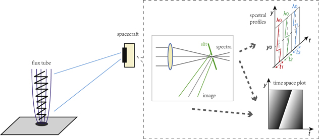
Figure 1. Sketch of both imaging and spectroscopic observation of the shock trains propagating in a flux tube by a telescope and a spectrograph on board a spacecraft. Like the optical path diagram design of IRIS (Interface Region Imaging Spectrograph), the slit splits the light into two branches, with one being reflected and reimaged to get to the 2D spatial image and the other passing through the grating system to get to the spectroscopic + spatial image.
Download figure:
Standard image High-resolution imageThe first approximation is the statistical equilibrium of the optically thin photon emission. The intensity of the observed emission line intensity is a function of squared plasma's density and temperature:

where I is the intensity of an emission line, and G(T) is the contribution function of the emission line. The contribution function is available in the CHIANTI Atomic Database (Del Zanna et al. 2015). This assumption is reasonable for the emission lines from the solar transition region, e.g., the Si iv line.
The second is to approximate the changes of states across shock with single-fluid Rankine–Hugoniot equations (R–H equations), which are usually used to describe the plasma conditions on two sides of the shock surface or discontinuity surface. In the rest frame of shock or discontinuity, the equations read (Boyd & Sanderson 2003, p. 187):


where ρ is the density of plasma,  is internal energy density, and u is the bulk velocity of plasma in the shock rest frame. The subscript numbers 1 and 2 stand for the upstream and downstream of the shock, respectively.
Suppose that the oscillation propagates in the solar atmosphere and is observed by a telescope from a certain viewing angle. The angle between the LOS direction and the wave propagating direction is θ, and the propagating speed is vp. We define that  is the component of the propagating speed vp parallel to the LOS direction,
  is the component perpendicular to the LOS direction (i.e., projected onto the plane of the sky). In the "laboratory" reference frame, Equations (2)–(4) can be converted to
where D, T, and M represent Doppler velocity, temperature, and Mach number, respectively. The ratio of density is given by
The Mach number upstream is given by

where local sound speed cs1 is a function of upstream temperature T1. The upstream velocity in the shock rest frame can also be given by

where  is upstream velocity in the "laboratory" reference frame.
The projection component of vp onto the plane of sky (POS), vβ can be obtained from the spacetime diagram of the wave propagation, Doppler velocities D1 and D2 are provided by the observed spectral data. Therefore, when Equations (8)–(10) are taken into account, Equations (5)–(7) have only three variables (T1, T2, and vα) to be solved: the upstream temperature T1, the downstream temperature T2, and the component of the propagating speed vα. With the information of vα and vβ, we can know the value of the angle θ:

The propagating speed of the shock and the full bulk velocities in the upstream and downstream regions can be known as well:


Therefore, with the shock diagnosis method as described above, one can estimate the comprehensive features of observed shock: the bulk velocities in the upstream and downstream, the temperatures in the upstream and downstream, the propagation speed and direction of shock.
Before applying this method to the observations of the solar lower atmosphere, one needs to be cautious and to address two questions. The first question is whether or not the chromospheric and transition region's emission lines are optically thin at the places of shock propagations. The chromosphere is a layer where radiative transfer is usually crucial and emission lines in this layer cannot be simply regarded as optically thin. Some lines such as Mg ii and C ii in regions like plage are optically thick, illustrating self-reversal and abnormal broadening spectral profiles. However, the optical depth of these lines in the umbra and penumbra regions of sunspots is smaller than that in plage regions, and the lines sometimes can be considered as optically thin, showing normal Gaussian and normal broadening profiles (see Figure 4 in Tian et al. 2014). In contrast, emission lines like Si iv from the layer of the transition region can always be regarded as optically thin. For example, both spectral profiles of Si iv line from the plage and umbra/penumbra regions appear normal Gaussian in Tian et al. (2014). Therefore, when employing this method, it is necessary to check whether or not the investigated spectral lines are optically thin in local regions.
The second question is whether or not the slope of shock-related brightness variations in the time–space plot ( ) of a transition region emission line can reflect the shock wavefront propagation through a spatial interval along the same flux tube. To address this question, two aspects needed to be considered. First, the thickness of the emission layer should be non-negligible to follow the shock wavefront propagation through a spatial interval along the same flux tube. Traditionally, in the old 1D hydrostatic models of solar atmosphere such as the VAL model (Vernazza et al. 1981), the whole transition region usually did not exceed 2 Mm in width. The altitude interval of a certain transition region emission line is much less than 1 Mm. Therefore, the shock wavefront would pass the emission line layer rapidly and the shock propagation along the same flux tube would be difficult to trace from the time–space plot. However, from the analysis of real observations, the transition region is found to extend over tens of Mm (e.g., Tu et al. 2005). The geometric thickness of the transition region emission lines C iv and Ne viii has been found to be larger than 2 Mm and 5 Mm (Tu et al. 2005), respectively, indicating that it is possible to trace the shock propagation through a spatial interval utilizing a certain transition region emission line in real solar observations. Furthermore, the thickness of the emission layer can be estimated from the shock propagation. When a shock front comes into the emission layer, the photons from both the upstream and downstream regions can contribute to the observed spectral profile leading to a double Gaussian profile, as long as the emitting sites are on the same line-of-sight path. Therefore, the thickness of the emission line layer (
 ) can be estimated from the time duration with a double Gaussian profile (tdg) and the wave propagation speed (vp). Second,
  can be contributed either by the propagation of the shock wavefront along the same flux tube or the sweeping of the wavefront across adjacent flux tubes. If
  is contributed by the sweeping of the wavefront across adjacent flux tubes, it will be significantly larger than the local acoustic speed, especially when the emission layer is oblique to the LOS direction. Otherwise,
  may be contributed by the propagation of the shock wavefront along the same flux tube. When employing this method, it is necessary to check if the thickness of the emission layer is non-negligible to follow the shock wavefront propagation through a spatial interval along the same flux tube and if the
  is less than the local acoustic speed.
For the observed shock-like waves (Tian et al. 2014), the Si iv line had a double Gaussian profile in a time duration of ∼ 30 s. If the propagating speed of the shock is reasonably assumed to be about 50 km s−1, the thickness of the Si iv emission layer would be ∼ 1.5 Mm, indicating that the thickness of the Si iv emission layer is non-negligible and possible to follow the shock wavefront propagation through a spatial interval along the same flux tube. Furthermore,  (∼25 km s−1) is quite less than the local acoustic speed (40–50 km s−1). Therefore, the slope of brightness variations in the time–space plot may reflect the shock wavefront propagation through a spatial interval along the same flux tube rather than sweeping across adjacent different flux tubes in the umbra. Then, the new method proposed here is applicable to the observations reported in Tian et al. (2014).
3. Application of the Method to Shock Observation
A detailed description of the application of the new method to the shock observations from IRIS (Tian et al. 2014) is given in this section. The time range of the IRIS data is from 16:39 to 17:59 on 2013 September 2. The spectral observation of Si iv 1393.76 Å and the slit-jaw image (SJI) 1400 Å are used. The slit is in sit-and-stare mode and centered at (99'', 58'') in the solar disk coordinates, and the spatial pixel size is 0 16. The cadence of 1393.76 Å and SJI 1400 Å are 3 s and 12 s respectively.
If the new method is applicable to the real solar observation, the derived results should satisfy the following two requirements: (1) the derived parameters of the observed shock should be reasonable and satisfy the basic shock properties; (2) the propagating direction derived from the two successively observed shocks at the same location should be consistent, because the structure of the solar atmosphere did not change a lot in several minutes. During the observation, lots of successive shock wave trains are caught by IRIS. The shock wave trains are roughly separated by ∼3 minutes.
The observations of two successive shock-like jumps and their propagation are illustrated in Figure 2). When the propagating direction in the plane of sky (POS) is not aligned with the spectral slit, the POS propagating speed vβ can only be obtained from the imaging observation, while when the propagating direction in the POS is aligned with the spectral slit,  can also be obtained from the spectral observation. For the observed shocks here, the propagating direction in the POS is aligned with the IRIS slit. Therefore,
  can be obtained from the spectral observation, such as the time–space plot of the intensity or the Doppler velocity. As shown in Figure 2(b),
  is obtained from the time–space plot of Doppler velocity of Si iv 1393.76 Å and the absolute slope of the two tilted black lines gives the values of
  for the two successive shock-like propagation. For the first shock (observed around
  ),
),  , a value well below local acoustic speed, indicating that the oblique patterns in the time–space plot represent the shock propagation along the same flux tube rather than sweeping across different flux tubes.

Figure 2. Panel (a): IRIS SJI 1400 image at 17:18:39 UT on 2013 September 2. The white vertical line labels the location of the IRIS slit and the two white horizontal lines indicate the spatial range shown in panel (b). The field of view of the SJI image has a size of 47'' × 47'' centered at (99'', 58''). Panel (b): the Doppler velocity of Si iv 1393.76 Å obtained from the single Gaussian fitting as a function of time (∼4.4 minutes since 17:18:39) and spatial locations marked by two white horizontal lines in panel (a). Panel (c): wavelength–time plot of Si iv 1393.76 Å at the location marked by the dashed black line in panel (b).
Download figure:
Standard image High-resolution imageFigure 3 shows how to get the upstream and downstream parameters of the shock. The total intensity in the upstream (0.48 minutes) and downstream (1.18 minutes) is 2872 (Iu) and 3640 (Id), respectively, and the Doppler velocity in the upstream and downstream is Du = 5.1 km s−1 and Dd = − 7.6 km s−1 respectively. With the aforementioned information, one can solve Equations (5)–(7) and derive the line-of-sight (LOS) propagating speed vα and the temperatures in the upstream (Tu) and downstream (Td). The acoustic speed is assumed to be  , where mp is the mass of a proton. The key parameters derived from the method are vα = 42 km s−1, Tu = 7.6 × 10⁴ K, and Td = 9.4 × 10⁴ K. Therefore, the propagating speed of the shock surface is
  , and the angle between the line of sight and the wave propagating directions is
  . The bulk velocity in the upstream and downstream are vu = −6.0 km s−1 and vd = 8.9 km s−1, respectively. All parameters of the observed shock are shown in Table 1. The plasma velocity in the upstream and downstream in the shock rest frame are
  and ud = vd − vp = −40 km s−1 respectively, while the local acoustic speed in the upstream and downstream are 44 km s−1 and 48 km s−1 respectively. Therefore, the plasma velocity in the upstream is supersonic (Mu ∼ 1.3) and that in the downstream is subsonic (Md ∼ 0.8), which is the necessary and sufficient conditions for the shock wave. This suggest that the derived results are reasonable.
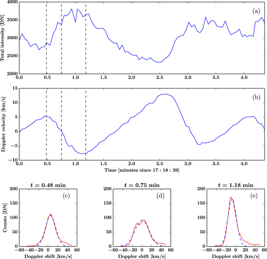
Figure 3. Temporal evolution of total intensity, Doppler velocity, and line profile of Si iv 1393.76 Å. Panel (a)–(b): the evolution of the total intensity and Doppler velocity of Si iv obtained from single Gaussian fitting. Panels (c)–(e): an example to show the evolution of the line profile of Si iv from upstream (panel (c)) to downstream (panel (e)). The profiles in red are the observed profile, while the dashed blue profiles are the single Gaussian fitting results.
Download figure:
Standard image High-resolution imageTable 1. The Parameters of the Two Shocks Obtained Directly from the Observation and Derived from the New Method
| Observation Data | Derived Results from the Method | |||||||||||||
|---|---|---|---|---|---|---|---|---|---|---|---|---|---|---|
| Iu | Id | Du | Dd | vβ | vα | Tu | Td | θ | vp | vu | vd | Mu | Md | |
| shock 1 | 2872 | 3640 | 5.1 | −7.6 | 25 | 42 | 7.6 | 9.4 | 31◦ | 49 | − 6.0 | 8.9 | 1.3 | 0.8 |
| shock 2 | 2321 | 3481 | 12.2 | −3.4 | 21 | 37 | 7.3 | 9.6 | 29◦ | 43 | −13.9 | 3.9 | 1.3 | 0.8 |
Note. I, D, v, T, and M are the intensity, Doppler velocity, bulk velocity, temperature, and Mach number. The subscripts u and d stand for the parameters in the upstream and downstream. vp is the propagating speed of the shock wave, while vβ and vα are the propagating speed in the POS and LOS respectively. θ is the angle between the LOS and the propagating direction of the shock wave. The units of intensity (I), velocity (D, v), and temperature (T) are (data number), [km s−1], and [104 K], respectively.
Download table as: ASCIITypeset image
For the second shock (observed around t = 3 minutes) shown in Figure 2. The total intensity in the upstream (t = 2.47 minutes) and downstream (t = 3.42 minutes) are Iu = 2321 and Id = 3481. The Doppler velocity in the upstream and downstream are Du = 12.2 km s−1 and Dd = − 3.4 km s−1. The propagating speed in the POS is vβ = 21 km s−1. The plasma velocity in the upstream and downstream in the shock rest frame are  and ud = vd – vp ≈ −39 km s−1 respectively. The plasma velocity of the second shock in the upstream is supersonic (Mu ∼ 1.3) and that in the downstream is subsonic (Md ∼ 0.8). The parameters of the second shock have been calculated and are listed in Table 1. Furthermore, the angle between the LOS and the propagating direction of the shock derived from the two successive observed shocks are similar, which further suggests that the results of this method are reliable.
4. Testing the Method by Numerical Simulation
The new method has also been benchmark tested with the help of numerical simulation. We simulate the evolution of shock waves with a numerical model. To mimic the remote sensing of the emitting shocks by an imaging spectragraph, we synthesize the spectra upstream and downstream of the shocks. The key parameters of the shocks are derived from the method and compared with the real shock parameters in the numerical modeling result. If the parameters derived from the method match well with the real parameters of the shock, it means that the new method is reliable to diagnose the shocks observed in the solar atmosphere.
The model used in the simulation is a kinetic model, which is described in Vocks & Marsch (2001) and Ruan et al. (2016). The governing equation of this model is the Boltzmann equation (Equation (4) in Ruan et al. 2016), in which the Coulomb collision term has been considered. In this model, we assume that the shock waves are propagating in a flux tube with an uniform cross-section. The diameter and height of the flux tube are set to be 1 Mm and 5 Mm, respectively. The bottom of the flux tube is located in the solar lower transition region. The initial conditions of the density, velocity, and temperature are displayed as dotted lines in Figure 4. The plasma, if approximated as fluid, is in an equilibrium state at t = 0. The gravitational acceleration (g) is set as g = − 274 m s−2, and the initial number density of proton decreases from Np = 1.0 × 10¹⁶ m−3 at h = 0 to Np = 3.5 × 10¹⁵ m−3 at h = 5 Mm. The initial bulk velocity of plasma is v = 0 and the initial temperature is T = 8 × 10⁴ K in the whole flux tube. The spatial extension of lower-transition-region temperature over more than 1 Mm is consistent with the observations (Tu et al. 2005). Heating and cooling terms, which are assumed to cancel one another out as a simplification, are not included in the governing equations of the simulation model.

Figure 4. Plasma condition along the flux tube. Panel (a): velocity distribution functions along the flux tube at t = 252 s. Panels (b)–(d): the number density, bulk velocity, and temperature profiles of protons along the flux tube at t = 252 s (solid curves) and t = 0 (dashed lines).
Download figure:
Standard image High-resolution imageIn order to produce the shock waves, slow mode waves are introduced at the lower boundary by imposing periodic fluctuations to the number density, bulk velocity, and temperature of the plasmas. The proton's number density, bulk velocity, and temperature at the lower boundary can be described as


where N0 = 1.0 × 10¹⁶ m−3, T0 = 8.0 × 10⁴ K, = 0.3 denotes the normalized amplitude of the perturbations, τ = 180 s is the period of the perturbations, and γ = 5/3 is the adiabatic index. The parameter  is the theoretical local sound speed, where p0 is background thermal pressure and ρ0 is background density at the bottom boundary.
Slow mode waves introduced at the lower boundary propagate upward and evolve into shock waves owing to the nonlinear effect. The location h = 3.0 Mm is chosen to conduct the evaluation of the new method proposed here. At t = 252 s, the slow mode waves have evolved into shock waves and arrive at h = 3 Mm (as shown in Figure 4(b)) with a propagating speed of vp = 45 km s−1. The velocity distribution function (VDF), number density, bulk velocity and temperature all show discontinuity patterns (shock surface). The width of the shock surface is about 150 km, which corresponds to the width of three grids in the simulation box (the width of one grid is 50 km). The width of the simulated shock surface is dependent on the grid width, and is always about two or three grids. The location h = 3 Mm lies in the upstream region at t = 222 s, while it lies in the downstream region at t = 282 s. In the upstream of the shock, the number density, bulk velocity, and temperature of protons are Np = 3.9 × 10¹⁵ m−3, vb = − 6.0 km s−1, and T = 5.8 × 10⁴ K. Their counterparts in the downstream of the shock are Np = 7.6 × 10¹⁵ m−3, vb = 14.5 km s−1, and T = 10.8 × 10⁴ K. Even though the upstream and downstream are taken at the same location but different times, the plasma property in the upstream and downstream of the shock still follows the mass conservation (Equation (2)) as  ×
× ![$[{v}_{b}(t\,=222\,{\rm{s}})-{v}_{p}]\approx \,{N}_{p}(t\,=\,282\,{\rm{s}})$](https://content.cld.iop.org/journals/0004-637X/860/2/99/revision1/apjaac0f8ieqn24.gif)
![$[{v}_{b}(t=282\,{\rm{s}})-{v}_{p}]$](https://content.cld.iop.org/journals/0004-637X/860/2/99/revision1/apjaac0f8ieqn25.gif) , suggesting that the sit-and-stare observation of shocks in the solar atmosphere is reasonable to derive the key parameters of the observed shock.
, suggesting that the sit-and-stare observation of shocks in the solar atmosphere is reasonable to derive the key parameters of the observed shock.
In the real solar observation, the angle between the LOS direction and the shock propagation direction is flexible. To ensure the universal applicability of the new method to the real solar observation, the results from the new method should be independent of the viewing direction, which defines the angle between the LOS direction and the shock propagation direction. Here, two viewing directions have been selected to assess this concern: the first viewing direction is set to deviate from the shock propagation direction by an angle of θ1 = 60° (path 1; marked by dashed line 1 in Figure 5); the second viewing direction is θ2 = 30° (path 2; marked by dashed line 1 in Figure 5). If the derived parameters of the shock from these two viewing directions are similar and consistent with the real parameters, the new method can be robustly applied to the real solar observation regardless of the viewing direction.
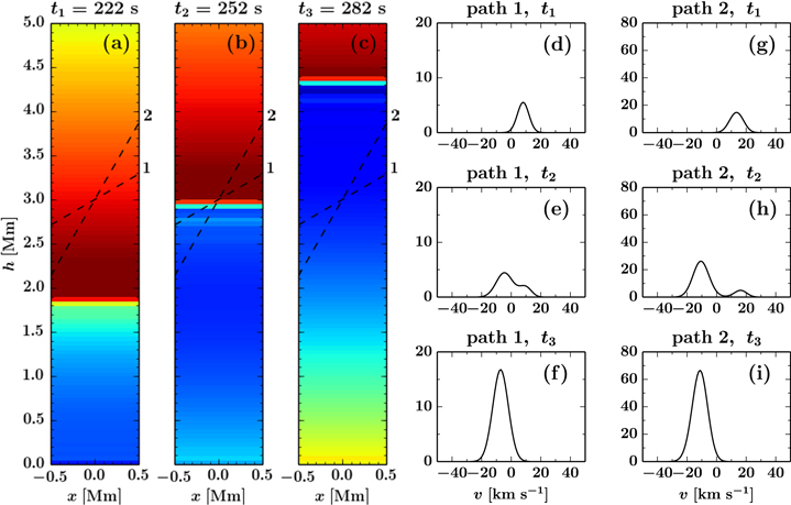
Figure 5. Panels (a)–(c): the simulated plasma velocity distribution in the 2D flux tube when the location h = 3 Mm lies in the upstream (panel (a); t1 = 222 s), at the shock surface (panel (b); t2 = 252 s), in the downstream (panel (c); t3 = 282 s). Paths 1 (dashed line 1) and 2 (dashed line 2) stand for two LOS paths to mimic the observation of the shock from two different viewing directions. Panel (d)–(f): the spectral profiles obtained from path 1 at t1, t2, t3. Panel (g)–(i): the spectral profiles obtained from path 2 at t1, t2, t3.
Download figure:
Standard image High-resolution imageAssuming the plasma is in the statistical equilibrium and neglecting the contribution of temperature's variation to the spectral intensity, the virtual emission from the local plasma can be described as  , where Ni is the number density of ions, T is the temperature, G(T) is the contribution function of the emission line and f(v) is the normalized VDF of ions. The virtual observed spectrum is the integration of Slocal along path 1 or 2. The nonthermal width of the spectrum is not considered here. Since the behaviors of the Si3+ ion are not simulated, the spectra of Si iv are obtained by assuming that NSi is proportional to Np, and the velocity of Si iv is equal to that of the proton (vb,Si = vb,p). The virtual spectra obtained from path 1 and path 2 are named spectra 1 and spectra 2 respectively. As shown in Figure 5, the two paths are located in the pure upstream and downstream at t1 = 222 s and t3 = 282 s, respectively; therefore, the spectra include only the information from the upstream or downstream and follow a single Gaussian distribution (Figure 5(d), (f), (g), and (i)); while the the two paths go from the upstream to the downstream at t2 = 252 s, and therefore the spectra are a mixture of the information from the upstream and downstream and show a double Gaussian shape (Figures 5(e) and (h)). The wavelength–time plot of the spectral intensity is very similar to the real observations (see Figure 2(c)). The line cores jump from maximum redshift to maximum blueshift, and then move slowly back to maximum redshift (Figures 6(a) and (c)). Owing to the different viewing direction, the maximum blueshifts (redshifts) of the spectra 1 and 2 are different, as well as the traces of the shock surface in the time–space plot.

Figure 6. Spectral profiles and time–space plots of spectrum 1 and spectrum 2. (a) Spectral profile of spectrum 1. (b) Time–space plot of spectrum 1. (c) Spectral profile of spectrum 2. (d) Time–space plot of spectrum 2.
Download figure:
Standard image High-resolution image
To benchmark test the new method, we first get some parameters of the shock that can likewise be obtained directly from the solar observation, such as the Doppler velocity and intensity in the upstream and downstream, and the propagating speed of the shock in the POS. Thereafter, the other key parameters of the shock are derived as that done for the observed shock in the solar atmosphere in Section 3. For spectra 1, the Doppler velocity in the upstream and downstream are Du1 = 8.04 km s−1 and Dd1 = −7.25 km s−1, while the intensity in the upstream and downstream are 54 and 221, respectively. For spectra 2, the Doppler velocity in the upstream and downstream are Du2 = 13.46 km s−1 and Dd2 = − 11.34 km s−1, while the intensity in the upstream and downstream are 173 and 874, respectively. The propagating speed in the POS of spectra 1 and 2 are vβ1 = 39 km s−1 and vβ2 = 21 km s−1, which are obtained from the slope of the dashed black lines in Figures 6(b) and (d). The propagating speed in the LOS vα, the upstream temperature Tu, and the downstream temperature Td are derived by solving Equations (5)–(7). Thereafter, the angle between the LOS and the wave propagating direction θ, the propagating speed of shock vp, the upstream velocity vu, and the downstream velocity vd are obtained from Equations (11)–(14). The results derived by applying the method to the virtual observations in two different viewing directions (paths 1 and 2) are similar and comparable to the modeling results (as shown in Table 2), suggesting that the new method is reliable and is independent of the viewing direction (the LOS direction).
Table 2. The Real Parameters of the Shock Wave, and the Parameters Derived for Two Different Viewing Directions 1 and 2, as Marked in Figure 5
| Iu | Id | Du | Dd | vβ | vα | vp | θ | vu | vd | Tu | Td | Mu | Md | ||
|---|---|---|---|---|---|---|---|---|---|---|---|---|---|---|---|
| Modeled | ⋯ | ⋯ | ⋯ | ⋯ | ⋯ | ⋯ | 45 | 60° | 30° | −16.0 | 14.5 | 5.8 | 10.8 | 1.5 | 0.6 |
| VirtualObs-1 | 54 | 221 | 8.04 | −7.25 | 39 | 28 | 48 | 54° | ⋯ | −14 | 12 | 6.1 | 9.4 | 1.5 | 0.7 |
| VirtualObs-2 | 173 | 874 | 13.46 | −11.34 | 21 | 43 | 48 | ⋯ | 26° | −15 | 13 | 6.0 | 9.3 | 1.5 | 0.7 |
Note. The derived parameters are labeled in red (viewing direction 1) and blue (viewing direction 2). I, D, v, T, and M are the intensity, Doppler velocity, bulk velocity, temperature, and Mach number. The subscripts u and d stand for the parameters in the upstream and downstream. vp is the propagating speed of the shock wave, while vβ and vα are the propagating speed in the POS and LOS respectively. θ is the angle between the LOS and the propagating direction of the shock wave. The units of intensity (I), velocity (D, v), and temperature (T) are (data number), [km s−1], and [104 K], respectively.
Download table as: ASCIITypeset image
5. Conclusion and Discussion
A shock wave, as a prevalent phenomenon in the solar atmosphere, is believed to play an important role in the evolution of solar atmosphere, such as the heating of the lower atmosphere. However, the quantitative and comprehensive diagnosis of the shock had not been investigated before this work. Here, based on the advantage of the simultaneous spectral and imaging observation from IRIS, we proposed a new method to fully reveal the quantitative characteristics of shocks. The method is summarized in the following four steps.
(Step-1) Before applying this method to the observation of lower solar atmosphere, it is necessary to check first if the spectral lines are optically thin in the local region of study and if the slope of the brightness variations in the time–space plot can reflect the shock wavefront propagation through a spatial interval along the same flux tube.
(Step-2) The propagating speed in the POS (vβ) is obtained from the time–space plot of the Doppler velocity or intensity. When the propagating direction in the POS is not aligned with the spectrograph slit, vβ can be obtained from the time–space plot of the intensity obtained from the imaging observation. When the propagating direction in the POS is aligned with the spectrograph slit, vβ can be obtained from the time–space plot of the intensity or Doppler velocity that is obtained from spectroscopic observation. The intensity and Doppler velocity in the upstream and downstream are estimated from the single Gaussian fitting to the spectral profile.
(Step-3) The propagating speed in the LOS (vα), the temperature in the upstream and downstream are derived with the help of Equations (5)–(7).
(Step-4) The bulk velocity in the upstream and downstream are calculated using Equations (13) and (14).
The new method has been applied to the shocks observed by IRIS and the derived parameters of the shocks are reasonable. The bulk velocity in the upstream and downstream are supersonic and subsonic respectively. Furthermore, the parameters derived from two successive shock waves are similar to each other. To evaluate the difference between the derived values and the real values of the shock parameters and the dependence of the method on the viewing direction, the method is also benchmark tested with the help of forward modeling. The emission spectral profiles of the plasmas are synthesized from two different viewing directions and used as virtual observational inputs to feed to the new method. The shock parameters derived from the virtual observations in the two different viewing directions are similar and comparable to the modeling results, suggesting that the new method is reliable and is independent of the viewing direction (the LOS direction). Therefore, we recommend employing this method as a standard approach to quantitatively and comprehensively investigate the shock itself and the consequent dynamical influences on the solar atmosphere.
J.-S.H., W.-Z.R., and L.-M.Y. are co-corresponding authors. The work at Peking University is supported by NSFC under contracts 41574168, 41474148, and 41421003. J.-S.H. is also supported by National Young Talent Program of China. The group from IGG/CAS is supported by NSFC under contracts 41704166, 41525016, 41474155, and 41661164034. L.-M.Y. is supported by National Postdoctoral Program for Innovative Talents (grant BX201600159) and Project funded by China Postdoctral Science Foundation (grant 2017M610978). We would like to thank Prof. Mingde Ding and Dr. Hui Tian for helpful discussions in the optical transparence and emission layer width of emission lines from lower transition region.