


Abstract
We present a set of four global Eulerian/semi-Lagrangian fluid solver (EULAG) hydrodynamical (HD) and magnetohydrodynamical (MHD) simulations of solar convection, two of which are restricted to the nominal convection zone, and the other two include an underlying stably stratified fluid layer. While all four simulations generate reasonably solar-like latitudinal differential rotation profiles where the equatorial region rotates faster than the polar regions, the rotational isocontours vary significantly among them. In particular, the purely HD simulation with a stable layer alone can break the Taylor–Proudman theorem and produce approximately radially oriented rotational isocontours at medium to high latitudes. We trace this effect to the buildup of a significant latitudinal temperature gradient in the stable fluid immediately beneath the convection zone, which imprints itself on the lower convection zone. It develops naturally in our simulations as a consequence of convective overshoot and rotational influence of rotation on convective energy fluxes. This favors the establishment of a thermal wind balance that allows evading the Taylor–Proudman constraint. A much smaller latitudinal temperature gradient develops in the companion MHD simulation that includes a stable fluid layer, reflecting the tapering of deep convective overshoot that occurs at medium to high latitudes, which is caused by the strong magnetic fields that accumulate across the base of the convection zone. The stable fluid layer also has a profound impact on the large-scale magnetic cycles developing in the two MHD simulations. Even though both simulations operate in the same convective parameter regime, the simulation that includes a stable layer eventually loses cyclicity and transits to a non-solar, steady quadrupolar state.
Export citation and abstract BibTeX RIS
1. Introduction
Differential rotation is a key energy source for the solar dynamo, and shapes the spatiotemporal evolution of the magnetic fields building up within the convection zone (e.g., Miesch & Toomre 2009; Charbonneau 2014, and references therein). The dynamical interaction between this dynamo-generated magnetic field and the underlying stably stratified fluid layer is highly complex, takes place across a rotational shear layer known as the tachocline (Spiegel & Zahn 1992), and is mediated in part by convective overshoot. Accumulation and further amplification of the magnetic field can take place within the tachocline itself, and may impact the characteristics of the magnetic cycles developing in the overlying convection zone. This can be due to direct magnetic backreaction on the differential rotation at its base, or to the development of large-scale magnetohydrodynamical instabilities (e.g., Spruit 2002; Miesch 2005; Lawson et al. 2015; Gilman 2017). Indirect magnetic influences on rotational dynamics are also possible via magnetically induced alterations of turbulent Reynolds stresses and convective energy fluxes, or through an alteration of the horizontal temperature contrast characterizing rotating stratified thermal convection (Kitchatinov & Ruediger 1995; Durney 1999), or even tachocline confinement (Forgács-Dajka & Petrovay 2001; Barnabé et al. 2017).
The basic angular momentum balance within the Sun's convection zone is usually taken to reflect a global (statistical) equilibrium between advection by the meridional flow and the rotationally induced Reynolds stresses (Tassoul 1978; Zahn 1992; Brummell et al. 1998; Brun et al. 2004, and references therein). The tachocline itself may also take part in the global angular momentum balance of the convection zone (see, e.g., Gilman et al. 1989), both in terms of providing vertical stresses mediated by the rotational shear, and in terms of latitudinal fluxes associated with large-scale flows, magnetic stresses and torques, and/or the development of hydrodynamical (HD) or magnetohydrodynamical (MHD) instabilities.
In view of the strong influence of rotation and convection and of the minute contribution of viscosity to the global force balance of the convection zone (Miesch 2005; Hanasoge et al. 2016), the Taylor–Proudman theorem is expected to constrain rotational isosurfaces to concentric cylinders centered on the rotation axis. This expectation is borne out by most global simulations of solar convection operating at relatively low, solar-like Rossby number (∼10−1), but stands in stark contrast to the nearly radial contours revealed by helioseismic rotational inversions for the bulk of the solar convection zone (Howe 2009). The thermal wind balance (Elliott et al. 2000; Brun & Toomre 2002; Miesch 2005; Miesch et al. 2006) that naturally develops in the presence of a latitudinal temperature gradient throughout the solar convection zone emerges as the most promising means to evade the Taylor–Proudman theorem. The presence of a latitudinal temperature (or entropy) gradient at the base of the convecting fluid layers can break the cylindrical alignment of isorotation countours expected from the Taylor–Proudman theorem (e.g., Rempel 2005; Balbus et al. 2009). Indeed, the mean-field calculations of Rempel (2005) as well as the global HD simulations of Brun & Toomre (2002) and Miesch et al. (2006) using the ASH code have amply confirmed this effect, although in these cases, this critical latitudinal gradient of temperature (or entropy) is artificially enforced through the boundary conditions.
Regardless of the causal chain, recent global MHD numerical simulations of solar convection certainly indicate that the presence or absence of a stable fluid layer leads to magnetic cycles showing distinctly different periods and spatiotemporal evolutions (see Guerrero et al. 2016a). Such global simulations, whether carried out in the MHD or purely HD regime, have also revealed that the solar internal differential rotation is quite sensitive to the parameter regime of convective dynamics. Relatively small changes in the Rossby number, for instance, can drive the latitudinal differential rotation from solar-like rotation, meaning a faster rotating equator than the poles, to a so-called anti-solar profile, with slower rotation in equatorial regions (see, e.g., Miesch & Toomre 2009; Charbonneau 2014; Gastine et al. 2014; Brun et al. 2017, and references therein). Such changes in internal differential rotation can in turn strongly impact the large-scale magnetic cycles developing in these MHD simulations, and quite possibly in the Sun and solar-type stars as well. Analysis of the output of some recent global MHD simulations of solar convection (e.g., Augustson et al. 2015; Strugarek et al. 2017) indicates that magnetically driven variations in internal differential rotation may be fundamental to the polarity reversals observed in these simulations.
In the present paper we use a set of four global simulations of solar convection obtained using the Eulerian/semi-Lagrangian fluid solver (EULAG) computational framework (Prusa et al. 2008; Smolarkiewicz & Charbonneau 2013) to investigate the means through which a latitudinal gradient can build up naturally at the base of the simulated convection zone, and under which conditions this can –or cannot–achieve the desired departure from the Taylor–Proudman theorem. In part because of the low dissipation levels they achieve at the larger spatial scales, EULAG simulations of solar MHD convection have been quite successful at producing stable decadal large-scale magnetic cycles (Ghizaru et al. 2010; Racine et al. 2011; Passos & Charbonneau 2014) showing a number of solar-like features, including patterns of torsional oscillations (Beaudoin et al. 2013), high-latitude meridional flows (Passos et al. 2015), secondary magnetic cycles (Beaudoin et al. 2016), and magnetically driven cyclic modulation of the convective energy flux (Cossette et al. 2013, 2017). Our most recent EULAG-MHD simulations (Strugarek et al. 2017), running at solar-like rotation rates and convective luminosities, have now achieved magnetic cycle periods very close to the period of the solar magnetic cycle (although they preferentially develop quadrupolar-like equatorial symmetry). While operating in a dissipative regime still far removed from solar interior conditions, these simulations nonetheless offer a valuable tool for investigating MHD effects that occur within the solar interior.
In this paper, we consider global simulations with and without a stable fluid layer below the convection zone, and with or without magnetism, which means that we consider four distinct cases. These four simulations are first described, and some of their salient properties are discussed, in Section 2. We then investigate the impact of the convective flux and the turbulence on the rotation profiles in all cases (Section 4). This is followed in Section 5 by an analysis of the thermal wind balance, fluctuating entropy, and pole-to-equator temperature differences. The impact of magnetism on convective flux and pole-to-equator temperature differences is considered in Section 6. A succinct conclusion follows in Section 7.
2. Four Global Simulations of Solar Convection
In order to understand the impact of both the stable layer and magnetism on the rotational properties, convective structures, and energy transport in a simulation of a solar-like convective envelope, we generate four distinct global convection simulations: two HD cases and two MHD cases, each either with or without an underlying stable layer. In what follows, these four cases are identified by the abbreviations HDcz, HDs, MHDcz, and MHDs, respectively, where "cz" indicates "convection zone only" and "s" stands for "includes a stable layer."
2.1. Numerical Formalism
The EULAG computational framework is used to generate all simulations we report in the following sections. The overall simulation setup closely follows the setup presented in Strugarek et al. (2016, 2017), the primary difference being the introduction of a convectively stable fluid layer that underlies the simulated convection zone.
The Lantz–Braginsky–Roberts equations (Lantz & Fan 1999; Braginsky & Roberts 1995), or equivalently, the Lipps–Hemler equations (Lipps & Hemler 1982, 1985), are solved for perturbed quantities with respect to an ambient state satisfying hydrostatic equilibrium. The Eulerian (flux form) integration scheme is used in solving these anelastic equations, which are projected onto a geospherical coordinate system (Prusa & Smolarkiewicz 2003; Smolarkiewicz & Charbonneau 2013). Advection is modeled using the multidimensional positive definite advection and transport algorithm (MPDATA), a class of nonoscillatory Lax–Wendroff schemes (Smolarkiewicz 2006). EULAG can operate as an implicit large-eddy simulation (ILES), which means that all dissipation is delegated to MPDATA, thus providing an implicit subgrid model (Domaradzki et al. 2003; Strugarek et al. 2016). An interesting property of the MPDATA dissipation is that it only "turns on" intermittently in space and time, whenever and wherever it is needed to maintain locally smooth (spurious-oscillation free) solutions, thus enforcing numerical stability (Smolarkiewicz & Charbonneau 2013). It is also adaptive, in the sense that implicit dissipation automatically vanishes if explicit dissipation is introduced in the model (Smolarkiewicz & Szmelter 2009). The time integration of linear forcing terms is carried out using a second-order Crank–Nicolson scheme.
Relevant equations in the convection zone for perturbed quantities with respect to the ambient state are written as


and a standard perfect gas equation of state, linearized around the background state. Here,  and
and  are the velocity and the magnetic fields, respectively, while Θ represents the potential temperature (related to the entropy σ via
  , with cp the specific heat at constant pressure). Operators D/Dt and ∇ have their usual meanings, with
  the material derivative. Gravity is defined as
  , with G and M being the gravitational constant and the solar mass, respectively, and μ is the magnetic permeability.
  is the angular velocity of the rotating frame in the
  direction, defined as the axis going from south to north pole. We set Ω0 = 3.08155 × 10⁻⁶ s−1, which corresponds to a solar-like rotation period of 23.6 days. The primes in the equations denote the deviation with respect to the ambient state (denoted with the subscript "a"), and overbars represent the background state. For the simulations considered here, the background and ambient states are identical except for the potential temperature; this differs from previously published EULAG global solar simulations (Ghizaru et al. 2010; Racine et al. 2011) in which ambient and reference states were characterized by slightly different density stratifications. The quantity π' encompasses both fluid and magnetic pressures and is a global pressure perturbation with respect to the ambient state.
  is the ambient/background state of mass density. Explicit viscous and Ohmic dissipative terms are omitted. All ambient/background states
  ,
,  ,
,  , Θa, and
  are defined exactly as in Strugarek et al. (2016) for the convection zone. Convection is forced through the advection of the unstable ambient entropy profile (characterized by the ambient potential temperature Θa) and the Newtonian cooling term, operating on a timescale τ = 5.184 × 10⁷ s, largely exceeding the convective overturning time at the base of the convecting layers.
2.2. Domain, Resolution, and Boundary Conditions
In order to allow long temporal integrations, the spatial resolution in the cases with a convection zone only is set at nr × nλ × nϕ = 51 × 64 × 128. When an underlying stable fluid layer is included, 20 additional grid points in radius are added, so as to maintain the same vertical grid spacing in all four cases. The radial extent of the domain for cases without a stable layer and those with such a layer encompasses [Rb/R, Ro/R] = [0.7,1] and [Rb/R, Ro/R] = [0.58,1], respectively, where R is the actual radius of the Sun (even though the simulations do not capture the photospheric convective dynamics in any way), and the "b" and "o" subscripts indicate the bottom and top of the domain, respectively. The density stratification in the convectively unstable fluid layers spans Nρ = ln(ρi/ρo) = 3.22 scale heights, with ρi and ρo being the background density at the base of the convection zone (at the interface) and at the top of the domain, respectively. The entropy jump between the base of the convection zone and the top of the domain is set at Δσ = 1 J kg−1 K−1, and the density at the bottom of the convection zone in all cases is set at  .
.
Boundary conditions in all cases are the same: stress-free, impenetrable boundaries on the flows at the top and bottom of the domain, perfect conductor at the bottom, and radial magnetic field at the top for the MHDcz and MHDs simulations:


2.3. Stable Layer Implementation
In simulations including a convectively stable fluid layer, the same Equations (1)–(5) are solved concurrently, but with the Newtonian cooling term in Equation (2) turned off in that layer. The ambient and background states are smoothly extrapolated from the convection zone profiles, and a strong radial gradient in the ambient potential temperature is enforced so as to achieve a strongly subadiabatic stratification, as expected in the outer solar radiative zone. Convective overshoot is thus restricted to a very thin layer immediately beneath the nominal convection zone, again in qualitative agreement with helioseismic inversions of the solar internal structure. Figure 1 depicts background density and radial ambient potential temperature gradient profiles in simulations with and without a stable layer, shown in black and red, respectively. A closeup of the gradient is shown in the upper right corner of the plot to reveal its structure. Profiles in the convection zone are identical to what is used in Strugarek et al. (2016), with new stable layer profiles added as dotted lines. The choice of the radial ambient potential temperature gradient is arbitrary, as a boundary condition close to a (thermal) perfect wall at the interface was desired. In simulations HDs and MHDs, radial velocity absorbers are added at the very bottom of the domain to ensure the damping of gravity waves (e.g., Brun et al. 2011), which cannot be properly resolved by our relatively coarse spatial mesh.

Figure 1. Radial profiles of the background density (black) and the radial ambient potential temperature gradient (red). Solid and dotted lines correspond to profiles defined in the convection zone and the stable layer, respectively, with the vertical dashed line defining the interface. The inset replots the radial ambient temperature gradient on a different scale.
Download figure:
Standard image High-resolution image3. General Results
3.1. Differential Rotation
Considering that all physical input parameters are the same in all four cases considered, the rotational dynamics can only be altered by the presence of a magnetic field or angular momentum fluxes in or out of the convectively stable fluid layer. It is interesting to first compare differential rotation profiles. These are displayed in Figure 2 for each case in the same color scale in meridional slices. Working in the statistically stationary states of the simulations, rotational frequencies are averaged in longitude over a sufficiently large temporal extent to filter out signals associated with turbulence and magnetic field cycles, when present. In the two simulations that include a stable layer, a thin tachocline-like shear layer rapidly establishes itself immediately beneath the convective layers. Its sustained thinness is testimony to the very low dissipation characterizing the large spatial scales in these EULAG simulations (Strugarek et al. 2016). More generally, penetration of flows into the stable layer is minimal, restricted to a few percent of the solar radius. The differential rotation contrast in latitude, characterized by ΔΩ/Ω0 = (ΩN − ΩE)/Ω0, where ΩN is the mean value of rotation over the three northernmost grid points and ΩE is the same quantity averaged on three grid points at the equator, is listed for the four models in the first column of Table 1. The two HD cases display a stronger pole-to-equator contrast in rotation frequency, amounting to ∼32% in HDcz and ∼38% in HDs (poles are saturated to better show trends at mid-latitudes). The contrast in HDs is greater than in HDcz, even though the equatorial frequency is lower in that case, which means that the poles are rotating slower than in HDcz. Pole-to-equator contrasts are much lower in the MHD cases, where the values for MHDcz and MHDs are ∼17% and ∼15%, respectively. This backreaction of the magnetic field on the rotation frequency is well documented in these types of simulations (Gilman & Miller 1981; Gilman 1983; Brun et al. 2004; Beaudoin et al. 2013).

Figure 2. Polar representations of rotation frequencies in all simulations, showing the differential rotation profiles. Flows have been averaged both in longitude and in time (more than 300 rotation periods), the latter being on a time period sufficiently long to have a good statistical sample (in MHD cases, the time interval used is identified in Figure 3). Dashed circular arcs in panels (C) and (D) indicate the base location of the nominal convection zone (superadiabatic ambient stratification).
Download figure:
Standard image High-resolution imageTable 1. Global Properties of the Simulations
| ΔΩ/Ω0 |
 (K) (K) |
 (K) (K) |
EB/Eu | |
|---|---|---|---|---|
| HDcz | 32% | 12.07 | ⋯ | ⋯ |
| HDs | 38% | 9.63 | 21.31 | ⋯ |
| MHDcz | 17% | 14.46 | ⋯ | 0.13 |
| MHDs(II) | 41% | 9.73 | 22.52 | 0.004 |
| MHDs(III) | 15% | 15.81 | 6.94 | 0.23 |
| MHDs(IV) | 10% | 16.44 | −0.75 | 0.85 |
Download table as: ASCIITypeset image
Looking at the four panels in Figure 2, one can identify the HDs case as having the most solar-like rotational isocontours in the convection zone: sharp pole-to-equator contrast (equator rotating faster than the poles), with the stable layer rotating at a frequency intermediate between that of pole and equator; approximately radial isocontours at medium to high latitudes; and the presence of a tachocline-like shear layer. Notwithstanding the lower pole-to-equator contrast in rotation rate in the two MHD simulations compared to their HD counterparts, on the basis of Figure 2 one already notes that the addition of a stable layer has as much impact on the overall shape of the rotational isocontours as the inclusion of a magnetic field.
3.2. Large-scale Magnetic Field
The two MHD simulations operate in a physical regime where a large-scale magnetic field is produced through dynamo action. Figure 3 illustrates the longitudinally averaged toroidal magnetic field building up in these simulations, in the form of latitude–time and radius–time diagrams. The MHDcz case is plotted on the same temporal extent as MHDs, which explains the apparent "missing data" at t > 495 years in panels (A) and (B). The vertically dashed lines delimit the averaging time intervals used in the analyses we present below (and in Figures 2(B) and (D)).

Figure 3. Latitude–time (panels (A) and (C)) and radius–time (panels (B) and (D)) diagrams of the longitudinally averaged toroidal magnetic field in the two MHD simulations. In both cases the diagrams are extracted at the same depth (r/R = 0.72) and latitude (λ = 58 5). The dashed horizontal black line in panels (B) and (D) indicates the location of the base of the convection zone. The vertical dashed black lines delimit the temporal intervals across which temporal averages have been taken for the purposes of the foregoing analyses. The vertical dashed white lines delineate the four dynamo "phases" in simulation MHDs.
Download figure:
Standard image High-resolution imageThe MHDcz case (panels A and B) is identical to Model 1 (Figure S1) presented in the supplementary materials of Strugarek et al. (2017). Panel (A) is a time–latitude slice extracted near the bottom of the convection zone, 0.02 R away from the bottom domain boundary at r/R = 0.7. Panel (B) is a radius–time cut taken at a latitude where the mean magnetic field reaches peak strength. Quite a few solar-like features in the mean toroidal magnetic field are plotted in these panels, such as (1) a strong axisymmetric component; (2) cyclic polarity reversals of the large-scale magnetic field unfolding over a ≃25-year period, which is quite close to the solar cycle magnetic period; (3) equatorward propagation of the large-scale magnetic field; and (4) accumulation of the toroidal magnetic field near the interface, the location where magnetic flux ropes giving rise to sunspots are traditionally believed to be formed and stored (see Fan 2009, and references therein). However, and in contrast to the Sun, the MHDcz simulation develops and maintains a symmetric equatorial parity, and the magnetic flux peaks at mid-latitudes instead of at the lower latitudes that are indicated by the sunspot butterfly diagram. Nonetheless, reasonably solar-like large-scale convective dynamo action is taking place here entirely within the convection zone without the need of a tachocline or, more generally, of an underlying stable fluid layer.
Panels (C) and (D) of Figure 3 display the zonally averaged toroidal magnetic component building up in the MHDs simulation in the same format as in panels (A) and (B) for MHDcz. The spatiotemporal evolution of the large-scale magnetic field is markedly different in these two MHD simulations. This case is interesting in several ways, such as the presence of multiple dynamo "phases" and transitions and the marked accumulation of toroidal magnetic field below the interface. Four fairly distinct phases can be identified in this simulation. The first, ending at about 70 years, is almost purely HD, in the sense that very little magnetic field builds up over this time period, even though convection and differential rotation rapidly reach a statistically stationary state. The second phase, ranging from ∼70 to ∼240 years, witnesses the appearance of a highly turbulent magnetic field, with a weak (<0.1 T) axisymmetric component peaking near the top and bottom of the convection zone, and it undergoes irregular polarity reversals on a timescale of a few years. This "fast cycle" appears similar to the secondary dynamo mode observed in the EULAG "millenium simulation" (see Passos & Charbonneau 2014), that was analyzed in detail in Beaudoin et al. (2016). The third phase, ranging from ∼240 to ∼400 years, produces arguably the most solar-like dynamo signature. One observes an accumulation of axisymmetric magnetic field near the interface and in the stable layer, this field being largely antisymmetric about the equator, in accordance with solar inferences. This third phase resembles the MHDcz simulation most closely in terms of overall magnetic field strength, accumulation of magnetic field at medium to high latitudes and near the interface, and a similar radial structure in the convection zone. Consequently, this phase is used for further comparison with MHDcz. Note also that while the latter builds up a large-scale magnetic field that is dominantly axisymmetric, in phases two and three of MHDs, the large-scale magnetic field is characterized by a non-axisymmetric component containing at least as much magnetic energy as the axisymmetric component. This non-axisymmetric component is filtered out in the zonal averages displayed in panels (C) and (D) of Figure 3. The fourth and final phase, which extends from ∼400 years until the end of the simulation, is characterized by a dominantly axisymmetric, and equatorially symmetric, steady quadrupolar-like large-scale magnetic configuration, with a very strong magnetic field (∼1 T) that accumulates deep in the stable fluid layers.
Table 1 lists some salient global properties of the four simulations: (1) normalized pole-to-equator rotational contrast, (2) pole-to-equator temperature differences near the surface ( ) and (3) below the interface (
 ), and finally, (4) the ratio of volume-integrated magnetic energy to kinetic energy. Roman numbers associated with the MHDs simulation identify the "phase" in which these quantities are calculated.
3.3. Angular Momentum Fluxes
Following Brun et al. (2004) and Beaudoin et al. (2013),3 we now investigate quantitatively the differential rotation dynamics in our four simulations by computing radial and latitudinal angular momentum fluxes. These quantities are defined as
where the operator  denotes a longitudinal average,
  defines the non-axisymmetric components, and λ is the latitudinal coordinate (as opposed to the conventional polar angle). The terms
  ,
,  ,
,  , and
, and  , where i = r, λ, are the Reynolds stresses, the Coriolis force acting on the meridional circulation, and the torques due to the non-axisymmetric and axisymmetric components of the magnetic fields, respectively.
The next step is to integrate Equation (8) over constant-radius shells and Equation (9) over conical surfaces of constant latitudinal angle to obtain global angular momentum transport rates:


Figure 4 plots the result of this analysis for our four simulations, with each color-coded curve corresponding to the contribution of each of the four (MHD, solid lines) or two (HD, dashed lines) terms on the right-hand side (RHS) of Equations (8)–(9). The contributions of the various terms are remarkably similar in all simulations, in particular in the case of radial transport (left panels). As in Guerrero et al. (2016b), Reynolds stresses pump angular momentum inward. Here, accumulation takes place in the outer half of the convection zone, excluding subsurface layers (thus driving equatorial acceleration, see Figure 2.) Note in particular that the presence of magnetism (solid versus dashed curves) only has a minor impact on the radial angular momentum transport, and that the inclusion of the stable layer (top versus bottom panel) only alters the amplitude of the various terms, without changing their overall shape across the convection zone. It is also worth noting that with or without stable layers, the presence of magnetic fields affects radial transport primarily through an alteration of the Reynolds stresses and meridional flow contributions (cf. the solid and dashed blue/green curves within each panel on the left), rather than directly via magnetic torques, which remain very low in amplitude compared to the two HD contributions (on this point, see also Beaudoin et al. 2013), except at the base of the convection zone.

Figure 4. Radial (left column) and latitudinal (right column) angular momentum transport rates, both averaged in time and in latitude for the radial fluxes and in radius for the latitudinal fluxes. The vertical dashed lines in the diagrams in the left column indicate the base of the convection zone. In all panels the solid lines refer to MHD simulations, while dashed lines correspond to HD simulations. Each contribution is color-coded as follow: blue for the Reynolds stresses, green for the Coriolis force acting on the meridional circulation, orange for the non-axisymmetric components of the magnetic field, and red for the axisymmetric components of the magnetic field.
Download figure:
Standard image High-resolution imageIn the case of latitudinal transport (right panels), differences are more noticeable. Magnetic terms now contribute to the latitudinal transport at a level comparable to HD terms. The total magnetic contributions to latitudinal transport in MHDcz and MHDs (sum of red and orange curves) are in fact almost identical, the swap between the orange and red curves is an artifact of the analysis, as it simply reflects the dominance of the axisymmetric component in MHDcz, while in MHDs the non-axisymmetric fields dominate. The most striking difference is found with the meridional flow contribution, which shows an entirely different pattern at medium to low latitudes when a stable layer is included (cf. the green curves in the top right and top left panels). The inclusion of magnetic fields has comparatively less impact, altering the amplitudes, but not the overall shape of the latitudinal transport profiles (cf. the solid and dashed green curve in each panel). These magnetic contributions counterbalance the effect of the HD terms, especially the Reynolds stresses, which situation is similar to other simulations (Brun et al. 2004; Guerrero et al. 2016b).
Since the latitudinal transport rates result from integrating Equation (9) over all depths, the possibility remains that the strong impact of the stable layer on latitudinal angular momentum transport reflects processes that occur within the stable layer (Guerrero et al. 2016a), which are de facto absent in HDcz and MHDcz. However, repeating the calculation of Iλ by restricting the radial integral to the convection zone alone yields curves that are almost indistinguishable from those plotted in the two right panels of Figure 4. The presence of the stable layer indeed strongly influences latitudinal angular momentum transport throughout the convection zone. We now turn to this task.
4. Mean Convective Flux and Turbulence
The convective energy flux is defined as

where  indicates a horizontal average over all latitudes and longitudes, at fixed radius. This yields the mean convective energy flux as a function of depth. Panel (A) of Figure 5 shows these radial profiles of mean convective fluxes, further averaged over the same temporal intervals as were used in previous analyses. All four simulations show very similar profiles throughout most of the convection zone, MHD cases transporting roughly ∼20%–30% more energy in the upper convection zone than their HD counterparts. The presence of a stable layer does not impact the convective energy flux in most of the convection zone, except close to its nominal base in the HDs simulation. The convective flux is slightly negative just below the interface in the two simulations with a stable layer (not visible on the scale of this diagram), the more so the higher the latitude. Panels (B) to (E) offer a spatially resolved representation of convective fluxes, which allows distinguishing latitudinal dependencies. As anticipated from panel (A), no major differences are observed between the simulations, but some differences remain noteworthy, in particular the enhanced convective flux at high latitude in the HDs simulation, which peaks at the base of the convection zone. This enhancement is primarily responsible for the elevated mean flux at r/R = 0.7 for HDs in panel (A).

Figure 5. Convective energy fluxes in the four simulations. Panel (A) plots convective fluxes averaged horizontally and temporally for each case as a function of depth, with the vertical dashed line indicating the location of the interface between the convection zone and the stable layer. Different colors identify the cases, as indicated. Panels (B)–(E) depict longitudinally and temporally averaged convective fluxes for each case. Dashed circular arcs in panels (D) and (E) indicate the base convection zone. All temporal averages have been taken to have a good statistical sample (and to diminish the impact of the cycling large-scale magnetic field in MHD cases). The color scale is stretched to better show the low-amplitude variations.
Download figure:
Standard image High-resolution imageA more subtle difference arises when we compare the HD cases to their MHD counterparts, namely a small enhancement of the convective flux at medium to high latitudes in the latter that persists throughout the bulk of the convection zone. These regions are located radially above the latitude range where the magnetic field amplitude is maximal (see Figure 3). The presence of strong magnetic fields deep in the convection zone leads to a slight increase of the convective energy flux, feeding more energy overall to the outer layers. This enhancement is ultimately caused by the Lorentz force, and its dynamical underpinning is investigated in detail by Cossette et al. (2017) in the EULAG millenium simulation. Such effects notwithstanding, it is unlikely that they by themselves might lead to the observed large differences in internal differential rotation profiles (viz. Figure 2), as Figure 5 clearly shows that all four simulations operate very nearly in the same convective luminosity regime.
A different and useful look at the kinematics of convective turbulence is obtained from the probability density function (PDF) of vertical velocities at constant depth. Figure 6 shows such PDFs constructed from numerical data that were extracted in the main body of the convection zone at r/R = 0.8 (left), and just above its base, at r/R = 0.72 (right). The upflow/downflow asymmetry of these distributions arises from the requirement of mass conservation, and is characteristic of thermal convection in a density-stratified environment (see, e.g., Castaing et al. 1990; Cattaneo et al. 1991; Brummell et al. 1996; Brun et al. 2004). The presence of non-Gaussian "fat tails" is indicative of spatiotemporal intermittency in strongly turbulent flows. An obvious difference is the suppression of these extended tails in simulations without a stable layer, presumably reflecting the effect of the (impenetrable) lower boundary conditions that suppress radial flows near the bottom boundary. Phrased differently, including the stable layer allows convective overshoot and thus higher radial velocities near the bottom boundary, with possible enhancement of the convective energy fluxes.
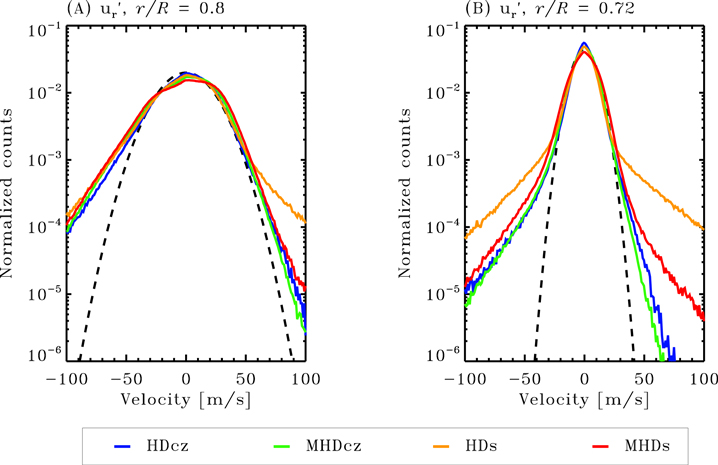
Figure 6. PDFs of the radial flow  at all grid points at a fixed depth. Panel (A) shows the distribution of values at r/R = 0.8 and (B) at r/R = 0.72 for all four cases. Results are given for all four simulations, as color-coded. Note the upflow/downflow asymmetries, and the extended tails in the r/R = 0.72 PDFs for the HDs and MHDs simulations. The dashed parabolas are Gaussian profiles matching the peak of the distribution; they are provided to guide the eye.
Download figure:
Standard image High-resolution imageThis effect is reduced in the MHDs simulation because the strong magnetic fields that are present at high latitudes provide an additional force that opposes upflows and downflows (on this point, see in particular Cossette et al. 2017). This effect is hardly visible in the MHDcz simulations because the radial flow is already much lower near the base of the domain, where the magnetic fields accumulate and reach their peak strength (see Figure 3(B)).
This suppression of convective overshoot is readily apparent in Figure 7, which displays Mollweide projections of the vertical fluid velocity at the interface between the convection zone and the underlying stably stratified fluid layer. The latitudinally elongated flow structures stacked along the equator are the residual imprints of the so-called banana cells that are commonly found in convection rotating at low Rossby numbers in thick spherical shells (Brun et al. 2004; Miesch & Toomre 2009; Ghizaru et al. 2010; Käpylä et al. 2010). Otherwise, upflows and downflows are distributed at all latitudes and are more vigorous at high latitudes in the HDs simulation. No such pattern is seen in the MHDs simulation on the left, which is again indicative of the suppression of radial flow by the strong magnetic fields that build up at medium to high latitudes deep in this simulation. Indeed, the strong upflows and downflows that are visible at high latitudes in Figure 7(A) are responsible for the enhanced convective energy flux that is present at high latitudes Figure 5(D).

Figure 7. Mollweide snapshot of  at r/R = 0.7 in the two simulations with a stable layer. The time in both simulations is chosen so that they are in a statistically stable state regarding turbulence, and for the MHD case, at a maximum of the magnetic cycle within the temporal interval identified in Figure 3. Overshoot in panel (B) is strongly suppressed, especially at high latitudes.
Download figure:
Standard image High-resolution imageThis latitudinal variation of the convective energy flux, mediated by convective overshoot across the base of the convection zone, turns out to play a major role in setting the shape of the rotational isocontours throughout the bulk of the convection zone. We now examine this effect from the point of view of thermal wind balance.
5. Thermal Wind Balance
Returning to the momentum Equation (1), we consider a situation in which mean flows are in a statistically stationary state, and (implicit) viscous diffusion, Reynolds stresses, and Lorentz forces can be neglected. Upon zonal averaging, the horizontal and vertical components of (1) become statements of joint geostrophic and hydrostatic balance, respectively,

Taking the curl of this expression then yields for the longitudinal component
where λ is again the latitudinal coordinate. Equation (14) expresses the Taylor–Proudman constraint: with a perfectly adiabatic horizontal profile (∂Θ'/∂λ = 0), the zonal component must be independent of z, implying isorotation surfaces taking the form of concentric cylinders centered on the rotation axis (Pedlosky 1992; Miesch 2005). A non-zero latitudinal gradient in potential temperature (or, equivalently, entropy) becomes the only means of departing from cylindrical rotation in the physical regime under which Equation (14) is obtained.
A rotation profile satisfying Equation (14) is said to be in thermal wind balance. Following Brun & Toomre (2002), Figure 8 depicts how well thermal wind balance is achieved in our four simulations; the left-hand side (LHS) and RHS of Equation (14) are displayed in the meridional plane, along with its residual, which is defined as the LHS minus the RHS. In all cases, the residual is multiplied by a factor of 10 to better display its features. Away from the upper boundary, a satisfactory thermal wind balance is attained in all cases. Significant residuals are apparent deeper in the convection zone in polar regions, in particular for the HDs simulation, and to a lesser extent at the interface between the convection zone and the stable layer in both HDs and MHDs. These departures are likely associated with the action of Reynolds stresses in these regions of strong rotational shear (on this point, see also Brun et al. 2010).

Figure 8. Depiction of the thermal wind balance equation in each simulation, from top to bottom. From left to right, LHS of Equation (14), RHS of that same equation, and the residual (LHS–RHS), its amplitude multiplied by 10. Dashed circular arcs in the bottom two rows indicate the location of the convection zone/stable layer interface.
Download figure:
Standard image High-resolution imageOther ways to ascertain thermal wind balance are to either compute the residual entropy σ', defined as

or to calculate the pole-to-equator physical temperature differences. Residual entropy is a quantity of interest because convective upflows and downflows, dominating convective energy transport, are expected to align along constant σ' surfaces. Moreover, as argued by Balbus et al. (2009), they should also coincide with isorotational contours, thus implying a strong correlation between these two quantities.
A comparison between color maps of residual entropy, with differential rotation isocontours superimposed, is presented in the top four panels of Figure 9, again in meridional plane representations. Although less impressive than the case presented in Balbus et al. (2009; see their Figure 2), away from the boundaries and poles, an overall similarity between the two sets of contours is apparent, especially in equatorial regions. Note in particular that in the HDs simulation, both sets of isocontours are markedly radial at medium to high latitudes in the bottom half of the convection zone. The strong latitudinal gradient of residual entropy in the upper reaches of the stable fluid layer is also remarkable; it lies immediately beneath the base of the convection zone, a feature that has no counterpart in the two simulations without stable layers.

Figure 9. Meridional slices of fluctuating entropy (color scale) with superimposed isocontours of the angular velocity (panels A–D) and the pole-to-equator temperature difference for each simulation (panel E). Rotation isocontour saturations are defined as 420 nHz < Ω/2π < 560 nHz for all top four panels. The dashed lines in panels (A)–(D) and the vertical dashed line in panel (E) denote the location of the interface between the stable layer and the convection zone. Pole-to-equator temperature differences are taken with respect to the north pole, but essentially indistinguishable results are obtained using the south pole instead.
Download figure:
Standard image High-resolution imageThe bottom panel of Figure 9 depicts the depth variation of the pole-to-equator difference in physical temperature perturbations (T'), related to potential temperature perturbation Θ' via

North and south pole-to-equator temperature differences are indistinguishable on the scale of these plots. These temperature differences presented in panel (E) of Figure 9 are obtained when subtracting the temperature averaged over the three northernmost grid points from the same quantity taken at the equator. Nominal values taken just below the surface and the interface are listed in Table 1.
In all cases there is a significant pole-to-equator temperature difference in subsurface layers, resulting from rotational influence on convective energy transport across the convection zone, which is a well-documented feature of thermally driven convection in rotating spherical shells (see, e.g., Miesch 2005, and references therein). In the parameter regime of our simulations, this influence is most visible in the structuring of convective flows, organized as latitudinally elongated banana cells at low latitudes and smaller, more vigorous convection cells at high latitudes, achieving a more efficient upward heat transport. This latitudinal pattern is a direct reflection of the impact of the Coriolis force on convective flows. Interestingly, the subsurface latitudinal temperature contrast is significantly higher in the MHD simulations than in their HD counterpart. This likely reflects the impact of the Lorentz force on the dynamics of upflows and downflows, as investigated in detail in Cossette et al. (2017) in a distinct but closely related EULAG simulation.
Of greater interest in the context of rotational dynamics is the significant pole-to-equator temperature contrast that develops immediately beneath the base of the convecting fluid layers in the two simulations that include a stable fluid layer. In the HDs simulation, this absolute temperature contrast even exceeds the contrast of the subsurface layers, although in terms of relative contrasts, the latter still exceeds the former ( beneath the interface versus
  in subsurface layers). These deep-seated pole-to-equator temperature contrasts develop naturally in the two simulations, thermal forcing in the convection zone being spherically symmetric in all cases (and without any forcing in the stable layer). They originate from the strong latitudinal dependency of convective overshoot, as is already obvious in Figure 7(A). Further support for this conjecture is found in the strongly suppressed overshoot at high latitudes that characterizes the MHDs simulation (cf. panels A and B in Figure 7), due to the Lorentz force associated with the intense magnetic field that builds up at and below the base of the convecting fluid layers, at all but equatorial latitudes (see Figures 3(C) and (D)). The low levels of numerical dissipation introduced by EULAG on the larger spatial scales of the system allow for this sharp, spatially localized thermal structure that is sustained in all simulations.
To conclude, thermal wind balance is generally attained in the convective zone of all simulations, with some notable departures in those that include a stable layer. The overshoot allowed in these models leads to substantial large-scale temperature gradients in a small boundary layer. While a boundary effect, it provides a strong feedback on the whole convection zone dynamics through the thermal wind balance, ultimately determining the equilibrium rotational state of the model. Magnetism can alter the properties of overshooting and the structure of the associated boundary layer, thus impacting differential rotation within the bulk of the convecting later. We now examine this mechanism more closely.
6. Magnetism
Returning to Figure 3, one can anticipate some impact of the magnetic field on the differential rotation profile, the convective flux, and the latitudinal gradient of temperature, the last two quantities being especially relevant in the convectively stable layer of the MHDs simulation. This simulation offers us an interesting tool for assessing these impacts, since it is going through four distinct phases, as described in Section 3.2. The transition between the rapidly oscillating, turbulent magnetic mode and the larger, steadier magnetic field emerging around t = 240 years offers us a quantitative measurement of the time taken by the magnetic field to impact the other dynamical quantities in the simulation. Dynamical properties of the plasma in the phase with turbulent magnetic field are very similar to the HDs simulation, revealing an empirical threshold in magnetic energy that must be attained before it significantly affects the system (viz. Table 1).
Figure 10 shows properties of the magnetic field, latitudinal gradient of temperature, and radial convective flux in the northern hemisphere of simulation MHDs in its full length (left column) and in the transition between phases 2 and 3 (right column). Similar results are obtained for the southern hemisphere.

Figure 10. Representations of time lags in thermal and magnetic signatures in MHDs, over its full simulation (panels A1 and B1) and across the second dynamo mode transition (panels A2 and B2), using a higher temporal resolution. Panels (A1–2) show time series of magnetic energy, integrated over the northern hemisphere and taken at the bottom of the convection zone (in red), and the pole-to-equator temperature difference below the interface (in green), at r/R = 0.694, in the north hemisphere. Panels (B1–2) display time–latitude representations of the radial convective flux below the interface. Black vertical lines in the left panels show the interval spanned by the data plotted in the right panels. A 5-month boxcar average has been used in panel (A1) for a smoother signal. Similarly, a 15-day boxcar has been used in panel (A2).
Download figure:
Standard image High-resolution image
In panels (A1–2), the red curves denote the magnetic energy contained in the bottom layers of the northern hemisphere convection zone (r/R = 0.7–0.712), while the green curves illustrate the pole-to-equator temperature difference just below the interface (r/R = 0.694) in the northern hemisphere. Boxcar averages of 5 months in panel (A1) and 15 terrestrial days in panel (A2) have been used for a smoother signal. There are clearly anticorrelations between these two quantities when the pole-to-equator temperature difference is shifted backward in time. Anticorrelations emerge both on a long timescale (shown in panel (A1)) and on a shorter one (panel A2). Crosscorrelation analysis on the unaveraged data used in panel (A2) reveals that a significant anticorrelation exists when the pole-to-equator temperature distribution is shifted backward in time compared to the magnetic energy by t = −0.698 years (yielding a Pearson coefficient of −0.713). A similar analysis was performed on the complete sequence, in phase 3, with less convincing results due to the lack of multiple magnetic cycles, yielding a Pearson coefficient of −0.693 for a backward temporal shift of the pole-to-equator distribution by t = −13.63 years. Positive correlations are also found (shifts by t = 0.843 years and t = 11.58 years, yielding Pearson coefficients of 0.338 and 0.689, respectively). The first is only marginally significant, and the second reflects the the cyclicity of our time series. As a whole, there is a clear overall anticorrelation between these two signals throughout the full-length simulation; we focus on the anticorrelations below.
Such anticorrelations at short and long time intervals exist only when the magnetic energy is integrated above the interface, not below, which indicates that the pole-to-equator temperature difference depends on convective structures that are established above the interface, which determines the properties of the convective overshooting. Panels (B1–2) show the radial convective flux just below the interface. Negative flux can be found at this depth, whereas it remains generally positive above, leading to an accumulation of thermal energy at high latitudes at r/R = 0.694. The flux, at all depths in the stable layers, is significantly decreased when strong magnetic fields appear, and the flux at this exact depth is no longer negative when the magnetic energy is high. Thermal energy is thus no longer contained in this thin layer below the interface, and the latitudinal gradient in temperature is lost. Diagrams shown in Figure 10 suggest an almost immediate reaction of the convective flux to the rise of magnetic energy; it is on the order of the convective overturning time.
Negative convective flux at high latitudes, below the interface, explains the maintenance of a pole-to-equator temperature gradient. The amplitude of such flux is negligible compared to the flux in the convection zone, but is enough to induce a temperature difference of slightly less than a percent compared to the ambient temperature (see previous Section 5). In the MHDs simulation, the magnetic field building up across and above the interface suppresses this inward transport of heat, which then prevents the maintenance of the temperature gradient on longer timescales.
Although the focus of the present paper is global rotational dynamics, simulations MHDcz and MHDs also jointly demonstrate the profound differences produced by the presence of the stable layer in the spatiotemporal evolution of the magnetic field. Simulation MHDcz rapidly settles in a state that is characterized by a fairly regular large-scale magnetic cycle that is sustained until the end of the simulation; on the other hand, MHDs transits through four distinct metastable MHD states with markedly different spatiotemporal evolution of the large-scale magnetic fields, the transition from one such state to the other being very swift. "Metastable" is to be understood here as implying a duration longer by far than the convective turnover time. Considering the strongly nonlinear coupling that characterizes the flow-field interaction in the strongly turbulent regimes that in turn characterize these convection simulations, the existence of such metastable states is not unexpected. It is surprising that the stable layer evidently plays a key role in triggering the transitions, and—presumably—ultimately in setting the end state. The nature of the physical mechanism(s) controlling these transition is currently under investigation.
7. Concluding Remarks
While it may appear obvious that magnetic fields can impact differential rotation in solar/stellar convection zones, the means through which it can do so are not all that clear. The most direct (and indeed obvious) influence is through the Lorentz force, which is associated with the large-scale magnetic field as well as the Maxwell stresses associated with its turbulent, small-scale component. Magnetism also impacts rotation indirectly through alterations of Reynolds stresses and meridional flows that contribute to the angular momentum balance (Brun et al. 2004), and in simulations generating cycling large-scale magnetic fields, produce torsional oscillations (see, e.g., Beaudoin et al. 2013; Guerrero et al. 2016b). Numerical simulations also indicate that convection in the Sun operates in a rotational regime close to the tipping point between so-called solar (equator rotating faster than pole) and anti-solar (pole rotating faster than equator) differential rotation (Gastine et al. 2014). Near such a bifurcation point, rotational dynamics become particularly sensitive to magnetic influences, even if the magnetic energy density remains lower than the kinetic energy. Indeed, numerous simulations have shown how even subequipartition magnetism can turn anti-solar into solar-type differential rotation (e.g., Fan & Fang 2014; Mabuchi et al. 2015; Simitev et al. 2015).
In this paper we have investigated in detail the rotational dynamics in a set of four global numerical simulations of solar convection obtained with the EULAG computational framework. The simulations are designed with or without a stably stratified fluid layer underlying the convectively unstable fluid shell, and with or without the inclusion of magnetic fields that are self-generated through dynamo action. All four simulations operate in the same physical parameter regime for convection and produce solar-like surface rotation profiles, namely equatorial regions that rotate faster than the poles. Not surprisingly, magnetism is also found here to have a significant effect on rotational dynamics and the resulting internal differential rotation profiles established in the statistically stationary states of the simulations. Somewhat more surprisingly, the presence of a stable fluid layer below the convection zone also has a strong impact on the overall global angular momentum budget and the resulting internal differential rotation profile, at a level comparable to the impact of magnetism.
Following Balbus et al. (2009), the physical underpinnings of these simulation results were investigated in the context of the thermal wind balance model of rotating convection. Away from boundaries and polar regions, all four simulations satisfy thermal wind balance to a large extent. However, within this global thermal wind balance, the presence of a stable layer allows the buildup of a latitudinal temperature gradient immediately beneath the base of the convection zone, with a consequent break of the Taylor–Proudman constraint. The effect is most pronounced in the HDs case, which is characterized by approximately radial, solar-like isorotation contours at medium to high latitudes in the bottom half of the convection zone. The ability to bypass the Taylor–Proudman constraint in this manner is well known (e.g., Rempel 2005; Balbus et al. 2009), but has previously mostly been achieved by artificially imposing a latitudinal temperature (or entropy) gradient at the base of the convecting layers via the boundary conditions (Brun & Toomre 2002; Miesch et al. 2006). As in the ASH simulations of Brun et al. (2011), Strugarek et al. (2011), and Brun et al. (2017), here this gradient develops self-consistently in response to rotational influences on convective energy transport and overshoot. Deep-seated magnetism associated with dynamo action tends to disrupt the buildup of this latitudinal gradient of entropy by allowing thermal energy to escape the stable layers at high latitudes, which leads again to approximately cylindrical rotational isocontours.
At a purely empirical level, the presence of an underlying stable fluid layer is known to have a strong influence on the evolution of global magnetism as well as on rotational dynamics (see, e.g., Browning et al. 2006; Guerrero et al. 2016a). Comparison of the MHDs simulation discussed here with either the EULAG-MHD "millenium" simulation (Passos & Charbonneau 2014) or the closely related simulation discussed in Lawson et al. (2015) is instructive in this respect. These latter two simulations also operate at the solar rotation rate, but with distinct background stratification and thermal forcing, leading to convective luminosities significantly lower than found in MHDs. The millenium simulation of Passos & Charbonneau (2014) sustains a regular large-scale cycle of dipolar symmetry for over a thousand simulated years, while that of Lawson et al. (2015) produces a similar cycle at first, but after a few centuries transits to a quadrupolar symmetry, and then to a non-axisymmetric cyclic large-scale field (see Figure 14 in Lawson et al. 2015). These contrasting behaviors appear due to the development of MHD instabilities that occur within the stable layer, and perturb the magnetic cycle that operates in the overlying convecting fluid layers.
More germane to the thrust of the present paper is the ability of the stable layer to participate in the global angular momentum balance of the convection zone by providing the means to transport angular momentum from equator to pole (Gilman et al. 1989; Guerrero et al. 2016b, and references therein). We have identified and detailed the operation of another, indirect coupling mechanism, namely the reduction of pole-to-equator temperature difference at the base of the convective layers through magnetic suppression of convective overshoot by the dynamo-generated large-scale magnetic field. This is not just a boundary effect; through its impact on the temperature field and the subsequent readjustment of thermal wind balance, local dynamics at the base of the convection zone has a global impact.
Convective overshoot thus plays a critical role in this process. The very high resolution deep MHD convection simulations of Hotta (2017) have shown that the suppression of small-scale fluid motions by the small-scale magnetic field can lead to a very weakly subadiabatic mean temperature gradient in the bottom portion of the convection zone and to reduced overshoot, even in situations when the background stratification is nominally unstable. Our simulations do not operate at high enough magnetic Reynolds numbers to achieve small-scale dynamo action, as in, e.g., the very high resolution simulations of Hotta (2017); however, our background stratification in the bottom part of the convecting fluid layers is already very weakly unstable by the very design of the ambient state. It then becomes possible for the large-scale magnetic field that accumulates there to further reduce the convective enthalpy flux in the bottom reaches of the convection zone, and to suppress overshoot into the underlying stable fluid layers.
As exemplified by the set of simulations discussed in this paper, such MHD effects, which one may consider a priori to be of minor importance, have in fact a large impact on global convection zone dynamics, even if the magnetic energy is globally well below equipartition. Convective overshoot thus emerges as a key factor in the dynamical coupling between convective and radiative zones, not just in the Sun, but presumably in other cool stars as well.
We wish to thank Matthew K. Browning for insightful comments on an early draft version of this paper. This work was supported by the Natural Sciences and Engineering Research Council of Canada, the Fond Québécois pour la Recherche—Nature et Technologie, the Canadian Foundation for Innovation, and time allocation on the computing infrastructures of Calcul Québec, a member of the Compute Canada consortium. A. Strugarek acknowledges funding from a Solar Orbiter grant from the Centre National d'Études Spatiales (CNES).
Footnotes
- 3
In Beaudoin et al. (2013), a minus sign in front of the radial flux expression erroneously made its way to the published version of the article, impacting the curves plotted in it, but not the conclusions drawn from them.