SILVERRUSH. V. Census of Lyα, [O iii] λ5007, Hα, and [C ii] 158 μm Line Emission with ∼1000 LAEs at z = 4.9–7.0 Revealed with Subaru/HSC

Yuichi Harikane; Masami Ouchi; Takatoshi Shibuya; Takashi Kojima; Haibin Zhang; Ryohei Itoh; Yoshiaki Ono; Ryo Higuchi; Akio K. Inoue; Jacopo Chevallard; Peter L. Capak; Tohru Nagao; Masato Onodera; Andreas L. Faisst; Crystal L. Martin; Michael Rauch; Gustavo A. Bruzual; Stephane Charlot; Iary Davidzon; Seiji Fujimoto; Miftahul Hilmi; Olivier Ilbert; Chien-Hsiu Lee; Yoshiki Matsuoka; John D. Silverman; Sune Toft

doi:10.3847/1538-4357/aabd80

1. Introduction

Probing physical conditions of the interstellar medium (ISM) is fundamental in understanding star formation and gas reprocessing in galaxies across cosmic time. Recent ALMA observations are uncovering interesting features of the ISM in high-redshift galaxies. Early observations found surprisingly weak [C ii] 158 μm emission in Lyα emitters (LAEs) at z ∼ 6−7 ([C ii] deficit; e.g., Ouchi et al. 2013; Ota et al. 2014; Maiolino et al. 2015; Schaerer et al. 2015). On the other hand, recent studies detected strong [C ii] emission in galaxies at z = 5–7, whose [C ii] luminosities are comparable to local star-forming galaxies (e.g., Capak et al. 2015; Pentericci et al. 2016; Bradač et al. 2017). A theoretical study discusses that the [C ii] deficit can be explained by very low metallicity (0.05 Z_⊙) in the ISM (Vallini et al. 2015; Olsen et al. 2017). Thus, estimating metallicities of the high-redshift galaxies is crucial to our understanding of the origin of the [C ii] deficit.

The ISM property is also important for cosmic reionization. Observations by the Planck satellite and high-redshift UV luminosity functions (LFs) suggest that faint and abundant star-forming galaxies dominate the reionization process (e.g., Robertson et al. 2015). Furthermore, Ishigaki et al. (2018) claim that the ionizing photon budget of star-forming galaxies is sufficient for reionizing the universe with the escape fraction of ionizing photons of ${f}_{\mathrm{esc}}={0.15}_{-0.02}^{+0.06}$ and the faint limit of the UV LF of M_trunc > −12.5 for an assumed constant ionizing photon production efficiency of log(ξ_ion/[Hz erg⁻¹]) = 25.34, which is the number of Lyman continuum photons per UV (1500 Å) luminosity (see also Faisst 2016). On the other hand, Giallongo et al. (2015) argue that faint active galactic nuclei (AGNs) are important contributors to the reionization from their estimates of number densities and ionizing emissivities (see Madau & Haardt 2015; Parsa et al. 2018). One caveat in these two contradictory results is that properties of ionizing sources (i.e., f_esc and ξ_ion) are not guaranteed to be the same as the typically assumed values. Various studies constrain ionizing photon production efficiencies of star-forming galaxies to be log(ξ_ion/[Hz erg⁻¹]) = 24.8–25.3 at z ∼ 0−2 (e.g., Izotov et al. 2017; Matthee et al. 2017a; Shivaei et al. 2018; see also Sobral et al. 2018). Recently, Bouwens et al. (2016) report log(ξ_ion/[Hz erg⁻¹]) = 25.3–25.8 for Lyman break galaxies (LBGs) at z ∼ 4−5, relatively higher than the canonical value (i.e., 25.2; Robertson et al. 2015). Nakajima et al. (2016) also estimate ξ_ion of 15 LAEs at z = 3.1–3.7, which is 0.2–0.5 dex higher than those of typical LBGs at similar redshifts. Since the faint star-forming galaxies are expected to be strong line emitters, it is important to estimate ξ_ion of LAEs at higher redshift, as their ISM properties are likely more similar to the ionizing sources.

Metallicities and ionizing photon production efficiencies of galaxies can be estimated from rest-frame optical emission lines such as Hα, Hβ, [O iii] λλ4959, 5007, and [O ii] λλ3726, 3729. However, at z ≳ 4, some of these emission lines are redshifted into the mid-infrared, where they cannot be observed with ground-based telescopes. Thus, we need new future space telescopes (e.g., JWST) to investigate rest-frame optical emission lines of high-redshift galaxies. On the other hand, recent studies reveal that the redshifted emission lines significantly affect infrared broadband photometry (e.g., Stark et al. 2013; Smit et al. 2014, 2015; Faisst et al. 2016a; Rasappu et al. 2016; Roberts-Borsani et al. 2016; Castellano et al. 2017). Thus, infrared broadband photometry can be useful to estimate the rest-frame optical emission line fluxes that are not accessible with the ground-based telescopes before the JWST era.

The Subaru/Hyper-Suprime-Cam Subaru strategic program (HSC-SSP) survey started in early 2014, and its first data release took place in 2017 February (Miyazaki et al. 2012; Aihara et al. 2018a, 2018b; see also Furusawa et al. 2018; Kawanomoto et al. 2017; Komiyama et al. 2018; Miyazaki et al. 2018). The HSC-SSP survey provides a large high-redshift galaxy sample, especially LAEs selected with the narrowband (NB) filters. The NB816 and NB921 imaging data are already taken in the HSC-SSP survey. In addition, the NB718 and NB973 data are taken in the Cosmic HydrOgen Reionization Unveiled with Subaru (CHORUS) project (PI: A. K. Inoue; A. K. Inoue et al. 2018, in preparation), which is an independent program of the HSC-SSP survey. Spitzer Large Area Survey with Hyper-Suprime-Cam (SPLASH; PI: P. Capak; P. Capak et al. 2018, in preparation)¹⁹ has obtained the Spitzer/Infrared Array Camera (IRAC) images overlapped with these NB data, which allow us to conduct statistical studies of the rest-frame optical emission in the high-redshift LAEs. Furthermore, the number of galaxies observed with ALMA is increasing, which will improve our understanding of the [C ii] deficit. Thus, in this study we investigate the ISM properties of high-redshift galaxies by measuring the Lyα, [O iii] λ5007, Hα, Hβ, and [C ii] emission line strength (Figure 1).

**Figure 1.** Schematic view of the strategy of this study. We measure the Lyα, [O iii] λ5007 and Hα (Hβ), and [C ii] emission line strengths to investigate the Lyα equivalent widths (EW_Lyα) and Lyα escape fractions ( ${f}_{\mathrm{esc}}^{\mathrm{Ly}\alpha }$ ), the Hα equivalent widths (EW_Hα) and [O iii]/Hα ratios, and the ratios of the [C ii] luminosity to SFR (L_{[C ii]}/SFR), respectively. These quantities are related to the metallicity (Z), the ionizing photon production efficiency (ξ_ion), and the ionization parameter (U_ion). The redshifted wavelengths of the Lyα, [O iii] and Hα (Hβ), and [C ii] emission lines are covered by ground-based telescopes (e.g., Subaru, VISTA, UKIRT), *Spitzer*, and ALMA, respectively (and in the near future by *JWST*). The gray curve shows a model spectral energy distribution (SED) of a star-forming galaxy with log(Z_neb/Z_⊙) = −1.0, logU_ion = −2.4, and log(Age/yr) = 8 generated by BEAGLE (see Section 3.3).
Download figure:
Standard image High-resolution image

**Figure 1.** Schematic view of the strategy of this study. We measure the Lyα, [O iii] λ5007 and Hα (Hβ), and [C ii] emission line strengths to investigate the Lyα equivalent widths (EW_Lyα) and Lyα escape fractions ( ${f}_{\mathrm{esc}}^{\mathrm{Ly}\alpha }$ ), the Hα equivalent widths (EW_Hα) and [O iii]/Hα ratios, and the ratios of the [C ii] luminosity to SFR (L_{[C ii]}/SFR), respectively. These quantities are related to the metallicity (Z), the ionizing photon production efficiency (ξ_ion), and the ionization parameter (U_ion). The redshifted wavelengths of the Lyα, [O iii] and Hα (Hβ), and [C ii] emission lines are covered by ground-based telescopes (e.g., Subaru, VISTA, UKIRT), *Spitzer*, and ALMA, respectively (and in the near future by *JWST*). The gray curve shows a model spectral energy distribution (SED) of a star-forming galaxy with log(Z_neb/Z_⊙) = −1.0, logU_ion = −2.4, and log(Age/yr) = 8 generated by BEAGLE (see Section 3.3).
Download figure:
Standard image High-resolution image

This paper is one in a series of papers from twin programs devoted to scientific results on high-redshift galaxies based on the HSC-SSP survey data. One program is our LAE study with the large-area NB images complemented by spectroscopic observations, named Systematic Identification of LAEs for Visible Exploration and Reionization Research Using Subaru HSC (SILVERRUSH; Higuchi et al. 2018; Inoue et al. 2018; Konno et al. 2018; Ouchi et al. 2018; Shibuya et al. 2018a, 2018b). The other one is a luminous LBG study, named Great Optically Luminous Dropout Research Using Subaru HSC (GOLDRUSH; Harikane et al. 2018; Ono et al. 2018; Toshikawa et al. 2018).

This paper is organized as follows. We present our sample and imaging data sets in Section 2, and we describe methods to estimate line fluxes in Section 3. We show results in Section 4, discuss our results in Section 5, and summarize our findings in Section 6. Throughout this paper we use the recent Planck cosmological parameter sets constrained with the temperature power spectrum, temperature–polarization cross spectrum, polarization power spectrum, low-l polarization, cosmic microwave background lensing, and external data (TT, TE, EE+lowP+lensing+ext result; Planck Collaboration et al. 2016): Ω_m = 0.3089, Ω_Λ = 0.6911, Ω_b = 0.049, h = 0.6774, and σ₈ = 0.8159. We assume a Chabrier (2003) initial mass function (IMF). All magnitudes are in the AB system (Oke & Gunn 1983).

2. Sample

2.1. LAE Sample

We use LAE samples at z = 4.9, 5.7, 6.6, and 7.0 selected with the NB filters of NB718, NB816, NB921, and NB973, respectively. Figure 2 shows redshift windows where strong rest-frame optical emission lines enter in the Spitzer/IRAC 3.6 μm ([3.6]) and 4.5 μm ([4.5]) bands. At z = 4.9, the Hα line is redshifted into the [3.6] band, with no strong emission line into the [4.5] band. Thus, we can estimate the Hα flux at z = 4.9 from the IRAC band photometry. At z = 5.7 and 6.6, since the [O iii] λ5007 + Hβ and Hα lines affect the [3.6] and [4.5] bands, respectively, the IRAC photometry can infer the [O iii]/Hα ratio. At z = 7.0, we can estimate the ratio of [O iii] λ5007 to Hβ, which enters the [3.6] and [4.5] bands, respectively.

In this study, we use LAEs in the UD-COSMOS and UD-SXDS fields, where the deep optical to mid-infrared imaging data are available. These two fields are observed with ${grizyNB}816{NB}921$ in the ultradeep (UD) layer of the HSC-SSP survey. The HSC data are reduced by the HSC-SSP collaboration with hscPipe (Bosch et al. 2018), which is the HSC data reduction pipeline based on the Large Synoptic Survey Telescope (LSST) pipeline (Ivezic et al. 2008; Axelrod et al. 2010; Jurić et al. 2015). The astrometric and photometric calibrations are based on the data of the Panoramic Survey Telescope and Rapid Response System (Pan-STARRS) 1 imaging survey (Schlafly et al. 2012; Tonry et al. 2012; Magnier et al. 2013). In addition, NB718 and NB973 imaging data taken in the CHORUS project are available in the UD-COSMOS field. The UD-COSMOS and UD-SXDS fields are covered in the JHK_s and JHK bands with VISTA/VIRCAM and UKIRT/WFCAM in the UltraVISTA survey (McCracken et al. 2012) and the UKIDSS/UDS project (Lawrence et al. 2007), respectively. Here we utilize the second data release (DR2) of UltraVISTA and the 10th data release (DR10) of UKIDSS/UDS. The SPLASH covers both UD-COSMOS and UD-SXDS fields in the IRAC [3.6] and [4.5] bands (P. Capak et al. 2018, in preparation; V. Mehta et al. 2018, in preparation). The total area coverage of the UD-COSMOS and UD-SXDS fields is 4 deg². Table 1 summarizes the imaging data used in this study.

Table 1. Summary of Imaging Data Used in This Study

Field	Subaru									VISTA/UKIRT			Spitzer
	g	r	i	z	y	NB718	NB816	NB921	NB973	J	H	K_s/K	[3.6]	[4.5]
5σ Limiting Magnitude^a

UD-COSMOS	27.13	26.84	26.46	26.10	25.28	26.11	25.98	26.17	25.05	25.32	25.05	25.16	25.11	24.89
UD-SXDS	27.15	26.68	26.53	25.96	25.15	⋯	25.40	25.36	⋯	25.28	24.75	25.01	25.30	24.88

Aperture Correction^b

UD-COSMOS	0.31	0.22	0.23	0.20	0.37	0.28	0.25	0.23	0.23	0.27	0.20	0.18	0.52	0.55
UD-SXDS	0.24	0.25	0.23	0.28	0.19	⋯	0.14	0.34	⋯	0.15	0.15	0.15	0.52	0.55

Notes.

^a5σ limiting magnitudes measured in 1 farcs

5, 2

0, and 3

0 diameter apertures in ${grizyNB}718{NB}816{NB}921{NB}973$

${grizyNB}718{NB}816{NB}921{NB}973$ , JHK_s(K), and [3.6][4.5] images, respectively. ^bAperture corrections of 2'' and 3'' diameter apertures in the ${grizyNB}718{NB}816{NB}921{NB}973{{JHK}}_{s}(K)$ ${grizyNB}718{NB}816{NB}921{NB}973{{JHK}}_{s}(K)$ and [3.6][4.5] images, respectively. Values in the [3.6] and [4.5] bands are taken from Ono et al. (2010a).

Download table as: ASCII Typeset image

The LAE samples at z = 5.7 and 6.6 are selected in Shibuya et al. (2018b) based on the HSC-SSP survey data in both the UD-COSMOS and UD-SXDS fields. A total of 426 and 495 LAEs are selected at z = 5.7 and 6.6, respectively, with the following color criteria:

$\begin{eqnarray}&&{NB}816\lt {NB}{816}_{5\sigma }\ \mathrm{and}\ i-{NB}816\gt 1.2\ \mathrm{and}\\ &&g\gt {g}_{3\sigma }\ \mathrm{and}\ [(r\leqslant {r}_{3\sigma }\ \mathrm{and}\ r-i\geqslant 1.0)\ \mathrm{or}\ r\gt {r}_{3\sigma }]\end{eqnarray} \tag{ 1 }$

for z = 5.7 and

$\begin{eqnarray}&&{NB}921\lt {NB}{921}_{5\sigma }\ \mathrm{and}\ z-{NB}921\gt 1.0\ \mathrm{and}\\ &&g\gt {g}_{3\sigma }\ \mathrm{and}\ r\gt {r}_{3\sigma }\ \mathrm{and}\\ &&[(z\leqslant {z}_{3\sigma }\ \mathrm{and}\ i-z\geqslant 1.3)\ \mathrm{or}\ z\gt {z}_{3\sigma }]\end{eqnarray} \tag{ 2 }$

for z = 6.6. The subscripts "5σ" and "3σ" indicate the 5 and 3 mag limits for a given filter, respectively. Since our LAEs are selected based on the HSC data, our sample is larger and brighter than previous Subaru/Suprime-Cam studies such as Ono et al. (2010a).

We use LAE samples at z = 4.9 and 7.0 selected based on the NB718 and NB973 images in the CHORUS project and the HSC-SSP survey data in the UD-COSMOS field. A total of 141 and 30 LAEs are selected at z = 4.9 and 7.0, respectively, with the following color criteria:

$\begin{eqnarray}&&{NB}718\lt {NB}{718}_{5\sigma }\ \mathrm{and}\\ &&{ri}-{NB}718\gt \max (0.7,3\sigma ({ri}-{NB}718))\ \mathrm{and}\\ &&r-i\gt 0.8\ \mathrm{and}\ g\gt {g}_{2\sigma }\end{eqnarray} \tag{ 3 }$

for z = 4.9 and

$\begin{eqnarray}&&{NB}973\lt {NB}{973}_{5\sigma }\ \mathrm{and}\\ &&(y\lt {y}_{3\sigma }\ \mathrm{and}\ y-{NB}973\gt 1)\ \mathrm{or}\ y\gt {y}_{3\sigma }\ \mathrm{and}\\ &&[(z\lt {z}_{3\sigma }\ \mathrm{and}\ z-y\gt 2)\ \mathrm{or}\ z\gt {z}_{3\sigma }]\mathrm{and}\\ &&g\gt {g}_{2\sigma }\ \mathrm{and}\ r\gt {r}_{2\sigma }\ \mathrm{and}\ i\gt {i}_{2\sigma }\end{eqnarray} \tag{ 4 }$

for z = 7.0, where ri is the magnitude in the ri band whose flux is defined with r and i band fluxes as ${f}_{{ri}}=0.3{f}_{r}+0.7{f}_{i}$ , and $3\sigma ({ri}-{NB}718)$ is the 3σ error of the ${ri}-{NB}718$ color. Details of the sample selection will be presented in H. Zhang et al. (2018, in preparation) for NB718 and R. Itoh et al. (2018, in preparation) for NB973.

Out of 1092 LAEs in the sample, 805 LAEs are covered with the JHK_s(K)[3.6][4.5] images, and 96 LAEs are spectroscopically confirmed with Lyα emission, Lyman break features, or rest-frame UV absorption lines (Shibuya et al. 2018a). In addition to the confirmed LAEs listed in Shibuya et al. (2018a), we spectroscopically identified HSC J021843-050915 at z = 6.513 in our Magellan/LDSS3 observation in October 2016 (PI: M. Rauch). We show some examples of the spectra around Lyα in Figure 3, including HSC J021843-050915. Tables 2 summarizes 50 spectroscopically confirmed LAEs at z = 5.7 and 6.6 without severe blending in the IRAC images (see Section 3.1). Based on spectroscopy in Shibuya et al. (2018a), the contamination rate of our z = 5.7 and 6.6 samples is 0%–30% and appears to depend on the magnitude (Konno et al. 2018). We will discuss the effect of the contamination in Section 3.2.

**Figure 3.** Examples of the spectra of our LAEs. We show spectra of HSC J021752-053511 (Shibuya et al. 2018a), HSC J021745-052936 (Ouchi et al. 2008), HSC J100109+021513, HSC J100129+014929, HSC J100022+024103, HSC J100301+020236 (Mallery et al. 2012), HSC J021843-050915 (this work; see Section 2.1), and HSC J021844-043636 (Ouchi et al. 2010). For a panel in which a factor is shown after the object ID, multiply the flux scale by this factor to obtain a correct scale. The units of the vertical axes in HSC J021843-050915 and HSC J021844-043636 are arbitrary.
Download figure:
Standard image High-resolution image

Table 2. Examples of Spectroscopically Confirmed LAEs Used in This Study

ID	R.A. (J2000)	Decl. (J2000)	z_spec	EW_Lyα⁰	M_UV	[3.6]	[4.5]	[3.6]–[4.5]	References
(1)	(2)	(3)	(4)	(5)	(6)	(7)	(8)	(9)	(10)
HSC J021828-051423	02:18:28.87	−05:14:23.01	5.737	${198.4}_{-63.5}^{+160.6}$	−20.4 ± 0.5	>26.0	>25.9	⋯	H18
HSC J021724-053309	02:17:24.02	−05:33:09.61	5.707	${75.0}_{-13.8}^{+19.9}$	−21.3 ± 0.2	25.3 ± 0.3	25.4 ± 0.3	−0.1 ± 0.4	H18
HSC J021859-052916	02:18:59.92	−05:29:16.81	5.674	${14.7}_{-1.7}^{+1.8}$	−22.6 ± 0.1	24.6 ± 0.2	25.1 ± 0.3	−0.5 ± 0.3	H18
HSC J021827-044736	02:18:27.44	−04:47:36.98	5.703	${178.8}_{-61.2}^{+172.9}$	−20.2 ± 0.6	25.6 ± 0.4	>25.9	<−0.3	H18
HSC J021830-051457	02:18:30.53	−05:14:57.81	5.688	${154.3}_{-49.9}^{+124.2}$	−20.4 ± 0.5	>26.0	>25.9	⋯	H18
HSC J021624-045516	02:16:24.70	−04:55:16.55	5.706	${75.5}_{-17.4}^{+28.4}$	−20.9 ± 0.3	>26.0	>25.9	⋯	H18
HSC J100058+014815	10:00:58.00	+01:48:15.14	6.604	${211.0}_{-20.0}^{+20.0}$	−22.4 ± 0.2	24.0 ± 0.1	25.3 ± 0.3	−1.3 ± 0.3	S15
HSC J021757-050844	02:17:57.58	−05:08:44.63	6.595	${78.0}_{-6.0}^{+8.0}$	−21.4 ± 0.5	24.7 ± 0.2	25.4 ± 0.3	−0.7 ± 0.4	O10
HSC J100109+021513	10:01:09.72	+02:15:13.45	5.712	${214.3}_{-46.1}^{+78.6}$	−20.7 ± 0.3	23.3 ± 0.0	22.7 ± 0.0	0.6 ± 0.1	M12
HSC J100129+014929	10:01:29.07	+01:49:29.81	5.707	${82.0}_{-11.8}^{+15.7}$	−21.4 ± 0.2	24.8 ± 0.2	25.7 ± 0.5	−0.9 ± 0.5	M12
HSC J100123+015600	10:01:23.84	+01:56:00.46	5.726	${91.5}_{-20.3}^{+33.3}$	−20.8 ± 0.3	>26.1	>25.9	⋯	M12
HSC J021843-050915	02:18:43.62	−05:09:15.63	6.510	${20.2}_{-6.2}^{+9.8}$	−22.0 ± 0.3	25.0 ± 0.2	25.5 ± 0.4	−0.5 ± 0.4	This
HSC J021703-045619	02:17:03.46	−04:56:19.07	6.589	${34.0}_{-12.9}^{+30.6}$	−21.4 ± 0.5	>26.0	>25.9	⋯	O10
HSC J021702-050604	02:17:02.56	−05:06:04.61	6.545	${68.9}_{-35.6}^{+83.0}$	−20.5 ± 0.7	>26.0	>25.9	⋯	O10
HSC J021819-050900	02:18:19.39	−05:09:00.65	6.563	${49.5}_{-25.0}^{+60.0}$	−20.8 ± 0.7	>26.0	>25.9	⋯	O10
HSC J021654-045556	02:16:54.54	−04:55:56.94	6.617	${29.8}_{-13.7}^{+36.9}$	−21.2 ± 0.6	>26.0	>25.9	⋯	O10
HSC J095952+013723	09:59:52.13	+01:37:23.24	5.724	${72.7}_{-15.5}^{+24.2}$	−20.9 ± 0.2	>26.1	>25.9	⋯	M12
HSC J095952+015005	09:59:52.03	+01:50:05.95	5.744	${33.6}_{-5.2}^{+6.5}$	−21.5 ± 0.1	25.6 ± 0.3	25.5 ± 0.4	0.1 ± 0.5	M12
HSC J021737-043943	02:17:37.96	−04:39:43.02	5.755	${60.4}_{-14.1}^{+22.4}$	−21.0 ± 0.3	25.1 ± 0.2	25.9 ± 0.5	−0.8 ± 0.6	H18
HSC J100015+020056	10:00:15.66	+02:00:56.04	5.718	${92.5}_{-24.1}^{+44.7}$	−20.5 ± 0.3	>26.1	>25.9	⋯	M12
HSC J021734-044558	02:17:34.57	−04:45:58.95	5.702	${45.1}_{-9.8}^{+14.4}$	−21.2 ± 0.2	25.6 ± 0.4	>25.9	<−0.2	O08
HSC J100131+023105	10:01:31.08	+02:31:05.77	5.690	${91.5}_{-25.2}^{+47.9}$	−20.5 ± 0.4	>26.1	>25.9	⋯	M12
HSC J100301+020236	10:03:01.15	+02:02:36.04	5.682	${14.7}_{-2.3}^{+2.5}$	−22.0 ± 0.1	24.3 ± 0.1	24.1 ± 0.1	0.2 ± 0.1	M12
HSC J021654-052155	02:16:54.60	−05:21:55.52	5.712	${127.2}_{-48.0}^{+129.1}$	−20.1 ± 0.6	>26.0	>25.9	⋯	O08
HSC J021748-053127	02:17:48.46	−05:31:27.02	5.690	${54.4}_{-13.4}^{+21.9}$	−20.9 ± 0.3	>26.0	>25.9	⋯	O08
HSC J100127+023005	10:01:27.77	+02:30:05.83	5.696	${49.9}_{-10.3}^{+15.0}$	−21.0 ± 0.2	25.4 ± 0.3	>25.9	<−0.5	M12
HSC J021745-052936	02:17:45.24	−05:29:36.01	5.688	>112.1	>−19.4	25.6 ± 0.4	>25.9	<−0.3	O08
HSC J095954+021039	09:59:54.77	+02:10:39.26	5.662	${45.9}_{-10.0}^{+14.7}$	−21.0 ± 0.2	>26.1	>25.9	⋯	M12
HSC J095919+020322	09:59:19.74	+02:03:22.02	5.704	${152.6}_{-61.9}^{+157.0}$	−19.8 ± 0.6	>26.1	>25.9	⋯	M12
HSC J095954+021516	09:59:54.52	+02:15:16.50	5.688	${60.9}_{-15.5}^{+26.5}$	−20.7 ± 0.3	>26.1	>25.9	⋯	M12
HSC J100005+020717	10:00:05.06	+02:07:17.01	5.704	${118.6}_{-43.4}^{+120.2}$	−20.0 ± 0.6	>26.1	>25.9	⋯	M12
HSC J021804-052147	02:18:04.17	−05:21:47.25	5.734	${22.7}_{-5.4}^{+7.0}$	−21.4 ± 0.2	>26.0	>25.9	⋯	H18
HSC J100022+024103	10:00:22.51	+02:41:03.25	5.661	${26.7}_{-5.6}^{+7.3}$	−21.3 ± 0.2	25.7 ± 0.4	>25.9	<−0.1	M12
HSC J021848-051715	02:18:48.23	−05:17:15.45	5.741	${29.8}_{-7.5}^{+10.9}$	−21.2 ± 0.2	>26.0	>25.9	⋯	H18
HSC J100030+021714	10:00:30.41	+02:17:14.73	5.695	${104.5}_{-40.7}^{+109.1}$	−19.9 ± 0.6	>26.1	>25.9	⋯	M12
HSC J021558-045301	02:15:58.49	−04:53:01.75	5.718	${87.6}_{-36.1}^{+94.5}$	−20.1 ± 0.6	>26.0	>25.9	⋯	H18
HSC J100131+014320	10:01:31.11	+01:43:20.50	5.728	${77.2}_{-26.6}^{+65.3}$	−20.2 ± 0.5	26.1 ± 0.5	>25.9	<0.2	M12
HSC J095944+020050	09:59:44.07	+02:00:50.74	5.688	${57.9}_{-17.7}^{+34.6}$	−20.4 ± 0.4	25.6 ± 0.4	>25.9	<−0.3	M12
HSC J021709-050329	02:17:09.77	−05:03:29.18	5.709	${80.5}_{-33.1}^{+87.3}$	−20.1 ± 0.6	>26.0	>25.9	⋯	H18
HSC J021803-052643	02:18:03.87	−05:26:43.45	5.747	>69.8	>−19.4	>26.0	>25.9	⋯	H18
HSC J021805-052704	02:18:05.17	−05:27:04.06	5.746	>68.4	>−19.4	>26.0	>25.9	⋯	O08
HSC J021739-043837	02:17:39.25	−04:38:37.21	5.720	${119.3}_{-58.4}^{+134.6}$	−19.6 ± 0.7	>26.0	>25.9	⋯	H18
HSC J021857-045648	02:18:57.32	−04:56:48.88	5.681	${120.2}_{-59.3}^{+136.5}$	−19.5 ± 0.7	>26.0	>25.9	⋯	H18
HSC J021639-051346	02:16:39.89	−05:13:46.75	5.702	${108.9}_{-53.7}^{+122.9}$	−19.6 ± 0.7	>26.0	>25.9	⋯	O08
HSC J021805-052026	02:18:05.28	−05:20:26.90	5.742	${44.5}_{-16.0}^{+33.1}$	−20.5 ± 0.4	>26.0	>25.9	⋯	H18
HSC J100058+013642	10:00:58.41	+01:36:42.89	5.688	>72.9	>−19.2	>26.1	>25.9	⋯	M12
HSC J100029+015000	10:00:29.58	+01:50:00.78	5.707	${84.2}_{-35.9}^{+91.9}$	−19.8 ± 0.6	>26.1	>25.9	⋯	M12
HSC J021911-045707	02:19:11.03	−04:57:07.48	5.704	>53.3	>−19.5	>26.0	>25.9	⋯	H18
HSC J021628-050103	02:16:28.05	−05:01:03.85	5.691	>43.5	>−19.4	>26.0	>25.9	⋯	H18
HSC J100107+015222	10:01:07.35	+01:52:22.88	5.668	${38.1}_{-15.6}^{+35.1}$	−20.2 ± 0.5	>26.1	>25.9	⋯	M12

Note. Column (1): object ID; same as Shibuya et al. (2018a). Column (2): right ascension. Column (3): declination. Column (4): spectroscopic redshift of the Lyα emission line, Lyman break feature, or rest-frame UV absorption line. Column (5): rest-frame Lyα EW or its 2σ lower limit. Column (6): absolute UV magnitude or its 2σ lower limit. Columns (7) and (8): total magnitudes in the [3.6] and [4.5] bands, respectively. The lower limit is 2σ. Column (9): [3.6]–[4.5] color. Column (10): reference (O08: Ouchi et al. 2008; O10: Ouchi et al. 2010; M12: Mallery et al. 2012; S15: Sobral et al. 2015; S17: Shibuya et al. 2018a; H18: Higuchi et al. 2018; This: this work, see Section 2.1).

Download table as: ASCII Typeset image

We derive the rest-frame equivalent widths (EWs) of Lyα ( ${\mathrm{EW}}_{\mathrm{Ly}\alpha }^{0}$ ) of our LAEs, in the same manner as in Shibuya et al. (2018b). We use colors of ${NB}718-z$ , ${NB}816-z$ , ${NB}921-y$ , and $y-{NB}973$ for z = 4.9, 5.7, 6.6, and 7.0 LAEs, respectively. We assume the redshift of the central wavelength of each NB filter. A full description of the calculation is provided in Section 8 in Shibuya et al. (2018b). We find that our calculations for most of the LAEs are consistent with previous studies, except for CR7. The difference in the EW estimates for CR7 comes from different y-band magnitudes, probably due to the differences of the instrument, filter, and photometry. We adopt the estimate in Sobral et al. (2015) to compare with the previous studies. Note that some of the rest-frame Lyα EW are lower than 20 Å, roughly corresponding to the color selection criteria in Shibuya et al. (2018b), because of the difference in the color bands used for the EW calculations. While the 20 Å EW threshold in the selection corresponds to the color criteria in $i-{NB}816$ and $z-{NB}921$ at z = 5.7 and 6.6, respectively, our Lyα EWs are calculated from ${NB}816-z$ , ${NB}921-y$ . Thus, LAEs with ${\mathrm{EW}}_{\mathrm{Ly}\alpha }^{0}\lt 20\,\mathring{\rm A}$ are galaxies faint in i (z) and bright in NB816 and z (NB921 and y) at z = 5.7 (6.6). In order to investigate the effect of the AGNs, we also conduct analyses removing LAEs with log(L_Lyα/erg s⁻¹) > 43.4, because Konno et al. (2016) reveal that LAEs brighter than log(L_Lyα/erg s⁻¹) = 43.4 are AGNs at z = 2.2. We find that results do not change, indicating that the effect of the AGNs is not significant.

2.2. [C ii] 158 μm Sample

In addition to our HSC LAE samples, we compile previous ALMA and PdBI observations targeting [C ii] 158 μm in galaxies at z > 5. We use results of 34 galaxies from Kanekar et al. (2013), Ouchi et al. (2013), Ota et al. (2014), Schaerer et al. (2015), Maiolino et al. (2015), Watson et al. (2015), Capak et al. (2015), Willott et al. (2015), Knudsen et al. (2016), Inoue et al. (2016), Pentericci et al. (2016), Bradač et al. (2017), Smit et al. (2018), Matthee et al. (2017b), Carniani et al. (2017), and Carniani et al. (2018). Kanekar et al. (2013) used PdBI, and the others studies used ALMA. We take [C ii] luminosities, total star formation rates (SFRs), and Lyα EWs from these studies. The properties of these galaxies are summarized in Table 3. For the [C ii] luminosity of Himiko, we adopt the reanalysis result of Carniani et al. (2018). Himiko and CR7 overlap with the LAE sample in Section 2.1. We do not include objects with AGN signatures, e.g., HZ5 in Capak et al. (2015), in our sample.

Table 3. List of Galaxies Used in Our [C ii] Study

Name	z_spec	${\mathrm{EW}}_{\mathrm{Ly}\alpha }^{0}$	${\mathrm{EW}}_{\mathrm{Ly}\alpha }^{0,\mathrm{int}}$	logL_{[C ii]}	logSFR_tot	References
(1)	(2)	(3)	(4)	(5)	(6)	(7)
HCM6A	6.56	25.1	35.2	<7.81	1.00	K13, H02
IOK-1	6.965	43.0	63.9	<7.53	1.38	O14, O12
z8-GND-5296	7.508	8.0	27.6	<8.55	1.37	S15, F12
BDF-521	7.109	64.0	120.3	<7.78	0.78	M15, V11
BDF-3299	7.008	50.0	75.8	<7.30	0.76	M15, V11
SDF46975	6.844	43.0	63.1	<7.76	1.19	M15, O12
A1689-zD1	7.5	<27.0	<93.1	<7.95	${1.07}_{-0.08}^{+0.15}$	W15
HZ1	5.690	${5.3}_{-4.1}^{+2.6}$	${5.3}_{-4.1}^{+2.6}$	8.40 ± 0.32	${1.38}_{-0.05}^{+0.11}$	C15, M12
HZ2	5.670	6.9 ± 2.0	6.9 ± 2.0	8.56 ± 0.41	${1.40}_{-0.03}^{+0.09}$	C15
HZ3	5.546	<3.6	<3.6	8.67 ± 0.28	${1.26}_{-0.07}^{+0.19}$	C15
HZ4	5.540	${10.2}_{-4.4}^{+0.9}$	${10.2}_{-4.4}^{+0.9}$	8.98 ± 0.22	${1.71}_{-0.15}^{+0.46}$	C15, M12
HZ6	5.290	${8.0}_{-7.3}^{+12.1}$	${8.0}_{-7.3}^{+12.1}$	9.15 ± 0.17	${1.69}_{-0.11}^{+0.39}$	C15, M12
HZ7	5.250	9.8 ± 5.5	9.8 ± 5.5	8.74 ± 0.24	${1.32}_{-0.04}^{+0.10}$	C15
HZ8	5.148	${27.1}_{-14.7}^{+12.9}$	${27.1}_{-14.7}^{+12.9}$	8.41 ± 0.18	${1.26}_{-0.05}^{+0.12}$	C15, M12
HZ9	5.548	${14.4}_{-5.4}^{+6.8}$	${14.4}_{-5.4}^{+6.8}$	9.21 ± 0.09	${1.83}_{-0.13}^{+0.19}$	C15, M12
HZ10	5.659	${24.5}_{-11.0}^{+9.2}$	${24.5}_{-11.0}^{+9.2}$	9.13 ± 0.13	${2.23}_{-0.07}^{+0.08}$	C15, M12
CLM1	6.176	50.0	59.2	8.38 ± 0.06	1.57 ± 0.05	W15, C03
WMH5	6.076	13.0 ± 4.0	14.8 ± 4.6	8.82 ± 0.05	1.63 ± 0.05	W15, W13
A383-5.1	6.029	138.0	154.9	6.95 ± 0.15	0.51	K16, St15
SXDF-NB1006-2	7.215	>15.4	>38.4	<7.92	${2.54}_{-0.35}^{+0.21}$	I16, S12
COSMOS13679	7.154	15.0	30.9	7.87 ± 0.10	1.38	P16
NTTDF6345	6.701	15.0	21.7	8.27 ± 0.07	1.18	P16
UDS16291	6.638	6.0	8.6	7.86 ± 0.10	1.20	P16
COSMOS24108	6.629	27.0	38.7	8.00 ± 0.10	1.46	P16
RXJ1347-1145	6.765	26.0 ± 4.0	37.8 ± 5.8	${7.18}_{-0.12}^{+0.06}$	${0.93}_{-0.05}^{+0.30}$	B16
COS-3018555981	6.854	<2.9	<4.3	8.67 ± 0.05	${1.37}_{-0.02}^{+0.44}$	S17, L17
COS-2987030247	6.816	${16.2}_{-5.5}^{+5.2}$	${23.7}_{-8.0}^{+7.6}$	8.56 ± 0.06	${1.52}_{-0.06}^{+0.63}$	S17, L17
CR7	6.604	211.0 ± 20.0	301.6 ± 28.6	8.30 ± 0.09	1.65 ± 0.02	M17, So15
NTTDF2313	6.07	0	0	<7.65	1.08	C17
BDF2203	6.12	3.0	3.5	8.10 ± 0.09	1.20	C17
GOODS3203	6.27	5.0	6.2	<8.08	1.26	C17
COSMOS20521	6.36	10.0	12.8	<7.68	1.15	C17
UDS4821	6.561	48.0	67.3	<7.83	1.11	C17
Himiko	6.595	${78.0}_{-6.0}^{+8.0}$	${111.2}_{-8.6}^{+11.4}$	8.08 ± 0.07	1.31 ± 0.03	C18, O13

Note. Column (1): object name. Column (2): redshift determined with Lyα, Lyman break, rest-frame UV absorption lines, or [C ii] 158 μm. Column (3): rest-frame Lyα EW not corrected for the intergalactic medium (IGM) absorption. Column (4): rest-frame Lyα EW corrected for the IGM absorption with Equations (13)–(17). Column (5): [C ii] 158 μm luminosity or its 3σ upper limit in units of L_⊙. Column (6): total SFR in units of M_⊙ yr⁻¹. Column (7): reference (H02: Hu et al. 2002; C03: Cuby et al. 2003; V11: Vanzella et al. 2011; O12: Ono et al. 2012; S12: Shibuya et al. 2012; M12: Mallery et al. 2012; W13: Willott et al. 2013; K13: Kanekar et al. 2013; F13: Finkelstein et al. 2013; O13: Ouchi et al. 2013; O14: Ota et al. 2014; S15: Schaerer et al. 2015; St15: Stark et al. 2015a; M15: Maiolino et al. 2015; W15: Watson et al. 2015; C15: Capak et al. 2015; W15: Willott et al. 2015; So15: Sobral et al. 2015; K16: Knudsen et al. 2016; I16: Inoue et al. 2016; P16: Pentericci et al. 2016; B17: Bradač et al. 2017; S17: Smit et al. 2018; L17: Laporte et al. 2017; M17: Matthee et al. 2017b; C17: Carniani et al. 2017; C18: Carniani et al. 2018).

Download table as: ASCII Typeset image

3. Method

In this section, we estimate rest-frame optical line fluxes of the LAEs by comparing observed SEDs and model SEDs.

3.1. Removing Severely Blended Sources

Since point-spread functions (PSFs) of IRAC images are relatively large (∼1 farcs 7), source confusion and blending are significant for some LAEs. In order to remove effects of the neighbor sources on the photometry, we first generate residual IRAC images where only the LAEs under analysis are left. We perform a T-PHOT second-pass run with an option of exclfile (Merlin et al. 2016) to leave the LAEs in the IRAC images. T-PHOT exploits information from high-resolution prior images, such as position and morphology, to extract photometry from lower-resolution data where blending is a concern. As high-resolution prior images in the T-PHOT run, we use HSC grizyNB stacked images whose PSFs are ∼0 farcs 7. The high-resolution image is convolved with a transfer kernel to generate model images for the low-resolution data (here the IRAC images), allowing the flux in each source to vary. This model image was in turn fitted to the real low-resolution image. In this way, all sources are modeled and those close to the LAEs are effectively removed such that these cleaned images can be used to generate reliable stacked images of the LAEs (Figure 4). We then visually inspect all of our LAEs and exclude 97 objects owing to the presence of bad residual features close to the targets that can possibly affect the photometry. Finally, we use the 107, 213, 273, and 20 LAEs at z = 4.9, 5.7, 6.6, and 7.0 for our analysis, respectively. Note that using the HSC images as the prior does not have a significant impact on our photometry, as far as we are interested in the total flux of the galaxy, rather than individual components. For example, our IRAC color measurement of CR7 is −1.3 ± 0.3, consistent with that of Bowler et al. (2017), who use the high-resolution Hubble image (PSF ∼ 0 farcs 2) as a prior.

**Figure 4.** Images showing examples of the source removal with t-phot (Merlin et al. 2016). The left panels show original images of LAEs at z = 5.7 in the IRAC [3.6] band. The middle panels are images after the t-phot second-pass run (see Section 3.1). The sources near the LAE are cleanly removed. The prior images are the HSC *grizyNB* stacked images, presented in the right panels. The image size is 14'' × 14''.
Download figure:
Standard image High-resolution image

3.2. Stacking Analysis

To investigate the connection between the ISM properties and Lyα emission, we divide our LAE samples into subsamples by the Lyα EW bins at z = 4.9, 5.7, and 6.6. In addition, we make a subsample of ${\mathrm{EW}}_{\mathrm{Ly}\alpha }^{0}\gt 20\,\mathring{\rm A}$ representing a typical LAE sample at each redshift. Tables 4 and 5 summarize the EW ranges and number of LAEs in the subsamples at z = 4.9 and 5.7, 6.6, and 7.0, respectively. We cut out 12'' × 12'' images of the LAEs in HSC ${grizyNB}718{NB}816{NB}921{NB}973$ ( ${grizyNB}816{NB}921$ ), VIRCAM JHK_s (WFCAM JHK), and IRAC [3.6][4.5] bands in the UD-COSMOS (UD-SXDS) field. Then, we generate median-stacked images of the subsamples in each band with IRAF task imcombine. Figures 5 and 6 show the stacked images of the subsamples. Aperture magnitudes are measured in 3''- and 2''-diameter circular apertures in the IRAC and the other images, respectively. To account for flux falling outside these apertures, we apply aperture corrections summarized in Table 1, which are derived from samples of isolated point sources. We measure limiting magnitudes of the stacked images by making 1000 median-stacked sky noise images, each of which is made of the same number of randomly selected sky noise images as the LAEs in the subsamples. In addition to this stacking analysis, we measure fluxes of individual LAEs that are detected in the IRAC [3.6] and/or [4.5] bands, but our main results are based on the stacked images. In Figure 7, we plot the IRAC colors ([3.6]–[4.5]) of the stacked subsamples and individual LAEs. At z = 4.9 and 5.7, the IRAC color decreases with increasing Lyα EW. At z = 6.6, the color decreases with increasing Lyα EW from ∼7 to ∼30 Å and then increases from ∼30 to ∼130 Å.

**Figure 5.** Stacked images of the z = 4.9 and 5.7 LAE subsamples in each band. The image size is 12'' × 12''.
Download figure:
Standard image High-resolution image

**Figure 6.** Same as Figure 5, but for the z = 6.6 and 7.0 LAE subsamples.
Download figure:
Standard image High-resolution image

**Figure 7.** IRAC [3.6]–[4.5] colors as a function of rest-frame Lyα EW at z = 4.9 (top left), 5.7 (top right), 6.6 (bottom left), and 7.0 (bottom right). The red filled circles and squares are the results from the stacked images of the subsamples, and the gray dots show the colors of the individual objects detected in the [3.6] and/or [4.5] bands. The red squares are the results of the ${\mathrm{EW}}_{\mathrm{Ly}\alpha }^{0}\gt 20\,\mathring{\rm A}$ LAE subsample. The dark-gray and light-gray dots are objects spectroscopically confirmed and not, respectively. The upward- and downward-pointing arrows represent the 2σ lower and upper limits, respectively.
Download figure:
Standard image High-resolution image

${\mathrm{EW}}_{\mathrm{Ly}\alpha }^{0}\gt 20\,\mathring{\rm A} $ — **Figure 7.** IRAC [3.6]–[4.5] colors as a function of rest-frame Lyα EW at z = 4.9 (top left), 5.7 (top right), 6.6 (bottom left), and 7.0 (bottom right). The red filled circles and squares are the results from the stacked images of the subsamples, and the gray dots show the colors of the individual objects detected in the [3.6] and/or [4.5] bands. The red squares are the results of the ${\mathrm{EW}}_{\mathrm{Ly}\alpha }^{0}\gt 20\,\mathring{\rm A}$ LAE subsample. The dark-gray and light-gray dots are objects spectroscopically confirmed and not, respectively. The upward- and downward-pointing arrows represent the 2σ lower and upper limits, respectively.
Download figure:
Standard image High-resolution image

Table 4. Summary of the Subsamples at z = 4.9

Redshift	${\mathrm{EW}}_{\mathrm{Ly}\alpha }^{\min }$	${\mathrm{EW}}_{\mathrm{Ly}\alpha }^{\max }$	N	${\mathrm{EW}}_{\mathrm{Ly}\alpha }^{\mathrm{median}}$	${M}_{\mathrm{UV}}^{\mathrm{median}}$	[3.6]–[4.5]	${\mathrm{EW}}_{{\rm{H}}\alpha }^{0}$	logξ_ion	f_Lyα
(1)	(2)	(3)	(4)	(5)	(6)	(7)	(8)	(9)	(10)
z = 4.9	20.0	1000.0	99	63.8	−20.6	−0.81 ± 0.16	${1390}_{-447}^{+179}$	${25.48}_{-0.06}^{+0.06}$ ( ${25.53}_{-0.06}^{+0.06})$	${0.27}_{-0.24}^{+0.30}$
	0.0	20.0	8	16.9	−21.4	−0.26 ± 0.16	${555}_{-311}^{+332}$	${25.27}_{-0.17}^{+0.19}$ ( ${25.32}_{-0.17}^{+0.19})$	${0.10}_{-0.07}^{+0.16}$
	20.0	70.0	58	43.0	−20.9	−0.75 ± 0.14	${1490}_{-175}^{+177}$	${25.51}_{-0.05}^{+0.05}$ ( ${25.56}_{-0.05}^{+0.05})$	${0.16}_{-0.15}^{+0.18}$
	70.0	1000.0	41	117.5	−20.0	<−1.04	>1860	>25.50 (>25.55)	>0.55

Note. Column (1): redshift of the LAE subsample. Column (2): lower limit of the rest-frame Lyα EW of the subsample. Column (3): upper limit of the rest-frame Lyα EW of the subsample. Column (4): number of sources in the subsample. Column (5): median value of the rest-frame Lyα EWs in the subsample. Column (6): median value of the UV magnitudes in the subsample. Column (7): IRAC [3.6]–[4.5] color. Column (8): Hα EWs in the subsample. Column (9): ionizing photon production efficiency in units of Hz erg⁻¹ with ${f}_{\mathrm{esc}}^{\mathrm{ion}}=0$ . The value in parentheses is the ionizing photon production efficiency with ${f}_{\mathrm{esc}}^{\mathrm{ion}}=0.1$ , inferred from this study. Column (10): Lyα escape fraction.

Download table as: ASCII Typeset image

Table 5. Summary of the Subsamples at z = 5.7, 6.6, and 7.0

Redshift	${\mathrm{EW}}_{\mathrm{Ly}\alpha }^{\min }$	${\mathrm{EW}}_{\mathrm{Ly}\alpha }^{\max }$	N	${\mathrm{EW}}_{\mathrm{Ly}\alpha }^{\mathrm{median}}$	${M}_{\mathrm{UV}}^{\mathrm{median}}$	[3.6]–[4.5]	[O iii] λ5007/Hα	[O iii] λ5007/Hβ	${\mathrm{EW}}_{[\mathrm{OIII}]}^{0}$
(1)	(2)	(3)	(4)	(5)	(6)	(7)	(8)	(9)	(10)
z = 5.7	20.0	1000.0	202	88.8	−19.9	−0.55 ± 0.20	${3.04}_{-1.46}^{+1.77}$	${8.69}_{-4.18}^{+5.06}$	>460
	0.0	10.0	6	5.8	−22.0	0.30 ± 0.08	${0.45}_{-0.13}^{+0.12}$	${1.28}_{-0.37}^{+0.33}$	⋯
	10.0	20.0	5	14.7	−22.0	0.06 ± 0.22	${0.70}_{-0.47}^{+0.41}$	${2.01}_{-1.34}^{+1.19}$	⋯
	20.0	40.0	21	33.7	−20.9	−0.37 ± 0.20	${1.84}_{-0.61}^{+0.63}$	${5.26}_{-1.74}^{+1.80}$	>330
	40.0	100.0	107	75.7	−20.2	−0.38 ± 0.28	${2.47}_{-1.99}^{+3.74}$	${7.06}_{-5.69}^{+10.70}$	>340
	100.0	1000.0	74	125.9	−19.4	<−0.64	>1.27	>3.63	>490
z = 6.6	20.0	1000.0	230	40.1	−20.3	<−0.85	>1.18	>3.37	>540
	0.0	10.0	17	6.5	−21.6	−0.40 ± 0.14	${1.00}_{-0.22}^{+1.26}$	${2.86}_{-0.62}^{+3.60}$	>310
	10.0	30.0	92	23.6	>−20.3	<−1.11	>2.01	>5.75	>640
	30.0	100.0	148	44.1	>−20.3	<−0.56	>0.55	>1.58	>390
	100.0	1000.0	16	126.2	>−20.3	−0.30 ± 0.54	${0.79}_{-0.57}^{+0.62}$	${2.27}_{-1.64}^{+1.78}$	⋯
z = 7.0	20.0	1000.0	20	88.1	−20.4	<−0.85	<0.86	<2.46	⋯

Note. Column (1): redshift of the LAE subsample. Column (2): lower limit of the rest-frame Lyα EW of the subsample. Column (3): upper limit of the rest-frame Lyα EW of the subsample. Column (4): number of sources in the subsample. Column (5): median value of the rest-frame Lyα EWs in the subsample. Column (6): median value of the UV magnitudes in the subsample. The lower limit indicates that more than half of the LAEs in that subsample are not detected in the rest-frame UV band. Column (7): IRAC [3.6]–[4.5] color. Column (8): [O iii] λ5007/Hα line flux ratio of the subsample. For the z = 7.0 subsample, the [O iii]/Hα ratio is calculated from the [O iii]/Hβ ratio assuming Hα/Hβ = 2.86. Column (9): [O iii] λ5007/Hβ line flux ratio of the subsample. For the z = 5.7 and 6.6 subsamples, the [O iii]/Hβ ratios are calculated from the [O iii]/Hα ratio assuming Hα/Hβ = 2.86. Column (10): lower limit of the rest-frame [O iii] λ5007 EW assuming no emission line in the [4.5] band.

Download table as: ASCII Typeset image

We discuss a sample selection effect on the IRAC color results. Since our sample is selected based on the NB excess, we cannot select low Lyα EW galaxies with UV continua much fainter than the detection limit. Thus, the median UV magnitude is brighter in the lower ${\mathrm{EW}}_{\mathrm{Ly}\alpha }^{0}$ subsample (see Tables 4 and 5). We use LAEs of limited UV magnitudes of −21 mag < M_UV < −20 mag and divide them into subsamples based on the Lyα EW. We stack images of the subsamples and measure the IRAC colors in the same manner as described above. We find a similar decreasing trend of the IRAC color with increasing Lyα EW at z = 5.7. At z = 4.9 and 6.6, we cannot find the trends owing to the small number of the galaxies in the subsamples. In order to investigate the effects further, a larger LAE sample and/or deep mid-infrared data (e.g., obtained by JWST) are needed.

We also discuss effects of contamination on the stacked IRAC images. As explained in Section 2.1, the contamination fraction in our LAE sample is 0%–30% and appears to depend on the magnitude. Low-redshift emitter contaminants do not make the IRAC excess, because no strong emission lines enter in the IRAC bands. Thus, if the LAE sample contains significant contamination, the IRAC color excess becomes weaker. Here we roughly estimate the effect of the contamination, assuming a flat continuum of the contaminant in the IRAC bands and maximum 30% contamination rate. If the color excess of LAEs is [3.6]–[4.5] = −0.5 (i.e., the flux ratio of f_[3.6]/f_[4.5] = 1.6), the 30% contamination makes the mean color excess weaker by 0.1 mag. Similarly, if the color excess of LAEs is [3.6]–[4.5] = −1.0 (i.e., flux ratio f_[3.6]/f_[4.5] = 2.5), the contamination makes the mean color excess weaker by 0.2 mag. Although we use the median-stack images, which are different from the mean stack and not simple, the maximum effect could be 0.1–0.2 mag. This effect is comparable to the uncertainties of our [3.6]–[4.5] color measurements. Thus, the effect of the contamination could not be significant.

In some z = 6.6 subsamples, LAEs are marginally detected in the stacked images bluer than the Lyman break. The fluxes in the bluer bands are ≳7 times fainter than that in the y band. These marginal detections could be due to the contamination of the low-redshift emitters (e.g., [O iii] emitters), because the ∼7 times fainter fluxes in the gri bands can be explained by the ∼15% contamination with flat continua. However, we cannot exclude possibilities of the unrelated contamination in the line of sight and/or Lyman continuum leakage. Larger spectroscopic samples are needed to distinguish these possibilities.

3.3. Model SED

We generate the model SEDs at z = 4.9, 5.7, 6.6, and 7.0 using BEAGLE (Chevallard & Charlot 2016). In BEAGLE, we use the combined stellar population + photoionization model presented in Gutkin et al. (2016). Stellar emission is based on an updated version of the population synthesis code of Bruzual & Charlot (2003), while gas emission is computed with the standard photoionization code CLOUDY (Ferland et al. 2013) following the prescription of Charlot & Longhetti (2001). The IGM absorption is considered following a model of Inoue et al. (2014). In BEAGLE we vary the total mass of stars formed, ISM metallicity (Z_neb), ionization parameter (logU_ion), star formation history, stellar age, and V-band attenuation optical depth (τ_V), while we fix the dust-to-metal ratio (ξ_d) to 0.3 (e.g., De Vis et al. 2017) and adopt the Calzetti et al. (2000) dust extinction curve. The choice of the extinction law does not affect our conclusions, because our SED fittings infer dust-poor populations such as τ_V = 0.0–0.1. Here we adopt a constant star formation history and vary the four adjustable parameters of the model in vast ranges, −2.0 < log(Z_neb/Z_⊙) < 0.2 (with a step of 0.1 dex), −3.0 < logU_ion < −1.0 (with a step of 0.1 dex), 6.0 < log(Age/yr) < 9.1 (with a step of 0.1 dex), and τ_V = [0, 0.05, 0.1, 0.2, 0.4, 0.8, 1.6, 2]. The lower limit of the ionization parameter is consistent with recent observations for high-redshift galaxies (e.g., Kojima et al. 2017). The upper limit of the ionization parameter is set to the very high value, because recent observations suggest an increase of the ionization parameter toward high redshift (Nakajima et al. 2013). The upper limit of the stellar age corresponds to the cosmic age at z = 4.9 (9.08 Gyr). These parameter ranges cover previous results for high-redshift LAEs (e.g., Ono et al. 2010a, 2010b). We assume that the stellar metallicity is the same as the ISM metallicity, with interpolation of original templates. We fix the stellar mass as M_* = 10⁸ M_⊙, which will be scaled later. In generating model SEDs, we remove emission lines at 4000 Å < λ_rest < 7000 Å, because we estimate line fluxes of the LAEs by measuring the difference between the observed photometry (emission line contaminated) and the model continuum (no emission lines). We also calculate the Lyα EW of each model SED assuming the Case B recombination without considering the resonance scattering (Osterbrock 1989), which will be compared with the observed ${\mathrm{EW}}_{\mathrm{Ly}\alpha }^{0}$ .

3.4. Line Flux Estimate

We estimate rest-frame optical emission line fluxes by comparing the stacked SEDs (Section 3.2) with the model SEDs (Section 3.3). We use seven (zyJHK_s[4.5]EW_Lyα), six (zyJHK_s(K)EW_Lyα), five (yJHK_s(K)EW_Lyα), and four (JHK_sEW_Lyα) observational data points to constrain the model SEDs at z = 4.9, 5.7, 6.6, and 7.0, respectively. First, from the all models, we remove models whose Lyα EWs are lower than the minimum ${\mathrm{EW}}_{\mathrm{Ly}\alpha }^{0}$ of each subsample. We keep models with ${\mathrm{EW}}_{\mathrm{Ly}\alpha }^{0}$ higher than the maximum EW of each subsample, because the EWs in the models could be overestimated, as we do not account for the enhanced absorption by dust of resonantly scattered Lyα photons in the neutral ISM. Then, the model SEDs are normalized to the fluxes of the stacked images in bands redder than the Lyα emission and free from the strong rest-frame optical emission lines (i.e., zyJHK_s[4.5], zyJHK_s(K), yJHK_s(K), and JHK_s for z = 4.9, 5.7, 6.6, and 7.0 LAEs, respectively) by the least-squares fits. We then calculate the χ² value of each model with these band fluxes and adopt the least χ² model as the best-fit model.

Figure 8 shows examples of the best-fit SEDs with the observed magnitudes. The uncertainty of the model is computed with the models in the 1σ confidence interval. We calculate the flux differences between the stacked SEDs and the model SEDs in the [3.6] band at z = 4.9 and the [3.6] and [4.5] bands at z = 5.7, 6.6, and 7.0. The flux differences are corrected for dust extinction with the τ_V values in the models, assuming the Calzetti et al. (2000) extinction curve.

$20\lt {\mathrm{EW}}_{\mathrm{Ly}\alpha }^{0}\lt 1000\,\mathring{\rm A} $ — **Figure 8.** Examples of the best-fit model SEDs for the subsamples of z = 4.9, $20\lt {\mathrm{EW}}_{\mathrm{Ly}\alpha }^{0}\lt 1000\,\mathring{\rm A}$ (top left), z = 5.7, $10\lt {\mathrm{EW}}_{\mathrm{Ly}\alpha }^{0}\lt 20\,\mathring{\rm A}$ (top right), z = 6.6, $100\lt {\mathrm{EW}}_{\mathrm{Ly}\alpha }^{0}\lt 1000\,\mathring{\rm A}$ (bottom left), and z = 7.0, $20\lt {\mathrm{EW}}_{\mathrm{Ly}\alpha }^{0}\lt 1000\,\mathring{\rm A}$ (bottom right). The red circles represent the magnitudes in the stacked images of each subsample. The filled red circles are magnitudes used in the SED fittings. We do not use the magnitudes indicated with the red open circles, which are affected by the IGM absorption or strong emission lines. The dark-gray lines with the gray circles show the best-fit model SEDs, without emission lines at 4000 Å < λ_rest < 7000 Å. The light-gray regions show the 1σ uncertainties of the best-fit model SEDs. We also plot the filter response curves of the IRAC [3.6] and [4.5] bands with the gray curves in each panel.
Download figure:
Standard image High-resolution image

We estimate the Hα, Hβ, and [O iii] λ5007 line fluxes from these flux differences. Here we consider Hα, Hβ, [O iii] λλ4959, 5007, [N ii] λ6584, and [S ii] λλ6717, 6731 emission lines, because the other emission lines redshifted into the [3.6][4.5] bands are weak in the metallicity range of 0.02 < Z/Z_⊙ < 2.5 (Anders & Fritze-v. Alvensleben 2003). We use averaged filter throughputs of the [3.6] and [4.5] bands at the wavelength of each redshifted emission line calculated with the redshift distributions of the LAE samples. We assume the Case B recombination with an electron density of n_e = 100 cm⁻³ and an electron temperature of T_e = 10,000 K (Hα/Hβ = 2.86; Osterbrock 1989) and typical line ratios of [O iii] λ4959/[O iii] λ5007 = 0.3 (Kojima et al. 2017), [N ii]/Hα = 0.068, and [S ii]/Hα = 0.095 for subsolar (0.2 Z_⊙) metallicity (Anders & Fritze-v. Alvensleben 2003; see also Faisst et al. 2018). Note that these assumptions do not affect our final results, because the statistical uncertainties of the line fluxes or ratios in our study are larger than 10%. For example, recent observations suggest relatively high electron densities of n_e ∼ 100–1000 cm⁻³ (Shimakawa et al. 2015; Onodera et al. 2016; Sanders et al. 2016; Kashino et al. 2017), but our conclusions do not change if we adopt n_e = 1000 cm⁻³. The uncertainties of the emission-line fluxes include both the photometric errors and the SED model uncertainties.

We check the reliability of this flux estimation method. We use galaxies at z = 1.2–1.6 whose [O iii] λ5007 and Hα emission lines are redshifted into the J₁₂₅ and H₁₆₀ bands, respectively. From the 3D-HST catalogs (Brammer et al. 2012; Skelton et al. 2014; Momcheva et al. 2016), we select 211 galaxies at z_spec = 1.20–1.56 in the GOODS-South field with [O iii] and Hα emission lines detected at >3σ levels. In addition to the spectroscopic data in Momcheva et al. (2016), we estimate the [O iii] and Hα fluxes from the broadband magnitudes following the method described above. We divide the galaxies into subsamples and plot the median and 1σ scatter of the [O iii]/Hα ratio of each subsample in Figure 9. Furthermore, we plot the [O iii]/Hα ratios of two LAEs at z = 2.2, COSMOS-30679 (Nakajima et al. 2013) and COSMOS-12805 (Kojima et al. 2017), whose [O iii] and Hα lines enter in the H and K_s bands, respectively. We also measure magnitudes of COSMOS-30679 and COSMOS-12805 in our grizyJHK_s[3.6][4.5] images. Although the uncertainties of the ratios estimated from photometry are large, they agree with those from spectroscopy within a factor of ∼1.5. Thus, this flux estimation method is valid.

**Figure 9.** Comparison of the flux ratios estimated from the spectroscopic and photometric data at z = 1.2–2.2. The circles (diamonds) represent [O iii] λ5007/Hα flux ratios of galaxies at z = 1.20–1.56 (z = 2.2) estimated from the photometric data as a function of those from spectroscopy. See Section 3.4 for more details.
Download figure:
Standard image High-resolution image

4. Results

4.1. Properties of z = 4.9 LAEs

4.1.1. Inferred Hα EW

The left panel in Figure 10 shows rest-frame Hα EWs ( ${\mathrm{EW}}_{{\rm{H}}\alpha }^{0}$ ) as a function of Lyα EWs at z = 4.9. The Hα EW increases from ∼600 to >1900 Å with increasing Lyα EW. ${\mathrm{EW}}_{{\rm{H}}\alpha }^{0}$ of the $\mathrm{low} \mbox{-} {\mathrm{EW}}_{\mathrm{Ly}\alpha }^{0}$ subsample ( ${\mathrm{EW}}_{\mathrm{Ly}\alpha }^{0}\lt 20\,\mathring{\rm A}$ ) is ∼600 Å, relatively higher than results of M_* ∼ 10¹⁰ M_⊙ galaxies at z ∼ 5 (300–400 Å; Faisst et al. 2016a), because our galaxies may be less massive (log(M_*/M_⊙) ∼ 8−9) than the galaxies in Faisst et al. (2016a). On the other hand, the high Lyα EW ( ${\mathrm{EW}}_{\mathrm{Ly}\alpha }^{0}\gt 70\,\mathring{\rm A}$ ) subsample has ${\mathrm{EW}}_{{\rm{H}}\alpha }^{0}\gtrsim 1900\,\mathring{\rm A}$ , which is ≳5 times higher than that of the M_* ∼ 10¹⁰ M_⊙ galaxies. Based on photoionization model calculations in Inoue (2011), this high ${\mathrm{EW}}_{{\rm{H}}\alpha }^{0}$ value indicates very young stellar age of <10 Myr or very low metallicity of <0.02 Z_⊙ (right panel in Figure 10). The individual galaxies are largely scattered beyond the typical uncertainty, probably due to varieties of the stellar age and metallicity.

We compare the Hα EWs of the z = 4.9 LAEs with those of galaxies at other redshifts. Sobral et al. (2014) report median Hα EWs of 30–200 Å for galaxies with log(M_*/M_⊙) = 9.0–11.5 at z = 0.40–2.23. Our Hα EWs are more than two times higher than the galaxies in Sobral et al. (2014). The high EW (∼1400 Å) of our LAEs is comparable to an extrapolation of the scaling relation in Sobral et al. (2014), ${\mathrm{EW}}_{{\rm{H}}\alpha }^{0}/\mathring{\rm A} \sim 7000{({M}_{* }/{M}_{\odot })}^{-0.25}{(1+z)}^{1.72}$ , for z = 4.9 and log(M_*/M_⊙) = 8.15 (see Section 4.1.5). This good agreement indicates that this scaling relation may hold at z ∼ 5 and the lower stellar mass.Fumagalli et al. (2012) estimate Hα EWs of galaxies at z ∼ 1 to be EW_Hα = 10–100 Å, which are lower than ours. The high Hα EWs of our z = 4.9 LAEs are comparable to those of galaxies at z ∼ 6.7 (Smit et al. 2014).

4.1.2. Lyα Escape Fraction

We estimate the Lyα escape fraction, f_Lyα, which is the ratio of the observed Lyα luminosity to the intrinsic one, by comparing Lyα with Hα. Because Lyα photons are resonantly scattered by neutral hydrogen (H i) gas in the ISM, the Lyα escape fraction depends on kinematics and distribution of the ISM, as well as the metallicity of the ISM. The Lyα escape fraction can be estimated by the following equation:

$\begin{eqnarray}&&{f}_{\mathrm{Ly}\alpha }=\displaystyle \frac{{L}_{\mathrm{Ly}\alpha }^{\mathrm{obs}}}{{L}_{\mathrm{Ly}\alpha }^{\mathrm{int}}}=\displaystyle \frac{{L}_{\mathrm{Ly}\alpha }^{\mathrm{obs}}}{8.7{L}_{{\rm{H}}\alpha }^{\mathrm{int}}},\end{eqnarray} \tag{ 5 }$

where subscripts "int" and "obs" refer to the intrinsic and observed luminosities, respectively. Here we assume the Case B recombination (Brocklehurst 1971). The intrinsic Hα luminosities are derived from the dust-corrected Hα fluxes, estimated in Section 3.4.

We plot the estimated Lyα escape fractions as a function of Lyα EW in Figure 11. The Lyα escape fraction increases from ∼10% to >50% with increasing ${\mathrm{EW}}_{\mathrm{Ly}\alpha }^{0}$ from 20 to 100 Å, whose trend is identified for the first time at z = 4.9. In addition, the escape fractions at z = 4.9 agree very well with those at z = 2.2 at given ${\mathrm{EW}}_{\mathrm{Ly}\alpha }^{0}$ (Sobral et al. 2017). Sobral et al. (2017) suggest a possible nonevolution of the ${f}_{\mathrm{Ly}\alpha }\mbox{--}{\mathrm{EW}}_{\mathrm{Ly}\alpha }^{0}$ relation from z ∼ 0 to z = 2.2. We confirm this redshift-independent ${f}_{\mathrm{Ly}\alpha }\mbox{--}{\mathrm{EW}}_{\mathrm{Ly}\alpha }^{0}$ relation up to z = 4.9. In Figure 11, we also plot the following relation in Sobral & Matthee (2018), which fits our and previous results:

$\begin{eqnarray}&&{f}_{\mathrm{Ly}\alpha }=0.0048({\mathrm{EW}}_{\mathrm{Ly}\alpha }/\mathring{\rm A} ).\end{eqnarray} \tag{ 6 }$

We will discuss implications of these results in Section 5.3.

**Figure 11.** Lyα escape fractions of the LAEs at z = 4.9 as a function of Lyα EW. The red squares and circle show the results of the subsamples divided by ${\mathrm{EW}}_{\mathrm{Ly}\alpha }^{0}$ , and the upward-pointing arrow represents the 2σ lower limit. We plot the Lyα escape fractions of z = 2.2 LAEs in Sobral et al. (2017) with the blue diamonds. The gray star and circles are the Lyα escape fractions of "Ion2" at z = 3.2 (de Barros et al. 2016; Vanzella et al. 2016) and local galaxies (Heckman et al. 2005; Cardamone et al. 2009; Overzier et al. 2009; Hayes et al. 2014; Östlin et al. 2014; Henry et al. 2015; Yang et al. 2016), respectively. The gray curve represents Equation (6). The black arrow indicates the shift in ${\mathrm{EW}}_{\mathrm{Lya}}^{0}$ (∝L_Lyα/L_UV), which is expected for a higher ξ_ion (∝L_Hα/L_UV) with constant f_Lyα (∝L_Lyα/L_Hα).
Download figure:
Standard image High-resolution image

**Figure 11.** Lyα escape fractions of the LAEs at z = 4.9 as a function of Lyα EW. The red squares and circle show the results of the subsamples divided by ${\mathrm{EW}}_{\mathrm{Ly}\alpha }^{0}$ , and the upward-pointing arrow represents the 2σ lower limit. We plot the Lyα escape fractions of z = 2.2 LAEs in Sobral et al. (2017) with the blue diamonds. The gray star and circles are the Lyα escape fractions of "Ion2" at z = 3.2 (de Barros et al. 2016; Vanzella et al. 2016) and local galaxies (Heckman et al. 2005; Cardamone et al. 2009; Overzier et al. 2009; Hayes et al. 2014; Östlin et al. 2014; Henry et al. 2015; Yang et al. 2016), respectively. The gray curve represents Equation (6). The black arrow indicates the shift in ${\mathrm{EW}}_{\mathrm{Lya}}^{0}$ (∝L_Lyα/L_UV), which is expected for a higher ξ_ion (∝L_Hα/L_UV) with constant f_Lyα (∝L_Lyα/L_Hα).
Download figure:
Standard image High-resolution image

4.1.3. Ionizing Photon Production Efficiency

We estimate the ionizing photon production efficiencies of the z = 4.9 LAEs from their Hα fluxes and UV luminosities. The definition of the ionizing photon production efficiency is as follows:

$\begin{eqnarray}&&{\xi }_{\mathrm{ion}}=\displaystyle \frac{N({{\rm{H}}}^{0})}{{L}_{\mathrm{UV}}},\end{eqnarray} \tag{ 7 }$

where N(H⁰) is the production rate of the ionizing photon, which can be estimated from the Hα luminosity using a conversion factor by Leitherer & Heckman (1995),

$\begin{eqnarray}{L}_{{\rm{H}}\alpha }^{\mathrm{int}}[\mathrm{erg}\ {{\rm{s}}}^{-1}] & = & 1.36\times {10}^{-12}{N}_{\mathrm{obs}}({{\rm{H}}}^{0})[{{\rm{s}}}^{-1}]\\ & = & 1.36\times {10}^{-12}(1-{f}_{\mathrm{esc}}^{\mathrm{ion}})N({{\rm{H}}}^{0})[{{\rm{s}}}^{-1}],\end{eqnarray} \tag{ 8 }$

where ${f}_{\mathrm{esc}}^{\mathrm{ion}}$ is the ionizing photon escape fraction and N_obs(H⁰) is the ionizing photon production rate with ${f}_{\mathrm{esc}}^{\mathrm{ion}}=0$ .

The left panel in Figure 12 shows estimated ξ_ion values as a function of UV magnitude. We calculate the values of the ξ_ion in two cases: ${f}_{\mathrm{esc}}^{\mathrm{ion}}=0$ , following previous studies such as Bouwens et al. (2016), and ${f}_{\mathrm{esc}}^{\mathrm{ion}}=0.1$ , inferred from our analysis in Section 4.1.4. The ionizing photon production efficiency is estimated to be $\mathrm{log}{\xi }_{\mathrm{ion}}/[\mathrm{Hz}\,{\mathrm{erg}}^{-1}]={25.48}_{-0.06}^{+0.06}$ for the ${\mathrm{EW}}_{\mathrm{Ly}\alpha }^{0}\gt 20\,\mathring{\rm A}$ subsample with ${f}_{\mathrm{esc}}^{\mathrm{ion}}=0$ . This value is systematically higher than those of LBGs at similar redshift and UV magnitude (log(ξ_ion/[Hz erg⁻¹]) ≃ 25.3; Bouwens et al. 2016) and the canonical values (log(ξ_ion/[Hz erg⁻¹]) ≃25.2–25.3) by 60%–100%. These higher ξ_ion in our LAEs may be due to the younger age (see Section 4.1.1) or higher ionization parameter (Nakajima et al. 2013; Nakajima & Ouchi 2014).

We also compare ξ_ion of our LAEs with studies at different redshifts in the right panel in Figure 12. Our estimates for the z = 4.9 LAEs are comparable to those of LBGs at higher redshift, z = 5.1–5.4 (Bouwens et al. 2016), and of bright galaxies at z ∼ 5.7–7.0 (Matthee et al. 2017c). Our estimates are higher than those of galaxies at z ∼ 2 (Matthee et al. 2017a; Shivaei et al. 2018).

4.1.4. Ionizing Photon Escape Fraction

We estimate the ionizing photon escape fraction of the z = 4.9 LAEs from the Hα flux and the SED fitting result, following a method in Ono et al. (2010a). We can measure the ionizing photon production rate with the zero escape fraction, N_obs(H⁰), from Equation (8). On the other hand, we can estimate N(H⁰) from the SED fitting. Thus, the ionizing photon escape fraction is

$\begin{eqnarray}&&{f}_{\mathrm{esc}}^{\mathrm{ion}}=1-\displaystyle \frac{{N}_{\mathrm{obs}}({{\rm{H}}}^{0})}{N({{\rm{H}}}^{0})}.\end{eqnarray} \tag{ 9 }$

We estimate ${f}_{\mathrm{esc}}^{\mathrm{ion}}$ only for the subsample of ${\mathrm{EW}}_{\mathrm{Ly}\alpha }^{0}\gt 20\,\mathring{\rm A}$ , whose SED is well determined. We plot ${f}_{\mathrm{esc}}^{\mathrm{ion}}$ of our z = 4.9 LAEs in the left panel of Figure 13. The estimated escape fraction is ${f}_{\mathrm{esc}}^{\mathrm{ion}}\sim 0.10$ , which is comparable to local Lyman continuum emitters (Izotov et al. 2016a, 2016b; Puschnig et al. 2017; Verhamme et al. 2017). Note that this estimate largely depends on the stellar population model. Stanway et al. (2016) report that binary star populations produce a higher number of ionizing photons, exceeding the single-star population flux by 50%–60%. Thus, we take the 60% systematic uncertainty into account, resulting in the escape fraction of ${f}_{\mathrm{esc}}^{\mathrm{ion}}=0.10\pm 0.06$ . The validity of this method will be tested in future work.

**Figure 13.** Left panel: inferred ionizing photon escape fraction ( ${f}_{\mathrm{esc}}^{\mathrm{ion}}$ ) of the LAEs at z = 4.9. The red square denotes the escape fraction of the ${\mathrm{EW}}_{\mathrm{Ly}\alpha }^{0}\gt 20\,\mathring{\rm A}$ LAE subsample. The black circles, open diamonds, black star, and cross are the results of LCEs (Izotov et al. 2016a, 2016b; Verhamme et al. 2017), local starburst galaxies (Leitherer et al. 2016), "Ion2" at z = 3.2 (de Barros et al. 2016; Vanzella et al. 2016), and a Lyman break analog (LBA; Borthakur et al. 2014), respectively. The upper (lower) dashed curve is a theoretical prediction for the same attenuation in the Lyα and in the Lyman continuum emission, ${\mathrm{EW}}_{\mathrm{Ly}\alpha }={\mathrm{EW}}_{\mathrm{Ly}\alpha }^{\mathrm{SFH}}\times (1-{f}_{\mathrm{esc}}^{\mathrm{ion}})$ , for an instantaneous burst (constant) star formation history of ${\mathrm{EW}}_{\mathrm{Ly}\alpha }^{\mathrm{SFH}}=240\,\mathring{\rm A}$ (80 Å), following Verhamme et al. (2017). Right panel: stellar mass and SFR of the z = 4.9 LAEs. The red square is the result of the subsample with ${\mathrm{EW}}_{\mathrm{Ly}\alpha }^{0}\gt 20\,\mathring{\rm A}$ . The black circles with the black line show the result of Salmon et al. (2015). The green and blue lines are the results of Steinhardt et al. (2014) and Lee et al. (2012), respectively. The dashed lines represent extrapolations from the ranges these studies investigate.
Download figure:
Standard image High-resolution image

4.1.5. Star Formation Main Sequence

We can derive the SFR and the stellar mass, M_*, from the SED fitting. The SFR, stellar mass, and specific SFR are estimated to be

$\begin{eqnarray}&&\mathrm{logSFR}=0.91\pm 0.14,\end{eqnarray} \tag{ 10 }$

$\begin{eqnarray}&&\mathrm{log}{M}_{* }=8.15\pm 0.10,\end{eqnarray} \tag{ 11 }$

$\begin{eqnarray}&&\mathrm{log}(\mathrm{SFR}/{M}_{* })=-7.24\pm 0.18,\end{eqnarray} \tag{ 12 }$

respectively, for the ${\mathrm{EW}}_{\mathrm{Ly}\alpha }^{0}\gt 20\,\mathring{\rm A}$ subsample, where SFR, M_*, and SFR/M_* are in units of M_⊙ yr⁻¹, M_⊙, and yr⁻¹, respectively. We plot the result in the right panel of Figure 13. At the fixed stellar mass, the SFR of the LAEs is higher than the extrapolation of the relations measured with LBGs (Lee et al. 2012; Steinhardt et al. 2014; Salmon et al. 2015). Thus, the LAEs may have a higher SFR than other galaxies with similar stellar masses, as also suggested by Ono et al. (2010a) at z ∼ 6−7 and Hagen et al. (2016) at z ∼ 2. However, some studies infer that LAEs are located on the main sequence (e.g., Kusakabe et al. 2018; Shimakawa et al. 2017) at z ∼ 2−3, so further investigation is needed.

4.2. Properties of z = 5.7, 6.6, and 7.0 LAEs

4.2.1. [O iii] λ5007/Hα and [O iii] λ5007/Hβ Ratios

We plot the [O iii] λ5007/Hα ([O iii] λ5007/Hβ) flux ratios of the subsamples and individual LAEs at z = 5.7 and 6.6 (z = 7.0) in Figure 14. The [O iii]/Hα ratios of the subsamples are typically ∼1 but vary as a function of ${\mathrm{EW}}_{\mathrm{Ly}\alpha }^{0}$ . At z = 5.7, the ratio increases from ∼0.5 to 2.5 with increasing Lyα EW from ${\mathrm{EW}}_{\mathrm{Ly}\alpha }^{0}=6\,\mathring{\rm A}$ to 80 Å. On the other hand, at z = 6.6, the ratio increases with increasing ${\mathrm{EW}}_{\mathrm{Ly}\alpha }^{0}$ from 7 to 20 Å and then decreases to ∼130 Å, showing the turnover trend at the 2.3σ confidence level. The [O iii]/Hα ratio depends on the ionization parameter and metallicity. The low [O iii]/Hα ratio in the high-EW subsample at z = 6.6, whose ionization parameter is expected to be high, indicates the low metallicity in the high-EW subsample. At z = 7.0, the [O iii]/Hβ ratio is lower than 2.8. The ratios of individual galaxies are largely scattered, which may be due to varieties of the ionization parameter and metallicity.

We compare the [O iii]/Hα flux ratios at z = 5.7, 6.6, and 7.0. The [O iii]/Hα ratio of the z = 7.0 subsample is estimated from the [O iii]/Hβ ratio assuming the Case B recombination (Hα/Hβ = 2.86). Here we use the intrinsic Lyα EW, ${\mathrm{EW}}_{\mathrm{Ly}\alpha }^{0,\mathrm{int}}$ , which is corrected for the IGM absorption. Konno et al. (2018), Ota et al. (2017), and Konno et al. (2014) measure the IGM transmission, ${T}_{\mathrm{Ly}\alpha }^{\mathrm{IGM}}$ , at z = 6.6, 7.0, and 7.3, relative to the one at z =5.7, as ${T}_{\mathrm{Ly}\alpha ,{\rm{z}}=6.6}^{\mathrm{IGM}}/{T}_{\mathrm{Ly}\alpha ,{\rm{z}}=5.7}^{\mathrm{IGM}}=0.70$ , ${T}_{\mathrm{Ly}\alpha ,{\rm{z}}=7.0}^{\mathrm{IGM}}/{T}_{\mathrm{Ly}\alpha ,{\rm{z}}=5.7}^{\mathrm{IGM}}\,=0.62$ , and ${T}_{\mathrm{Ly}\alpha ,{\rm{z}}=7.3}^{\mathrm{IGM}}/{T}_{\mathrm{Ly}\alpha ,{\rm{z}}=5.7}^{\mathrm{IGM}}=0.29$ , respectively. Thus, we estimate the intrinsic rest-frame Lyα EW, ${\mathrm{EW}}_{\mathrm{Ly}\alpha }^{0,\mathrm{int}}$ , from the observed rest-frame Lyα EW, ${\mathrm{EW}}_{\mathrm{Ly}\alpha }^{0}$ , at a given redshift, by interpolating these measurements as follows:

$\begin{eqnarray}&&z\lt 5.7:{\mathrm{EW}}_{\mathrm{Ly}\alpha }^{0,\mathrm{int}}={\mathrm{EW}}_{\mathrm{Ly}\alpha }^{0},\end{eqnarray} \tag{ 13 }$

$\begin{eqnarray}&&5.7\lt z\lt 6.6:{\mathrm{EW}}_{\mathrm{Ly}\alpha }^{0,\mathrm{int}}={\mathrm{EW}}_{\mathrm{Ly}\alpha }^{0}/(2.90\mbox{--}0.33z),\end{eqnarray} \tag{ 14 }$

$\begin{eqnarray}&&6.6\lt z\lt 7.0:{\mathrm{EW}}_{\mathrm{Ly}\alpha }^{0,\mathrm{int}}={\mathrm{EW}}_{\mathrm{Ly}\alpha }^{0}/(1.20\mbox{--}0.08z),\end{eqnarray} \tag{ 15 }$

$\begin{eqnarray}&&7.0\lt z\lt 7.3:{\mathrm{EW}}_{\mathrm{Ly}\alpha }^{0,\mathrm{int}}={\mathrm{EW}}_{\mathrm{Ly}\alpha }^{0}/(9.54\mbox{--}1.27z),\end{eqnarray} \tag{ 16 }$

$\begin{eqnarray}&&7.3\lt z:{\mathrm{EW}}_{\mathrm{Ly}\alpha }^{0,\mathrm{int}}={\mathrm{EW}}_{\mathrm{Ly}\alpha }^{0}/0.29.\end{eqnarray} \tag{ 17 }$

The typical uncertainty of these corrections is 20% (Konno et al. 2018).

The [O iii]/Hα ratios of the z = 5.7, 6.6, and 7.0 LAEs are presented in Figure 15. We do not find significant redshift evolution of the ratio from z = 5.7 to 7.0 after the IGM correction. We also plot the ratios of galaxies at z = 2.5 and 0.3 from Trainor et al. (2016) and Cowie et al. (2011), respectively, by making subsamples based on the Lyα EW. The ratios of the z = 0–2.5 galaxies are also comparable to our results at z = 5.7–7.0 (see also Wold et al. 2017).

4.2.2. Metallicity–EW_Lyα Anticorrelation

We investigate physical quantities explaining our observed [O iii]/Hα ratios as a function of Lyα EW. We simply parameterize the metallicity, Z_neb, the ionization parameter, U_ion, and the stellar age with the Lyα EW in units of Å as follows:

$\begin{eqnarray}&&\mathrm{log}{Z}_{\mathrm{neb}}={a}_{Z}{({\mathrm{logEW}}_{\mathrm{Ly}\alpha }^{0,\mathrm{int}})}^{2}+{b}_{Z},\end{eqnarray} \tag{ 18 }$

$\begin{eqnarray}&&\mathrm{log}{U}_{\mathrm{ion}}={a}_{U}{\mathrm{logEW}}_{\mathrm{Ly}\alpha }^{0,\mathrm{int}}+{b}_{U},\end{eqnarray} \tag{ 19 }$

$\begin{eqnarray}&&\mathrm{logAge}={a}_{A}{\mathrm{logEW}}_{\mathrm{Ly}\alpha }^{0,\mathrm{int}}+{b}_{A},\end{eqnarray} \tag{ 20 }$

where Z_neb and Age are in units of Z_⊙ and yr, respectively. We find that the quadratic function of Equation (18) can describe the observed [O iii]/Hα results better than a linear function. With these equations, we calculate the metallicity, the ionization parameter, and the stellar age for given Lyα EW. BEAGLE can predict the [O iii]/Hα ratio for the parameter sets of (Z_neb, U_ion, Age). We fit our observational results of the [O iii]/Hα ratios with this model and constrain the parameters in Equation (18)–(20) using the Markov Chain Monte Carlo (MCMC) parameter estimation technique. Here we assume the electron density of n_e = 100 cm⁻¹, and this assumption does not have significant impacts on our analysis. Because the critical density of [O iii] λ5007 is very high, 6.4 × 10⁵ cm⁻³, the [O iii]/Hα ratio does not significantly change in the observed range of the electron density (e.g., n_e ∼ 100–1000 cm⁻³; Shimakawa et al. 2015; Onodera et al. 2016; Sanders et al. 2016; Kashino et al. 2017).

The results are presented in Figure 16. The best-fit relations with 1σ errors are

$\begin{eqnarray}&&\mathrm{log}{Z}_{\mathrm{neb}}=-{0.36}_{-0.11}^{+0.17}{(\mathrm{log}{\mathrm{EW}}_{\mathrm{Ly}\alpha }^{0,\mathrm{int}})}^{2}+{0.38}_{-0.19}^{+0.10},\end{eqnarray} \tag{ 21 }$

$\begin{eqnarray}&&\mathrm{log}{U}_{\mathrm{ion}}={0.19}_{-0.41}^{+0.52}\mathrm{log}{\mathrm{EW}}_{\mathrm{Ly}\alpha }^{0,\mathrm{int}}-{2.96}_{-0.54}^{+0.61},\end{eqnarray} \tag{ 22 }$

$\begin{eqnarray}&&\mathrm{logAge}=-{1.65}_{-0.09}^{+3.59}\mathrm{log}{\mathrm{EW}}_{\mathrm{Ly}\alpha }^{0,\mathrm{int}}+{10.04}_{-5.52}^{+0.14}.\end{eqnarray} \tag{ 23 }$

Although the ionization parameter and the stellar age are not well determined, we have constrained the metallicity–Lyα EW relation well. The result suggests an anticorrelation between the metallicity and the Lyα EW, implying the very metal-poor ISM (∼0.03 Z_⊙) in the galaxies with ${\mathrm{EW}}_{\mathrm{Ly}\alpha }^{0,\mathrm{int}}\sim 200\,\mathring{\rm A}$ (see also Nagao et al. 2007; Hashimoto et al. 2017). This anticorrelation is supported by results of Faisst et al. (2016b), based on the rest-frame UV absorption lines, and consistent with a lower limit for the metallicity of z = 2.2 LAEs in Nakajima et al. (2012).

**Figure 16.** Allowed parameter ranges of the stellar age (top panel), the ionization parameter (middle panel), and the metallicity (bottom panel) constrained with the [O iii] λ5007/Hα ratios (Figure 15). The dark-gray curves with the shaded regions show the best-fit relations and their 1σ uncertainties, respectively. The metallicity–Lyα EW relation is constrained well, while the ionization parameter and stellar age are not.
Download figure:
Standard image High-resolution image

These results can be understood as follows. We find the turnover trend of the [O iii]/Hα ratio with increasing ${\mathrm{EW}}_{\mathrm{Ly}\alpha }^{0,\mathrm{int}}$ . This turnover trend can be reproduced only by the metallicity change, if we assume that the quantities of (Z_neb, U_ion, Age) are simple monotonic functions of ${\mathrm{EW}}_{\mathrm{Ly}\alpha }^{0,\mathrm{int}}$ . Figure 17 shows the BEAGLE calculations of [O iii]/Hα as a function of metallicity, in parameter ranges of −2.0 < log(Z_neb/Z_⊙) < 0.2, −3.0 <logU_ion < −1.0, and 6.0 < log(Age/yr) < 9.1. At fixed ionization parameter and stellar age, the ratio increases with decreasing metallicity from ∼1 to 0.4 Z_⊙ and then decreases with metallicity from ∼0.4 to 0.01 Z_⊙, making the turnover trend similarly seen in the [O iii]/Hα– ${\mathrm{EW}}_{\mathrm{Ly}\alpha }^{0,\mathrm{int}}$ plane (see also Nagao et al. 2006; Maiolino et al. 2008). On the other hand, the ratio monotonically increases with increasing ionization parameter. The ratio does not significantly depend on the stellar age (<0.1 dex), since the number of ionizing photons saturates at Age ≳ 10 Myr. Thus, we can constrain the ${Z}_{\mathrm{neb}}\mbox{--}{\mathrm{EW}}_{\mathrm{Ly}\alpha }^{0,\mathrm{int}}$ relation from the observed [O iii]/Hα ratios.

**Figure 17.** Predicted [O iii] λ5007/Hα flux ratio as a function of metallicity. The thick black curve is the predicted ratio with the photoionization model of logU_ion = −2.4 and log(Age/yr) = 7. The dark-gray curves show the ratios with the models of −3.0 < logU_ion < −1.0 and log(Age/yr) = 7 with a 0.2 dex step in the ionization parameter. The light-gray shaded region represents ratios with 6 < log(Age/yr) < 9. The [O iii]/Hα ratio strongly depends on the metallicity and the ionization parameter, but not so strongly on the stellar age.
Download figure:
Standard image High-resolution image

4.3. [C ii] 158 μm–Lyα Relation

In Figure 18, we plot the observed ratios of the [C ii] luminosity to SFR, L_{[C ii]}/SFR, and [C ii] luminosities as functions of Lyα EW corrected for the IGM absorption, ${\mathrm{EW}}_{\mathrm{Ly}\alpha }^{0,\mathrm{int}}$ . We conduct the Kendall correlation test using the cenken function in the NADA library from the R-project statistics package and find anticorrelations in both ${L}_{[\mathrm{CII}]}/\mathrm{SFR}\mbox{--}{\mathrm{EW}}_{\mathrm{Ly}\alpha }^{0,\mathrm{int}}$ and ${L}_{[\mathrm{CII}]}\mbox{--}{\mathrm{EW}}_{\mathrm{Ly}\alpha }^{0,\mathrm{int}}$ planes at 2.9σ (99.6%)and 2.3σ (97.9%) significance levels, respectively. The L_{[C ii]}/SFR ratio of local star-forming galaxies is log(L_{[C ii]}/SFR)/[L_⊙/(M_⊙ yr⁻¹)] ≃ 7 (De Looze et al. 2014). We find that the typical L_{[C ii]}/SFR ratio of the galaxies at z > 5 with ${\mathrm{EW}}_{\mathrm{Ly}\alpha }^{0,\mathrm{int}}\sim 100\,\mathring{\rm A}$ is lower than those of the local star-forming galaxies by a factor of ∼3, indicating the [C ii] deficit. Thus, we statistically confirm the [C ii] deficit in high- ${\mathrm{EW}}_{\mathrm{Ly}\alpha }^{0,\mathrm{int}}$ galaxies for the first time. We discuss physical origins of the ${L}_{[\mathrm{CII}]}/\mathrm{SFR}\mbox{--}{\mathrm{EW}}_{\mathrm{Ly}\alpha }^{0,\mathrm{int}}$ anticorrelation in Section 5.1. In Figure 18, we also plot the following power-law functions:

$\begin{eqnarray}&&\mathrm{log}({L}_{[\mathrm{CII}]}/{SFR})=-0.58\ {\mathrm{logEW}}_{\mathrm{Ly}\alpha }^{0,\mathrm{int}}+7.6,\end{eqnarray} \tag{ 24 }$

$\begin{eqnarray}&&\mathrm{log}{L}_{[\mathrm{CII}]}=-0.79\ {\mathrm{logEW}}_{\mathrm{Ly}\alpha }^{0,\mathrm{int}}+9.0,\end{eqnarray} \tag{ 25 }$

where L_{[C ii]}, SFR, and ${\mathrm{EW}}_{\mathrm{Ly}\alpha }^{0,\mathrm{int}}$ are in units of L_⊙, M_⊙ yr⁻¹, and Å, respectively. These anticorrelations cannot be explained only by the SFR difference of the galaxies, because there is no significant trend between ${\mathrm{EW}}_{\mathrm{Ly}\alpha }^{0,\mathrm{int}}$ and SFR in our sample. We divide our sample into subsamples of ${\mathrm{EW}}_{\mathrm{Ly}\alpha }^{0,\mathrm{int}}=0\mbox{--}10$ Å, 10–100 Å, and 100–1000 Å and find that median SFRs of subsamples are comparable (within a factor of ∼2). Carniani et al. (2017) also report the anticorrelation in the ${L}_{[\mathrm{CII}]}/\mathrm{SFR}\mbox{--}{\mathrm{EW}}_{\mathrm{Ly}\alpha }^{0,\mathrm{int}}$ plane, although the slope is shallower than ours. As discussed in Carniani et al. (2017), their shallower slope is probably due to the fact that they use individual subcomponents extracted from galaxies. Using subcomponents allows us to investigate physical properties of each clump but could make the correlation weaker if accuracy of the measurements is not enough.

**Figure 18.** Left panel: ratio of the [C ii] luminosity to the SFR as a function of rest-frame Lyα EW. We plot the results of the previous ALMA and PdBI observations of z > 5 galaxies (see Table 3). The SFR is the total star formation rate as SFR = SFR_UV + SFR_IR. We find the anticorrelation in the ${L}_{[\mathrm{CII}]}/\mathrm{SFR}\mbox{--}{\mathrm{EW}}_{\mathrm{Ly}\alpha }^{0,\mathrm{int}}$ plane at the 99.6% confidence level. The green horizontal lines show the L_{[C ii]}/SFR ratios for low-metallicity dwarf galaxies and local star-forming galaxies in De Looze et al. (2014) for SFR = 10 M_⊙ yr⁻¹. The red dashed line and the shaded region denote the best-fit ${L}_{[\mathrm{CII}]}/\mathrm{SFR}\mbox{--}{\mathrm{EW}}_{\mathrm{Ly}\alpha }^{0,\mathrm{int}}$ relation. Right panel: same as the left panel, but for the [C ii] luminosity. The confidence level of the anticorrelation is 97.9%.
Download figure:
Standard image High-resolution image

**Figure 18.** Left panel: ratio of the [C ii] luminosity to the SFR as a function of rest-frame Lyα EW. We plot the results of the previous ALMA and PdBI observations of z > 5 galaxies (see Table 3). The SFR is the total star formation rate as SFR = SFR_UV + SFR_IR. We find the anticorrelation in the ${L}_{[\mathrm{CII}]}/\mathrm{SFR}\mbox{--}{\mathrm{EW}}_{\mathrm{Ly}\alpha }^{0,\mathrm{int}}$ plane at the 99.6% confidence level. The green horizontal lines show the L_{[C ii]}/SFR ratios for low-metallicity dwarf galaxies and local star-forming galaxies in De Looze et al. (2014) for SFR = 10 M_⊙ yr⁻¹. The red dashed line and the shaded region denote the best-fit ${L}_{[\mathrm{CII}]}/\mathrm{SFR}\mbox{--}{\mathrm{EW}}_{\mathrm{Ly}\alpha }^{0,\mathrm{int}}$ relation. Right panel: same as the left panel, but for the [C ii] luminosity. The confidence level of the anticorrelation is 97.9%.
Download figure:
Standard image High-resolution image

5. Discussion

5.1. Fiducial Model Reproducing the Lyα, [O iii], Hα, and [C ii]

We have constrained the relations of ${Z}_{\mathrm{neb}}\mbox{--}{\mathrm{EW}}_{\mathrm{Ly}\alpha }^{0,\mathrm{int}}$ , ${U}_{\mathrm{ion}}\mbox{--}{\mathrm{EW}}_{\mathrm{Ly}\alpha }^{0,\mathrm{int}}$ , and $\mathrm{Age}\mbox{--}{\mathrm{EW}}_{\mathrm{Ly}\alpha }^{0,\mathrm{int}}$ from the [O iii]/Hα ratios in Section 4.2.2. Hereafter, we call this model "the fiducial model." In this section, we investigate whether the fiducial model can also reproduce our other observational results.

In Section 4.1.1, we find that the Hα EW positively correlates with the Lyα EW at z = 4.9. The Hα EW depends on the metallicity and the stellar age, as shown in the right panel of Figure 10. Since we do not have a good constraint on the stellar age, as shown in Figure 16, we assume log(Age/yr) = 6.5 and 6 < log(Age/yr) < 7 as the best value and the uncertainty, respectively, which are typical for LAEs (Ono et al. 2010a, 2010b) and are consistent with Equation (20). We derive the parameter sets of $({Z}_{\mathrm{neb}},{U}_{\mathrm{ion}},\mathrm{Age})$ given ${\mathrm{EW}}_{\mathrm{Ly}\alpha }^{0,\mathrm{int}}$ from this fiducial model, and we calculate Hα EWs using BEAGLE. In the left panel of Figure 10, we plot the prediction of the fiducial model with the dark-gray curve. We find that the fiducial model agrees well with the observed ${\mathrm{EW}}_{{\rm{H}}\alpha }^{0}\mbox{--}{\mathrm{EW}}_{\mathrm{Ly}\alpha }^{0}$ relation.

The ratio of L_{[C ii]}/SFR negatively correlates with the Lyα EW, as shown in Section 4.3. Vallini et al. (2015) present the following formula describing their simulation results:

$\begin{eqnarray}\mathrm{log}({L}_{[\mathrm{CII}]}/{SFR}) & = & 7.0+0.2\mathrm{log}{SFR}+0.021\mathrm{log}{Z}_{\mathrm{neb}}\\ & & +0.012\mathrm{log}{SFR}\ \mathrm{log}{Z}_{\mathrm{neb}}-0.74{(\mathrm{log}{Z}_{\mathrm{neb}})}^{2},\end{eqnarray} \tag{ 26 }$

where L_{[C ii]}, SFR, and Z_neb are in units of L_⊙, M_⊙ yr⁻¹, and Z_⊙, respectively (see also Lagache et al. 2018). By substituting Equation (21) into this equation, we can obtain an ${L}_{[\mathrm{CII}]}/\mathrm{SFR}\mbox{--}{\mathrm{EW}}_{\mathrm{Ly}\alpha }^{0,\mathrm{int}}$ relation. Here we assume the typical SFR of our sample, SFR = 10 M_⊙ yr⁻¹, but the choice of the SFR does not have a significant impact on the discussion. We plot this ${L}_{[\mathrm{CII}]}/\mathrm{SFR}\mbox{--}{\mathrm{EW}}_{\mathrm{Ly}\alpha }^{0,\mathrm{int}}$ relation (i.e., the fiducial model) with the dark-gray curve in Figure 19. The fiducial model nicely explains the ${L}_{[\mathrm{CII}]}/\mathrm{SFR}\mbox{--}{\mathrm{EW}}_{\mathrm{Ly}\alpha }^{0,\mathrm{int}}$ anticorrelation, indicating that the [C ii] deficit in high Lyα EW galaxies may be due to the low metallicity.

**Figure 19.** Same as the left panel in Figure 18, but with the prediction from the fiducial model. The dark-gray curve and the shaded region represent the prediction from the fiducial model and its 1σ uncertainty, respectively, with the ${L}_{[\mathrm{CII}]}/\mathrm{SFR}\mbox{--}{Z}_{\mathrm{neb}}$ relation from Vallini et al. (2015; Equation (26)). See Section 5.1 for more details.
Download figure:
Standard image High-resolution image

**Figure 19.** Same as the left panel in Figure 18, but with the prediction from the fiducial model. The dark-gray curve and the shaded region represent the prediction from the fiducial model and its 1σ uncertainty, respectively, with the ${L}_{[\mathrm{CII}]}/\mathrm{SFR}\mbox{--}{Z}_{\mathrm{neb}}$ relation from Vallini et al. (2015; Equation (26)). See Section 5.1 for more details.
Download figure:
Standard image High-resolution image

There are two other possibilities for the ${L}_{[\mathrm{CII}]}/\mathrm{SFR}\mbox{--}{\mathrm{EW}}_{\mathrm{Ly}\alpha }^{0,\mathrm{int}}$ anticorrelation. One is the density-bounded nebula in high-redshift galaxies. Recently there is growing evidence that high-redshift galaxies have high ionization parameters with intense radiation (Nakajima & Ouchi 2014). Such intense radiation ionizes C ii and H i in the H i region and photodissociation region (PDR), making the density-bounded nebula, decreasing the [C ii] emissivity, and increasing the transmission of Lyα (see also discussions in Vallini et al. 2015). Thus, if the ionizing parameter positively correlates with the Lyα EW, we could explain the ${L}_{[\mathrm{CII}]}/\mathrm{SFR}\mbox{--}{\mathrm{EW}}_{\mathrm{Ly}\alpha }^{0,\mathrm{int}}$ anticorrelation by this density-bounded nebula scenario. The other is a very high density of the PDR. The critical density of the [C ii] line is ∼3000 cm⁻³. A very high density PDR (>3000 cm⁻³) enhances more rapid collisional de-excitations for the forbidden [C ii] line and decreases the [C ii] emissivity. Indeed, Díaz-Santos et al. (2013, 2014) report an anticorrelation between the [C ii]-to-FIR luminosity ratio (L_{[C ii]}/L_FIR) and the FIR luminosity surface density (Σ_FIR) for local starburst galaxies, which may be due to high ionization parameters or collisional de-excitations in high-Σ_FIR galaxies (Spilker et al. 2016). Although we find that the ${Z}_{\mathrm{neb}}\mbox{--}{\mathrm{EW}}_{\mathrm{Ly}\alpha }^{0,\mathrm{int}}$ relation can explain the ${L}_{[\mathrm{CII}]}/\mathrm{SFR}\mbox{--}{\mathrm{EW}}_{\mathrm{Ly}\alpha }^{0,\mathrm{int}}$ anticorrelation, these two scenarios are still possible.

Nevertheless, we find that the predictions from the fiducial model with the ${Z}_{\mathrm{neb}}\mbox{--}{\mathrm{EW}}_{\mathrm{Ly}\alpha }^{0,\mathrm{int}}$ anticorrelation agree well with our observational results of the Hα EW and L_{[C ii]}/SFR. These good agreements suggest a picture that galaxies with high (low) Lyα EWs have the high (low) Lyα escape fractions and are metal-poor (metal-rich) with the high (low) ionizing photon production efficiencies and the weak (strong) [C ii] emission (Figure 20).

**Figure 20.** Schematic figure summarizing our findings. We find that galaxies with high (low) Lyα EWs have the high (low) Lyα escape fractions and are metal-poor (metal-rich) with the high (low) ionizing photon production efficiencies and the weak (strong) [C ii] emission. The blue and red curves show model SEDs of star-forming galaxies with (log(Z_neb/Z_⊙), logU_ion, log(Age/yr)) = (−2, −2,6) and (0, −3,8) generated by BEAGLE, respectively.
Download figure:
Standard image High-resolution image

5.2. Predicted C iii] λλ1907, 1909 EWs of LAEs

The C iii] λλ1907, 1909 lines are believed to be the second most frequent emission lines in the UV rest-frame spectra of SFGs after Lyα. Recent observations with the VIMOS Ultra Deep Survey and the MUSE Hubble Ultra Deep Field Survey allow us to investigate statistical properties of the C iii] emission at 1 < z < 4 (Le Fèvre et al. 2017; Maseda et al. 2017; Nakajima et al. 2018). These studies reveal that the C iii] EW ( ${\mathrm{EW}}_{\mathrm{CIII}]}^{0}$ ) positively correlates with Lyα EW (Stark et al. 2014; Le Fèvre et al. 2017). Here we investigate whether the fiducial model can reproduce the observed correlation between ${\mathrm{EW}}_{\mathrm{CIII}]}^{0}$ and ${\mathrm{EW}}_{\mathrm{Ly}\alpha }^{0}$ . Since the C iii] EW depends on the metallicity, ionization parameter, and stellar age, we can predict the C iii] EW with Equations (21)–(23) using BEAGLE.

Figure 21 shows predicted C iii] EWs with observational results. Although the uncertainty is large owing to the poor constraints on the ionization parameter and stellar age, the prediction reproduces the positive correlation at $10\,\mathring{\rm A} \,\lt {\mathrm{EW}}_{\mathrm{Ly}\alpha }^{0}\lt 100\,\mathring{\rm A}$ . Thus, LAEs with ${\mathrm{EW}}_{\mathrm{Ly}\alpha }^{0}\sim 100\,\mathring{\rm A}$ would be strong C iii] emitters. Beyond ${\mathrm{EW}}_{\mathrm{Ly}\alpha }^{0}\sim 100\,\mathring{\rm A}$ , the C iii] EW decreases owing to low carbon abundance, suggested by Nakajima et al. (2018).

5.3. Implication for Cosmic Reionization

In Section 4.1.2, we find that the Lyα escape fraction given the Lyα EW, ${f}_{\mathrm{Ly}\alpha }({\mathrm{EW}}_{\mathrm{Ly}\alpha }^{0})$ , does not change significantly with redshift from z = 0 to 4.9. Thus, the ratio of the EW to the escape fraction, ${\mathrm{EW}}_{\mathrm{Ly}\alpha }^{0}/{f}_{\mathrm{Ly}\alpha }({\mathrm{EW}}_{\mathrm{Ly}\alpha }^{0})$ , also does not change with redshift. Since the Lyα EW and the Lyα escape fraction are proportional to the ratio of the Lyα luminosity to the UV luminosity (EW_Lyα ∝ L_Lyα/L_UV) and that of the Lyα luminosity to the Hα luminosity (f_Lyα ∝ L_Lyα/L_Hα), the ratio of the EW to the escape fraction is proportional to the ionizing photon production efficiency, as follows:

$\begin{eqnarray}&&\displaystyle \frac{{\mathrm{EW}}_{\mathrm{Ly}\alpha }^{0}}{{f}_{\mathrm{Ly}\alpha }({\mathrm{EW}}_{\mathrm{Ly}\alpha }^{0})}\propto \displaystyle \frac{{L}_{\mathrm{Ly}\alpha }/{L}_{\mathrm{UV}}}{{L}_{\mathrm{Ly}\alpha }/{L}_{{\rm{H}}\alpha }}\propto \displaystyle \frac{{L}_{{\rm{H}}\alpha }}{{L}_{\mathrm{UV}}}\propto {\xi }_{\mathrm{ion}}.\end{eqnarray} \tag{ 27 }$

Thus, the redshift-independent ${f}_{\mathrm{Ly}\alpha }\mbox{--}{\mathrm{EW}}_{\mathrm{Ly}\alpha }^{0}$ relation indicates that the ionizing photon production efficiency depends on the Lyα EW, but not on the redshift. If this is redshift independent even at z > 5, galaxies in the reionization epoch have ξ_ion values comparable to those of LAEs at lower redshift with similar Lyα EWs. Thus, this redshift-independent ${f}_{\mathrm{Ly}\alpha }\mbox{--}{\mathrm{EW}}_{\mathrm{Ly}\alpha }^{0}$ relation justifies studies of low-redshift analogs to understand physical properties of the ionizing sources at the epoch of the cosmic reionization.

We discuss the contributions of star-forming galaxies to the cosmic reionization based on the results of the z = 4.9 LAEs. If we assume that the faint star-forming galaxies at the reionization epoch have similar properties to the EW_Lyα⁰ > 20 Å LAEs at z = 4.9, the ionizing photon production efficiency is $\mathrm{log}{\xi }_{\mathrm{ion}}/[\mathrm{Hz}\,{\mathrm{erg}}^{-1}]\simeq {25.53}_{-0.06}^{+0.06}$ and the ionizing photon escape fraction is ${f}_{\mathrm{esc}}^{\mathrm{ion}}\sim 0.10$ . Based on recent UV LFs measurements, the ionizing photon budget is explained only by star-forming galaxies if $\mathrm{log}{f}_{\mathrm{esc}}^{\mathrm{ion}}{\xi }_{\mathrm{ion}}/[\mathrm{Hz}\,{\mathrm{erg}}^{-1}]={24.52}_{-0.07}^{+0.14}$ (Ishigaki et al. 2018). Our z = 4.9 LAE results suggest $\mathrm{log}{f}_{\mathrm{esc}}^{\mathrm{ion}}{\xi }_{\mathrm{ion}}/[\mathrm{Hz}\,{\mathrm{erg}}^{-1}]=24.53$ , indicating that the photon budget can be explained only by the star-forming galaxies, with a minor contribution from faint AGNs (see also Khaire et al. 2016; Onoue et al. 2017).

6. Summary

We have investigated ISM properties from 1092 LAEs at z = 4.9, 5.7, 6.6, and 7.0, using wide and deep mid-infrared images obtained in SPLASH and stellar-synthesis and photoionization models. The deep Spitzer data constrain the strengths of the rest-frame optical emission lines, which are not accessible from the ground telescopes at z > 4. In addition, we study the connection between the Lyα emission and [C ii] 158 μm emission using ALMA and PdBI [C ii] observations targeting 34 galaxies at z = 5.148–7.508 in the literature. Our major findings are summarized below.

1.
The Hα EW increases with increasing Lyα EW at z = 4.9. The Hα EW of the 0 Å < EW_Lyα⁰ < 20 Å subsample is ∼600 Å, relatively higher than the results of M_* ∼ 10¹⁰ M_⊙ galaxies. On the other hand, the Hα EW of the ${\mathrm{EW}}_{\mathrm{Ly}\alpha }^{0}\gt 70\,\mathring{\rm A}$ subsample is higher than ∼1900 Å, indicating the very young stellar age of <10 Myr or the very low metallicity of <0.02 Z_⊙ (Figure 10; Section 4.1.1).
2.
We find that the Lyα escape fraction, f_Lyα, positively correlates with the Lyα EW, ${\mathrm{EW}}_{\mathrm{Ly}\alpha }^{0}$ , at z = 4.9. This ${f}_{\mathrm{Ly}\alpha }\mbox{--}{\mathrm{EW}}_{\mathrm{Ly}\alpha }^{0}$ relation does not show redshift evolution at z = 0–4.9, indicating that the ionizing photon production efficiency depends on the Lyα EW, but not on the redshift. This result justifies the studies of low-redshift analogs to understand physical properties of the ionizing sources at the epoch of the cosmic reionization (Figure 11; Sections 4.1.2 and 5.3).
3.
The ionizing photon production efficiency of the ${\mathrm{EW}}_{\mathrm{Ly}\alpha }^{0}\,\gt 20\,\mathring{\rm A}$ LAE subsample is log(ξ_ion/[Hz erg⁻¹]) = 25.5, significantly higher than those of LBGs at a similar redshift and UV magnitude, as well as higher than the canonical values by 60%–100%. The ionizing photon escape fraction is estimated to be ${f}_{\mathrm{esc}}^{\mathrm{ion}}\sim 0.1$ . From our measured ξ_ion and ${f}_{\mathrm{esc}}^{\mathrm{ion}}$ , we find that the ionizing photon budget for the reionization can be explained by the star-forming galaxies, if they have similar properties to our LAEs at z = 4.9 (Figure 12; Sections 4.1.3, 4.1.4, and 5.3).
4.
We estimate [O iii] λ5007/Hα flux ratios of the LAEs as a function of Lyα EW at z = 5.7 and 6.6. At z = 5.7, the ratio increases from 0.5 to 2.5 with increasing Lyα EW from ${\mathrm{EW}}_{\mathrm{Ly}\alpha }^{0}=6$ to 80 Å. On the other hand, at z = 6.6, the ratio increases with increasing ${\mathrm{EW}}_{\mathrm{Ly}\alpha }^{0}$ from 7 to 20 Å and then decreases to 130 Å, showing the turnover trend at the 2.3σ confidence level. The [O iii] λ5007/Hβ flux ratio of the z = 7.0 LAEs is lower than 2.8. All of the observed [O iii]/Hα and [O iii]/Hβ ratios can be understood by the anticorrelation between the metallicity and the Lyα EW. High Lyα EW (∼200 Å) subsamples are expected to be very metal-poor, Z_neb ∼ 0.03 Z_⊙ (Figures 14, 15, and 16; Section 4.2).
5.
We find anticorrelations in both ${L}_{[\mathrm{CII}]}/\mathrm{SFR}\mbox{--}{\mathrm{EW}}_{\mathrm{Ly}\alpha }^{0}$ and ${L}_{[\mathrm{CII}]}\mbox{--}{\mathrm{EW}}_{\mathrm{Ly}\alpha }^{0}$ planes at the 99.6% and 97.9% confidence levels, respectively. This is the first time to statistically confirm the [C ii] deficit in high- ${\mathrm{EW}}_{\mathrm{Ly}\alpha }^{0}$ galaxies (Figure 18; Section 4.3).
6.
We find that the fiducial model with the ${Z}_{\mathrm{neb}}\mbox{--}{\mathrm{EW}}_{\mathrm{Ly}\alpha }^{0,\mathrm{int}}$ anticorrelation can explain the results of the ${\mathrm{EW}}_{{\rm{H}}\alpha }^{0}\mbox{--}{\mathrm{EW}}_{\mathrm{Ly}\alpha }^{0}$ and ${L}_{[\mathrm{CII}]}/\mathrm{SFR}\mbox{--}{\mathrm{EW}}_{\mathrm{Ly}\alpha }^{0,\mathrm{int}}$ relations. These good agreements suggest a picture that galaxies with high (low) Lyα EWs have the high (low) Lyα escape fractions and are metal-poor (metal-rich) with the high (low) ionizing photon production efficiencies and the weak (strong) [C ii] emission (Figures 10, 15, and 19; Section 5.1).

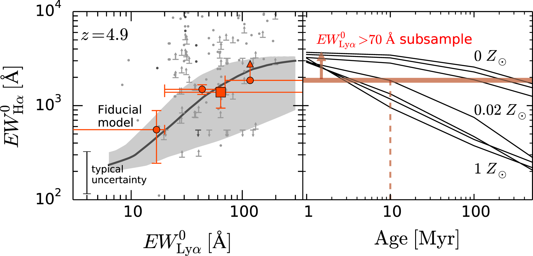
We thank the anonymous referee for a careful reading and valuable comments that improved the clarity of the paper. We are grateful to Richard Ellis, Anna Feltre, Max Gronke, Toshihiro Kawaguchi, Kimihiko Nakajima, Kazuhiro Shimasaku, and David Sobral for their useful comments and discussions. We thank Stefano Carniani for providing their data points.

The Hyper-Suprime-Cam (HSC) collaboration includes the astronomical communities of Japan and Taiwan, and Princeton University. The HSC instrumentation and software were developed by the National Astronomical Observatory of Japan (NAOJ), the Kavli Institute for the Physics and Mathematics of the Universe (Kavli IPMU), the University of Tokyo, the High Energy Accelerator Research Organization (KEK), the Academia Sinica Institute for Astronomy and Astrophysics in Taiwan (ASIAA), and Princeton University. Funding was contributed by the FIRST program from Japanese Cabinet Office, the Ministry of Education, Culture, Sports, Science and Technology (MEXT), the Japan Society for the Promotion of Science (JSPS), Japan Science and Technology Agency (JST), the Toray Science Foundation, NAOJ, Kavli IPMU, KEK, ASIAA, and Princeton University.

The Pan-STARRS1 Surveys (PS1) have been made possible through contributions of the Institute for Astronomy, the University of Hawaii, the Pan-STARRS Project Office, the Max-Planck Society and its participating institutes, the Max Planck Institute for Astronomy, Heidelberg, the Max Planck Institute for Extraterrestrial Physics, Garching, Johns Hopkins University, Durham University, the University of Edinburgh, Queen's University Belfast, the Harvard-Smithsonian Center for Astrophysics, the Las Cumbres Observatory Global Telescope Network Incorporated, the National Central University of Taiwan, the Space Telescope Science Institute, the National Aeronautics and Space Administration under grant no. NNX08AR22G issued through the Planetary Science Division of the NASA Science Mission Directorate, the National Science Foundation under grant no. AST-1238877, the University of Maryland, and Eotvos Lorand University (ELTE).

This paper makes use of software developed for the Large Synoptic Survey Telescope. We thank the LSST Project for making their code available as free software at http://dm.lsst.org.

This work is supported by World Premier International Research Center Initiative (WPI Initiative), MEXT, Japan, and KAKENHI (15H02064) Grant-in-Aid for Scientific Research (A) through Japan Society for the Promotion of Science (JSPS). Y.H. acknowledges support from the Advanced Leading Graduate Course for Photon Science (ALPS) grant and the JSPS through the JSPS Research Fellowship for Young Scientists. J.C. and S.C. acknowledge support from the European Research Council (ERC) via an Advanced Grant under grant agreement no. 321323-NEOGAL. S.T. acknowledge support from the ERC Consolidator Grant funding scheme (project ConTExt, grant No. 648179). The Cosmic Dawn Center is funded by the Danish National Research Foundation.

SILVERRUSH. V. Census of Lyα, [O iii] λ5007, Hα, and [C ii] 158 μm Line Emission with ∼1000 LAEs at z = 4.9–7.0 Revealed with Subaru/HSC

Article metrics

Permissions

Author e-mails

Author affiliations

Author notes

ORCID iDs

Dates

Abstract

1. Introduction

2. Sample

2.1. LAE Sample

2.2. [C ii] 158 μm Sample

3. Method

3.1. Removing Severely Blended Sources

3.2. Stacking Analysis

3.3. Model SED

3.4. Line Flux Estimate

4. Results

4.1. Properties of z = 4.9 LAEs

4.1.1. Inferred Hα EW

4.1.2. Lyα Escape Fraction

4.1.3. Ionizing Photon Production Efficiency

4.1.4. Ionizing Photon Escape Fraction

4.1.5. Star Formation Main Sequence

4.2. Properties of z = 5.7, 6.6, and 7.0 LAEs

4.2.1. [O iii] λ5007/Hα and [O iii] λ5007/Hβ Ratios

4.2.2. Metallicity–EW_Lyα Anticorrelation

4.3. [C ii] 158 μm–Lyα Relation

5. Discussion

5.1. Fiducial Model Reproducing the Lyα, [O iii], Hα, and [C ii]

5.2. Predicted C iii] λλ1907, 1909 EWs of LAEs

5.3. Implication for Cosmic Reionization

6. Summary

Footnotes

SILVERRUSH. V. Census of Lyα, [O iii] λ5007, Hα, and [C ii] 158 μm Line Emission with ∼1000 LAEs at z = 4.9–7.0 Revealed with Subaru/HSC

Article metrics

Permissions

Share this article

Author e-mails

Author affiliations

Author notes

ORCID iDs

Dates

Abstract

1. Introduction

2. Sample

2.1. LAE Sample

2.2. [C ii] 158 μm Sample

3. Method

3.1. Removing Severely Blended Sources

3.2. Stacking Analysis

3.3. Model SED

3.4. Line Flux Estimate

4. Results

4.1. Properties of z = 4.9 LAEs

4.1.1. Inferred Hα EW

4.1.2. Lyα Escape Fraction

4.1.3. Ionizing Photon Production Efficiency

4.1.4. Ionizing Photon Escape Fraction

4.1.5. Star Formation Main Sequence

4.2. Properties of z = 5.7, 6.6, and 7.0 LAEs

4.2.1. [O iii] λ5007/Hα and [O iii] λ5007/Hβ Ratios

4.2.2. Metallicity–EWLyα Anticorrelation

4.3. [C ii] 158 μm–Lyα Relation

5. Discussion

5.1. Fiducial Model Reproducing the Lyα, [O iii], Hα, and [C ii]

5.2. Predicted C iii] λλ1907, 1909 EWs of LAEs

5.3. Implication for Cosmic Reionization

6. Summary

Footnotes

4.2.2. Metallicity–EW_Lyα Anticorrelation