


Abstract
Solar magnetoseismology is an indirect method to approximate plasma parameters that are traditionally difficult to measure in the solar atmosphere using observations of magnetohydrodynamic waves. A magnetic slab can act as waveguide for magnetoacoustic waves that approximates magnetic structures in the solar atmosphere. The asymmetry of the slab caused by different plasma parameters in each external region affects both the eigenfrequencies and eigenfunctions differently at each side of the slab, that is, both the temporal and spatial profiles of the eigenmodes of propagation along the slab are influenced by the equilibrium asymmetry. We present two novel diagnostic tools for solar magnetoseismology that use this distortion to estimate the slab magnetic field strength using the spatial distribution of magnetoacoustic surface waves: the amplitude ratio and the minimum perturbation shift techniques. They have the potential to estimate background equilibrium parameters in inhomogeneous solar structures such as elongated magnetic bright points, prominences, and the clusters of magnetic brightenings rooted in sunspot light bridges known as light bridge surges or light walls, which may be locally approximated as slabs.
Export citation and abstract BibTeX RIS

Original content from this work may be used under the terms of the Creative Commons Attribution 3.0 licence. Any further distribution of this work must maintain attribution to the author(s) and the title of the work, journal citation and DOI.
1. Introduction
The emerging field of solar magnetoseismology (SMS) has become a crucial tool in developing our understanding of structures in the solar atmosphere. By comparing observational measurements of magnetohydrodynamic (MHD) waves to the wave solutions of inhomogeneous plasma modeling of the medium in which the waves propagate, we can make approximations of traditionally difficult-to-measure plasma parameters such as the magnetic field strength and heat transport coefficient (Andries et al. 2009; Arregui 2012; De Moortel & Nakariakov 2012). This in turn equips us with more realistic parameters for numerical simulations and gives us a better understanding of the conditions that lead to, for example, wave energy dissipation, instability, magnetic reconnection, and heating.
SMS techniques can be categorized as either temporal or spatial seismology. By temporal seismology we refer to methods that estimate a plasma parameter using the observed frequency, or equivalently the period, of waves. By spatial seismology we refer to methods that estimate a plasma parameter by comparing the observed spatial and/or temporal wave power distribution with the eigenfunctions from a theoretical model.
Several temporal seismology methods have been employed successfully. Rosenberg (1970) first suggested that the frequency of oscillations, observed through the fluctuation of synchrotron radiation due to the presence of MHD waves, could be used to diagnose background parameters. Further theoretical development has led to more sophisticated temporal methods including local coronal magnetic field strength estimates using standing kink modes in coronal loops by Nakariakov & Ofman (2001), and using slow sausage and kink modes by Erdélyi & Taroyan (2008). The ratio of periods of the fundamental and the first harmonic standing kink mode and its dependence on density stratification has also been well studied (Banerjee et al. 2007; Erdélyi et al. 2014; Yu et al. 2016).
Spatial seismology techniques have more recently started demonstrating their efficacy in estimating solar parameters. Uchida (1970) estimated the coronal magnetic structure by comparing Moreton wave observations with the theoretical influence that the coronal magnetic field has on the shape of the Moreton wavefront. More recent eigenfunction methods include utilizing the anti-node shift of standing modes in a magnetic flux tube to diagnose its inhomogeneous density stratification (Erdélyi & Verth 2007; Verth et al. 2007; Erdélyi et al. 2014).
In the present work, we derive two novel analytical tools for spatial seismology that use an asymmetric slab waveguide to approximate background parameters. This has applications to solar atmospheric structures that are locally slab-like, which have been observed to guide MHD oscillations, such as elongated magnetic bright points (MBPs; Yuan et al. 2014), prominences (Arregui et al. 2012), and light bridge surges (Roy 1973; Shimizu et al. 2009; which have also been named light walls by, e.g., Yang et al. 2015, 2017; Zhang et al. 2017).
This work provides an application of the linear wave analysis of asymmetric magnetic slabs completed by Allcock & Erdélyi (2017). A magnetic slab, with non-magnetic, but asymmetric density and temperatures outside the slab, has eigenmodes which can be described as either quasi-sausage or quasi-kink. For quasi-sausage (quasi-kink) modes, the oscillations on each slab interface are in anti-phase (phase). They differ in character from traditional (symmetric) sausage and kink modes by their asymmetry about the center of the slab due to the amplitude of oscillation on each interface being unequal caused by the asymmetric external environment. This results in quasi-kink modes not necessarily retaining their cross-sectional area and quasi-sausage modes not necessarily having reflection symmetric about the center line of the slab. The spatial distribution of these waves across the slab, and therefore the extent to which they are modified from the traditional sausage and kink modes, is dependent on the asymmetric background plasma parameters. Consequently, we can use the spatial distribution of these waves to diagnose the waveguide. This is the focus of the present paper: to derive expressions for proxy parameters that encapsulate this asymmetric spatial distribution and discuss the application to SMS.
Section 2 introduces the amplitude ratio diagnostic parameter, Section 3 introduces the minimum perturbation shift diagnostic parameter, and Section 4 discusses the application of these parameters to SMS.
2. Amplitude Ratio
The aim of this section is to derive an expression for the ratio of the oscillation on each interface of an asymmetric magnetic slab in terms of the wave and plasma parameters of the system.
Consider an inviscid plasma structured by two parallel interfaces separating the plasma into three regions along the  -direction. In each region the plasma is uniform and the central region, known as the slab, has a uniform magnetic field,
  . The plasma adjacent to the slab on each side is non-magnetic. The density, pressure, and sound speed within the slab are denoted by ρ0, p0, and c0, respectively, and in the external plasma they are subscripted by 1 and 2, respectively. The same equilibrium conditions were used, with more information given, by Allcock & Erdélyi (2017).
In the aforementioned work, it was shown that trapped magnetoacoustic modes propagating along an asymmetric magnetic slab have velocity perturbation in the  -direction given by
  , where ω and k are the angular frequency and wavenumber, and
where

and A, B, C, and D are arbitrary constants (with respect to x). These constants can be determined, to within one degree of freedom, using the boundary conditions of continuity in total (kinetic plus magnetic) pressure and transversal velocity component across the slab boundaries at x = ± x0. Applying these four boundary conditions retrieves four coupled linear homogeneous algebraic equations in the four unknowns:
where
and  and
and  for i = 0, 1, 2. Ensuring that this matrix has a vanishing determinant gives us the dispersion relation:
More information regarding the above derivation can be found in Allcock & Erdélyi (2017). By satisfying this relation, we gain one degree of freedom in the system of Equations (2.4), which leaves one of the constants B or C arbitrary. This gives us two types of solution: quasi-sausage and quasi-kink modes.
First, for quasi-sausage modes, by letting C be arbitrary the other constants A, B, and D can be determined as


where

The second formulation of B in Equation (2.9) is found by utilizing the dispersion relation. A substitution of these values, using the first form of B in Equation (2.9), into the velocity solution, Equation (2.1), evaluated at the slab boundaries, yields
where  . similarly, using the second form of B in Equation (2.9) yields

These forms are equivalent. The horizontal velocity perturbation amplitude,  , is the signed amplitude, where a positive (negative) value indicates perturbation in the positive (negative)
  -direction.
Second, for quasi-kink modes, by letting B be arbitrary, the other constants A, C, and D can be determined in terms of B as


where

A substitution of these values, using the first form of C in Equation (2.16), into (2.1), evaluated at the slab boundaries ( ), yields

Using the second form of C in Equation (2.16) yields


We now define the amplitude ratio,  , as the ratio of the amplitude of oscillation of the left interface (x = x0) to that of the right interface (x = −x0) (see Figure 1). Given that
  , we also have
  . First, using Equations (2.11) and (2.12), the amplitude ratio for quasi-sausage modes is
Using Equations (2.18) and (2.19), the corresponding expression for quasi-kink modes can be obtained, namely
As expected, Equations (2.21) and (2.22) reduce to  and
and  for sausage and kink modes, respectively, when the slab is symmetric.
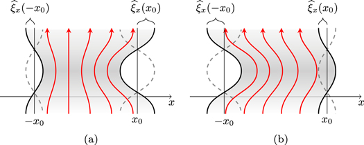
Figure 1. Illustration of the difference in amplitude of oscillation on each boundary of the slab for (a) quasi-sausage and (b) quasi-kink modes.
Download figure:
Standard image High-resolution imageThe following subsections give the analytical solution for the Alfvén speed,  , of Equations (2.21) and (2.22) under the thin slab, wide slab, incompressible plasma, and low-beta approximations. To obtain an approximation for the Alfvén speed analytically, an approximation such as these must be applied. Note that we restrict the analysis to surface modes only, thereby omitting body modes, because the eigenfrequencies and eigenfunctions of body modes are not significantly affected by asymmetry in the external plasma (Allcock & Erdélyi 2017).
2.1. Thin Slab Approximation
In the thin slab approximation,  , it has been shown that
  for surface modes (Roberts 1981b). Therefore,
  and the amplitude ratio for a quasi-sausage surface mode in a thin slab reduces to
which yields the analytical expression
The amplitude ratio for a thin slab quasi-kink surface mode reduces to
which yields the analytical expression
In a thin asymmetric slab, the fast quasi-kink surface mode degenerates due to a cutoff by the external sound speeds becoming distinct (Allcock & Erdélyi 2017) and the slow quasi-kink surface mode has a phase speed that approaches zero in the thin slab limit. Therefore, to a good approximation, the phase speed is much less than the internal sound speed ( ); therefore Equation (2.26) simplifies to
2.2. Wide Slab Approximation
The wide slab approximation applies when the slab width is much larger than the wavelength, that is when  . To understand the properties of the eigenfunctions of the asymmetric slab system in the wide slab approximation, we must return to the dispersion relation, Equation (2.6). For surface modes in the slab, the wide slab approximation implies that
  , therefore
  (Roberts 1981b). Under this approximation, the dispersion relation, Equation (2.6), becomes

which gives us two families of solutions, one satisfying  and the other satisfying
  . These are equivalent to

for j = 1, 2, respectively. This equation is the same as the dispersion relation governing surface waves along a single interface between a magnetized and a non-magnetized plasma (Roberts 1981a). Hence, the surface mode solutions of a wide asymmetric slab are just the surface modes that propagate along each interface independently. This again makes intuitive sense considering that as the slab is widened the interfaces will have diminishing influence on each other, until each interface oscillates independently with its own characteristic frequency.
This is analogous to the mechanical example introduced by Allcock & Erdélyi (2017). Consider two masses connected by a spring, with spring constant k0, and each mass is also connected to a fixed wall on each side by springs with spring constants k1 and k2, respectively (see Figure 2). When the middle spring has a spring constant  , there are two modes, an in-phase mode (analogous to kink modes in a slab) and an in-anti-phase mode (analogous to sausage modes in a slab). When the two masses are decoupled by removing the middle spring, equivalently setting k0 = 0, each mass oscillates independently at the natural frequency of that side of the spring-mass system. This decoupling provides a good analogy to the wide slab limit for the magnetic slab. Each interface can oscillate at its own natural frequency, independent of the other interface. Given that we are considering magnetoacoustic waves, there are two restoring forces, the magnetic tension force and the pressure gradient force, which means that each independent interface has two natural frequencies (depending on the parameters of the system, there can be 0, 1, or 2 frequencies), corresponding to the fast and slow magnetoacoustic modes. With this understanding of the modes in the wide slab limit, the amplitude ratio,
  , is either 0 or undefined, depending on which interface the wave is propagating and is therefore not useful for magnetoseismology.
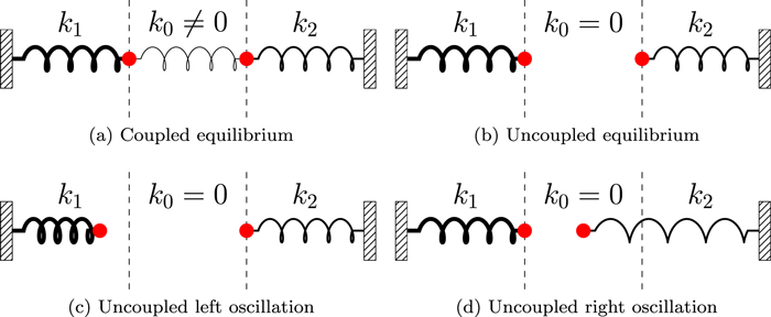
Figure 2. Mechanical example showing weak and zero coupling between the masses. This provides an analogy to the wide slab approximation of an asymmetric magnetic slab, in which case the interfaces on each side of the slab oscillate independently.
Download figure:
Standard image High-resolution image2.3. Incompressible Approximation
If the plasma is incompressible, the sound speeds become unbounded, so that mj ≈ k for j = 0, 1, 2. Under this approximation, the amplitude ratio for quasi-sausage modes (top) and quasi-kink modes (bottom) reduces to
These equations have solutions for  given by
2.4. Low-beta Approximation
For a low-beta plasma ( ), where the magnetic pressure dominates the kinetic plasma pressure, the Alfvén speed, vA, dominates the internal sound speed, c0, so that
  . For waves with phase speeds much less than the Alfvén speed, a further approximation of
  can be made, in which case the amplitude ratio for quasi-sausage modes (top) and quasi-kink modes (bottom) reduces to
These equations will provide for vA to give
We will return to a discussion of the inversion of the amplitude ratio in Section 4.
3. Minimum Perturbation Shift
A second spatial seismology technique uses the shift in the position of minimum wave power from the center of the slab due to the asymmetry in the external plasma regions as a diagnostic parameter for the slab Alfvén speed.
The position of minimum wave power for a symmetric sausage or kink mode is at the central line of the slab, at x = 0. We define Δmin to be the displacement (from the central line) of the position of minimum wave power inside an asymmetric magnetic slab (see Figure 3). For quasi-sausage modes, Δmin is the solution to  under the constraint
  , and for quasi-kink modes, Δmin is the solution to
  under the same constraint
  . The constraint restricts the solutions to being within the slab.
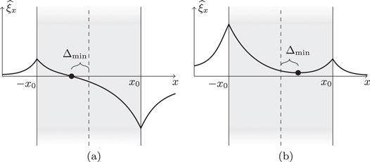
Figure 3. Illustration of the minimum perturbation shift, Δmin, within the slab (shaded) for (a) quasi-sausage and (b) quasi-kink modes.
Download figure:
Standard image High-resolution imageFirst, for quasi-sausage modes, using the solution for the transversal velocity amplitude given by Equation (2.1) and the expressions for the variables within given by Equation (2.9), the minimum perturbation shift can be calculated as follows. The solution for the transversal velocity amplitude within the slab is

where B is given by Equation (2.9) and C is arbitrary. This equation is solved for x to give

Therefore, the minimum perturbation shift for quasi-sausage modes is
Similarly, for quasi-kink modes, using Equations (2.1) and (2.16) we calculate the minimum perturbation shift to be

The dependence of expressions (3.3) and (3.4) for the minimum perturbation shifts on the external plasma with subscript 2 is implicit in the determination of the eigenfrequency ω when solving the dispersion relation.
The concept of minimum perturbation shift is exclusive to surface modes. The eigenfunctions of surface modes in a magnetic slab are significantly more sensitive to the external plasma parameters than body modes (Allcock & Erdélyi 2017). This makes intuitive sense given that the energy in a surface mode is localized to the boundaries of the slab, whereas the energy in a body mode is largely isolated within the slab. There is a shift in the spatial nodes and anti-nodes in body mode perturbations within a slab due to changing external plasma parameters, however, it is too small to be an effective observational tool.
Akin to the amplitude ratio method for solar magnetoseismology prescribed in Section 2, we can determine from Equation (3.3) or (3.4) the Alfvén speed, vA, to estimate the magnetic field strength of inhomogeneous solar magnetic structures. This can be done either numerically, using an iterative root finding method, or analytically, under an appropriate approximation. In each of the following subsections, we carry out an inversion for the Alfvén speed, vA, under a specific approximation.
3.1. Thin Slab Approximation
In Section 2.1, we addressed that under the thin slab approximation, that is  , we have
  for surface modes. This means that by definition
  , therefore
  , so
, so  . First, for quasi-sausage modes, Equation (3.3) can be solved for vA to give
For quasi-kink modes in a thin slab, Equation (3.4) can be solved for  to give
where


3.2. Wide Slab Approximation
The concept of minimum perturbation shift is ill-defined under the wide slab approximation, that is, when  . In this case, each interface oscillates independently at its own eigenfrequency. Therefore, the nomenclature of quasi-sausage and quasi-kink mode breaks down. In the wide slab limit, the eigenfunctions have no local minimum in the slab; instead the perturbations are evanescent away from the oscillating interface, therefore there is no local minimum of wave power within the slab.
3.3. Incompressible Approximation
When the plasma is incompressible, the sound speeds are unbounded, so that  , for j = 0, 1, 2. The minimum perturbation shift for a quasi-sausage mode (top) and quasi-kink (bottom) in an incompressible slab is
which yields for vA the expression
3.4. Low-beta Approximation
In a low-beta plasma, the minimum perturbation shift for a quasi-sausage mode (top) and quasi-kink (bottom) is given by
which provides for vA to give
4. Discussion
We have introduced the amplitude ratio and the minimum perturbation shift, which quantify the spatial asymmetry in magnetic slab eigenmodes. These expressions can be applied to determine the Alfvén speed, for a given set of observed equilibrium parameters, providing us a novel method to diagnose information about the background plasma, thus advancing the field of spatial magnetoseismology.
A summary of the analytical expressions for estimating the Alfvén speed, vA, within an asymmetric magnetic slab, is given in Tables 1 and 2, utilizing the amplitude method and the minimum perturbation shift methods, respectively. In practice, a numerical procedure could be made relatively simple and computationally inexpensive by making use of a standard root finding method once the observed parameters have been prescribed, but in some cases it might be valid to use an analytical solution from Tables 1 and 2 under the necessary approximation.
Table 1. Magnetoseismology Application Using the Amplitude Ratio, RA, to Approximate the Alfvén Speed, vA
| Mode | Approximation of  Using the Amplitude Ratio, RA Using the Amplitude Ratio, RA |
||
|---|---|---|---|
| Thin slab | Incompressible | Low-beta | |
| Quasi-sausage Surface |
|
|
|
| Quasi-kink Surface |
|
|
|
Download table as: ASCIITypeset image
Table 2. Magnetoseismology Application Using the Minimum Perturbation Shift, Δmin, to Approximate the Alfvén Speed, vA
| Mode | Approximation of  Using the Minimum Perturbation Shift, Δmin Using the Minimum Perturbation Shift, Δmin |
||
|---|---|---|---|
| Thin slab | Incompressible | Low-beta | |
| Quasi-sausage Surface |
|

|
|
| Quasi-kink Surface |
 , defined in Section 3.1 , defined in Section 3.1
|
|
|
Download table as: ASCIITypeset image
Figure 4 illustrates the dependency of the amplitude ratio and minimum perturbation shift on the (non-dimensionalized) slab width, kx0, and the density ratio, ρ1/ρ0, of one external plasma density to the slab density, holding the other external density fixed. Varying one density ratio in this way is equivalent to changing the asymmetry of the system. The amplitude ratio is positive (negative) for quasi-kink (quasi-sausage) modes, because the oscillations on each boundary are in-phase (anti-phase). Figures 4(a) and (b) further show that, for a given background parameter regime, the boundary with the highest amplitude is different for quasi-kink and quasi-sausage modes. This is demonstrated by the absolute value of the amplitude ratio being greater than 1 for quasi-sausage modes when it is less than 1 for quasi-kink modes, and vice versa. This is in agreement with the properties of the eigenmodes of the analogous spring-mass system introduced by Allcock & Erdélyi (2017). Figures 4(c) and (d) demonstrate that the position of minimum perturbation for quasi-kink modes is shifted in the opposite direction to that of quasi-sausage modes.
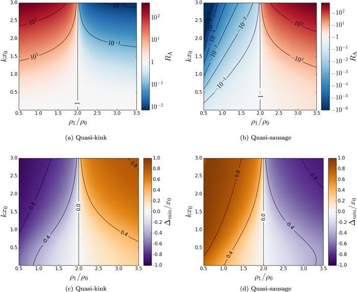
Figure 4. (a), (b) The amplitude ratio, RA, and (c), (d) the minimum perturbation shift, Δmin, as a function of the slab width, non-dimensionalized to kx0, and the density ratio, ρ1/ρ0, for slow (a), (c) quasi-kink and (b), (d) quasi-sausage surface modes. The other density ratio is set to ρ2/ρ0 = 2, the characteristic speed ordering inside the slab is vA = 1.3c0, and the sound speed outside the slab is determined to ensure equilibrium pressure balance.
Download figure:
Standard image High-resolution imageThere are a number of ways that the amplitude ratio or minimum perturbation shift can be used for spatial seismology. For a given observed wave event in a slab-like solar atmospheric structure, the most simple procedure is as follows. Take measurements for the wave parameters (period and wavelength), and the background parameters (width of structure, plasma density in each region). Determine the sound speeds by assuming equilibrium pressure balance across the slab boundaries. Take a measurement of either the amplitude ratio or minimum perturbation shift. Then invert the corresponding expression for the spatial wave distribution parameter, Equations (2.21), (2.22), (3.3), or (3.4), to estimate the Alfvén speed.
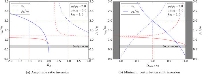
However, it is often the case that not all the non-magnetic parameters characterizing a waveguide are well-observable. In this case, the dispersion relation can be solved simultaneously with the equation for the amplitude ratio or the minimum perturbation shift to approximate the Alfvén speed and another unknown parameter. For example, Figure 5 shows the inversion curves for a particular parameter regime typical of a slow surface mode. It is plotted by prescribing (as if they were observed quantities) all plasma parameters except the Alfvén speed, vA, and one of the density ratios, ρ1/ρ0, then simultaneously solving the dispersion relation, Equation (2.6), with the expressions for the amplitude ratio, Equation (2.21) or (2.22), or the minimum perturbation shift, Equation (3.3) or (3.4). The solution curves were found numerically.
Figure 5. Using prescribed values for (a) the amplitude ratio, RA, or (b) the minimum perturbation shift, Δmin, a numerical inversion is used to approximate the background equilibrium parameters, in this case the Alfvén speed, vA, and one of the density ratios, ρ1/ρ0, for slow magnetoacoustic modes. The dashed (solid) lines correspond to the inversion curves for slow quasi-kink (quasi-sausage) surface modes. The dotted lines indicate the inversion for symmetric kink and sausage modes. The light-shaded area indicates the values of the Alfvén speed, which correspond to body modes rather than surface modes, and so are not important for SMS application. The dark shaded region in Figure (b) illustrates the region outside the slab, outside the bounds of the minimum perturbation shift.
Download figure:
Standard image High-resolution image
Plasma density measurements often have low accuracy and large uncertainty. These uncertainties will propagate through the inversion of the amplitude ratio or minimum perturbation shift to lead to uncertainties in the diagnosis of the Alfvén speed. Measuring the density ratio is likely to be the source of the largest uncertainty in the estimation, since errors in spatial parameters such as the half slab width, x0, and temporal parameters, such as the angular frequency, ω, are generally much smaller. The propagation of the error in the density ratios is reduced by a factor of two by the square root that is introduced when inverting vA from k2vA2/ω2 (in a similar way to Nakariakov & Ofman 2001). Furthermore, by following the numerical approach described in the previous paragraph, measurement of only one of the density ratios is necessary to estimate the Alfvén speed. Therefore, combined with high-precision methods using density-sensitive emission lines (Young et al. 2009), the propagation of density measurement errors can be reduced.
The amplitude ratio has a strong sensitivity to the changes in the external densities, and therefore the external asymmetry, whereas the minimum perturbation shift has a weaker dependency. Therefore, the amplitude ratio is likely to be a more effective parameter for diagnosing background parameters. Furthermore, observations of the location of the minimum wave power within a solar magnetic slab will be fraught with noise, potentially causing the detection of a false minimum. Noise in amplitude ratio measurements is less likely to introduce large errors because the locations of the slab boundaries are a more obvious features and can be identified by the steep gradients in the wavelength of observed light, for example, and is stable to larger noise signals.
Both the amplitude ratio and minimum perturbation shift are more sensitive to small changes in the background equilibrium parameters, i.e., the asymmetry in the background plasma, than the eigenfrequencies are. On a theoretical level, this corroborates with the result that eigenfunctions of linear operators on a Hilbert space are often more sensitive to small perturbations of the operator than their corresponding eigenvalues (Kato 1995). The amplitude ratio and minimum perturbation shift both depend on the eigenfunctions,  , and their eigenvalues, ω2. This means that spatial seismology techniques can be theoretically more effective than temporal techniques for many solar structures. Therefore, we are excited to see a push for increased spatial resolution with next-generational observational instrumentation such as the Daniel K. Inouye Solar Telescope (DKIST). Upon completion, this will equip us to be able to use the magnetoseismology techniques developed here to better understand the diagnostic properties of asymmetric slab-like solar atmospheric structures such as elongated MBPs, prominences, and sunspot light walls.
Large MBPs, with characteristic length L > 500 km, along intergranular lanes are often rather elongated (Crockett et al. 2010). The application of SMS techniques to MBPs is limited by the low spatial resolution of current observations. DKIST is going to have a spatial resolution of 19 km for structures on the solar surface (Tritschler et al. 2015), sufficient enough to resolve oscillations in MBPs. This unprecedented resolution will hopefully give the sufficient number of pixels (5–10) across an MBP to determine whether their oscillations have maximum power at the boundaries of or within the waveguide, that is, to differentiate between the transverse eigenfunctions of surface and body MHD modes, respectively. This is crucial for the accurate employment of these SMS techniques, and would build upon previous work on mode identification such as the surface modes that were identified in photospheric pores (Moreels et al. 2015).
Quiescent prominences, which are large long-lived magnetic formations of cool dense plasma elevated into the hot and rarefied coronal atmosphere, can be approximated by magnetic slabs and have been regularly observed to guide MHD waves (Arregui et al. 2012). The basic slab model of prominences, as illustrated by, e.g., Joarder & Roberts (1992a, 1992b), is of a symmetric slab; however, a small asymmetry could easily be caused by adjacent inhomogeneities. Even a small asymmetry in density ( ) can cause a significant (factor of 2 or more) asymmetry in the eigenmode (Figure 4), except for in thin slabs. This makes prominences a good candidate for applying the SMS techniques developed here. One issue that one has to bear in mind for the employment of these techniques is that the approximation of simple asymmetric magnetic slab may be insufficient to capture some important aspects of prominence oscillations, in particular, prominences are likely to have a sheared magnetic field and may have significant flows, which are neglected in the asymmetric slab model (van Ballegooijen & Martens 1989; Zirker et al. 1994; Ballester 2005; Oliver 2009; Arregui et al. 2012).
Light bridge surges also present a possible application for the SMS techniques developed here. Rooted in sunspot light bridges, these clusters of recurrent chromospheric surges (observed as bright structures in, e.g., IRIS 1330 Å line, as observed by Yang et al. 2016) are formed by either magnetic reconnection just above the light bridge (Toriumi et al. 2015; Robustini et al. 2016) or by leakage of p-modes from beneath the underlying photosphere (Yang et al. 2015; Zhang et al. 2017). They have been demonstrated to guide MHD waves driven by nearby disturbances (Yang et al. 2016, 2017). While the asymmetric magnetic slab could be a valid approximation for the actual geometry of light walls, the strong magnetic field in the low solar atmosphere above a sunspot umbra (the plasma on each side of the light bridge) may put into question the full validity of the non-magnetic external plasma in the current model. However, what matters is the relative strength of the magnetic force compared to the pressure gradient force, that is, the value of plasma-beta. The value of beta above magnetic pores and sunspots is uncertain, but has been shown to be rather high in some cases (Bourdin 2017), and has therefore been used in models of the low atmosphere (Mumford et al. 2015). With improved observations, it may turn out that the plasma surrounding light walls has a low-beta, in which case we suggest a future generalization of the methods described here that involves an asymmetric magnetic plasma outside the slab will be a more appropriate method for the first magnetoseismology diagnosis of sunspot light walls.
Of course, these methods have limited applications due to the fact that we have modeled the slab as infinitely long and there do not exist any infinitely long waveguides in the solar atmosphere. However, if the length, L, of the cross section of an observed solar waveguide is much greater than its width, x0, say L/x0 = 5–10, then this model of an infinitely long slab may be a valid approximation. Furthermore, if the wavelength of the observed wave, λ, is such that  , then the thin slab approximation holds (Sections 2.1 and 3.1), therefore an analytical diagnosis of the Alfvén speed within the waveguide can be made using Table 1 or 2.
This paper introduces two novel SMS methods that, for the first time, explore the asymmetry of solar magnetic waveguides to diagnose background parameters. While the simplicity of the current model of an infinitely long slab in a non-magnetic environment introduces several problems for applying the methods, the focus is on the novel concept of waveguide asymmetry. Future advancements of these methods involving more complex equilibrium conditions will be valuable in the coming age of high-resolution solar observations. We propose to determine whether asymmetric magnetoacoustic surface waves can be excited within the characteristic lifetime of an asymmetric waveguide in the solar atmosphere. This task can be investigated analytically (for linear waves with simple initial conditions) and numerically (for nonlinear waves with more sophisticated initial conditions). Furthermore, a more realistic system, in particular, asymmetric magnetic fields in the external plasmas (see Zsámberger et al. 2018), or an equilibrium shear flow, would allow for better application to the solar waveguides discussed above, at the expense of analytic tractability.
The authors thank the anonymous referee for the constructive comments. M. Allcock is thankful for the University Prize Scholarship from the University of Sheffield. R. Erdélyi acknowledges the support from the UK Science and Technology Facilities Council (STFC, grant number ST/M000826/1) and the Royal Society.