


Abstract
We provide the theoretical background for diagnostics of the thermal properties of solar prominences observed by the Atacama Large Millimeter/submillimeter Array (ALMA). To do this, we employ the 3D Whole-Prominence Fine Structure (WPFS) model that produces synthetic ALMA-like observations of a complex simulated prominence. We use synthetic observations derived at two different submillimeter/millimeter (SMM) wavelengths—one at a wavelength at which the simulated prominence is completely optically thin and another at a wavelength at which a significant portion of the simulated prominence is optically thick—as if these were the actual ALMA observations. This allows us to develop a technique for an analysis of the prominence plasma thermal properties from such a pair of simultaneous high-resolution ALMA observations. The 3D WPFS model also provides detailed information about the distribution of the kinetic temperature and the optical thickness along any line of sight. We can thus assess whether the measure of the kinetic temperature derived from observations accurately represents the actual kinetic temperature properties of the observed plasma. We demonstrate here that in a given pixel the optical thickness at the wavelength at which the prominence plasma is optically thick needs to be above unity or even larger to achieve a sufficient accuracy of the derived information about the kinetic temperature of the analyzed plasma. Information about the optical thickness cannot be directly discerned from observations at the SMM wavelengths alone. However, we show that a criterion that can identify those pixels in which the derived kinetic temperature values correspond well to the actual thermal properties in which the observed prominence can be established.
Export citation and abstract BibTeX RIS
1. Introduction
The cool and dense plasma of solar prominences is held within the significantly less dense corona by nearly horizontal magnetic fields, which also insulate the prominence from the much hotter coronal environment. The large-scale plasma structure of quiescent solar prominences remains rather stable for extended periods of time, ranging from several days to a few months (see, e.g., Vial & Engvold 2015). In contrast, prominence fine structures with dimensions of the order of 1000 km (or less, see e.g., Lin et al. 2005) exhibit highly dynamical behavior with significant variations on timescales of several minutes. Examples can be found in, e.g., Lin et al. (2007) or Berger et al. (2008).
Thermal properties of the prominence fine structure plasma are determined by the balance of energy supplied and released by a number of sources. Energy is supplied by irradiation from the solar surface and the surrounding prominence or coronal plasma, by thermal conduction along the magnetic field lines, and by enthalpy. Energy is lost mainly in the form of emitted radiation. The energy balance significantly influences the stability of the prominence plasma, and thus the life-time of the prominence fine structures. One of the crucial parameters needed for the study of the prominence energy balance is the kinetic temperature of the prominence plasma. The only information about the prominence plasma thermal properties that can be obtained is in the form of the observed radiation emerging from a prominence. To interpret observations obtained in the optical or UV spectral range one needs to employ sophisticated non-LTE (i.e., departures from Local Thermodynamic Equilibrium) radiative transfer modeling techniques. However, even when using such modeling, it is difficult to exactly derive the kinetic temperature because its effect on the emitted radiation is highly nonlinear and non-local (see e.g., Vial & Engvold 2015). Prominence modeling was reviewed by Gunár (2014) or in the book Solar Prominences (Vial & Engvold 2015). Reviews of the physics of solar prominences can also be found in Tandberg-Hanssen (1995), Labrosse et al. (2010), and Mackay et al. (2010), or in the proceedings of the IAU 300 Symposium (Schmieder et al. 2014). Observations of quiescent prominences were reviewed by Heinzel et al. (2008).
In contrast to the optical or UV observations, kinetic temperature can be derived more directly from radio observations (e.g., Loukitcheva et al. 2004; Heinzel & Avrett 2012). This can be achieved, for example, from two nearly simultaneous observations at submillimeter/millimeter (SMM) wavelengths, where, in one, the observed prominence plasma is optically thin and, in the other, it is optically thick. Another option is to derive kinetic temperature from a single observation at the SMM wavelengths and a simultaneous observation in a different spectral range, for example, in the Hα line (see Heinzel et al. 2015). Prominence radio observations were previously obtained using single-dish instruments delivering a moderate spatial resolution (see Bastian et al. 1993, Irimajiri et al. 1995, and Gopalswamy et al. 1998). Only in recent years have we started to have access to the higher resolution SMM observations thanks to the Atacama Large Millimeter/submillimeter Array (ALMA). Its ability to observe solar filaments and prominences was demonstrated during the science verification observations (https://almascience.eso.org/alma-data/science-verification), albeit still with limited spatial resolution. Better spatial resolution is expected from observations during recent observing cycles for which several proposals for prominence observations were accepted. The special solar observing mode of ALMA was described by Karlický et al. (2011) and the potential of the solar observations by ALMA was reviewed by Wedemeyer et al. (2016). The ALMA Sun observations employing the fast-scan single-dish mapping are described in White et al. (2017). The high-resolution interferometric imaging of the Sun with ALMA is detailed in Shimojo et al. (2017). The potential visibility of the prominence fine structures in the ALMA prominence observations was demonstrated by Heinzel et al. (2015) and Gunár et al. (2016). Heinzel et al. (2015) used coronagraphic prominence observations in the Hα line to derive the visibility of the cool prominence fine structures. Gunár et al. (2016)—hereafter, referred to as Paper I—used the 3D Whole-Prominence Fine Structure (WPFS) model of Gunár & Mackay (2015a) to construct the first synthetic high-resolution images of a simulated prominence. The 3D WPFS model is the first model that represents an entire prominence and describes in detail the temperature and pressure variations of the prominence plasma distributed along many hundreds of fine structures. The modeled prominence fine structure plasma is located in dips of the magnetic field configuration provided by nonlinear force-free field (NLFF) simulations of Mackay & van Ballegooijen (2009). These dips are filled with plasma using the method developed by Gunár et al. (2013). This combination of realistic simulations of the prominence magnetic field configuration and a detailed physical model of the prominence fine structure plasma currently produces the most comprehensive model of prominences. This was demonstrated by Gunár & Mackay (2016) who analyzed the physical properties of the magnetic field and plasma of the WPFS model. The 3D WPFS model is also able to produce prominence structures resembling those observed in the Hα line. This was demonstrated by Gunár & Mackay (2015a) and further by Gunár & Mackay (2015b) who studied the evolution of the modeled prominence fine structures due to changes in the underlying magnetic flux distribution.
The present paper aims to serve as a theoretical preparation for the interpretation and analysis of future ALMA prominence observations. In the absence of the actual ALMA observations, we use the synthetic observations provided by the 3D WPFS model. To achieve the highest accuracy of the derived information about the kinetic temperature of the analyzed prominence plasma, we use here a pair of synthetic observations in wavelengths from both edges of the full future spectral range of ALMA. The chosen wavelengths—0.45 mm (666 GHz) and 9.0 mm (33 GHz)—correspond to wavelengths used in Paper I. The wavelength of 0.45 mm (666 GHz) represents ALMA band 9 and the wavelength of 9.0 mm (33 GHz) represents band 1. The simulated prominence is completely optically thin at 0.45 mm, while its significant part is optically thick at 9.0 mm (see Figures 1 and 4 of Paper I). We note here that ALMA bands 9 and 1 are at the time of writing not available for the solar observations. During the last ALMA observing cycle, only bands 6 and 3 were available for observations of the Sun. We also note that the current status of the development of the band 1 indicates that it will reach a slightly shorter wavelength of 8.6 mm (35 GHz) instead of 9.0 mmm (33 GHz) used here. Moreover, ALMA band 10 will provide access to even shorter wavelengths than those covered by the band 9 assumed here.
The paper is organized as follows: In Section 2, we briefly summarize the main characteristics of the 3D WPFS model used to construct the synthetic observations. In Section 3, we describe the method used to derive information about the kinetic temperature from observations at the SMM wavelengths. In Section 4, we apply this method to high-resolution synthetic brightness temperature maps provided by the 3D WPFS model. In Section 5, we introduce the weighted-mean kinetic temperature that serves as a representative measure of the complex distribution of the kinetic temperature of the simulated prominence plasma. In Section 6, we assess the accuracy of the information about the kinetic temperature derived from observations. We do so by comparing it with the weighted-mean kinetic temperature. In Section 7, we describe the relationship between the optical thickness at the wavelength at which a significant part of the prominence is optically thick and the brightness temperature at the wavelength at which the prominence is completely optically thin. Section 8 provides the discussion and offers our conclusions.
2. Brief Description of the 3D WPFS Model
In this section, we summarize the aspects of the 3D WPFS model that are essential for a clear understanding of the results presented in this paper. In doing so, we refer to relevant publications and, where appropriate, specific equations and figures that can illustrate the described properties of the model.
The 3D WPFS model of Gunár & Mackay (2015a) represents an entire prominence with its numerous prominence fine structures located in a 3D magnetic field configuration provided by the NLFF simulations of Mackay & van Ballegooijen (2009). The simulated magnetic field configuration is composed of a magnetic arcade and an inserted bipole (see Mackay & van Ballegooijen 2009 and Gunár & Mackay 2016). The minority polarity of the bipole is advected toward the axis of the arcade field. The evolution of the whole magnetic field configuration is described by a series of quasi-static NLFF states. Details of the NLFF simulations and the evolution of the simulated magnetic field configuration can be found in Section 3 of Mackay & van Ballegooijen (2009) and in Section 2 of Gunár & Mackay (2015b).
The resulting prominence magnetic field configuration contains regions where the field is dipped. Gunár & Mackay (2015a see Section 3 therein) used a randomized selection method to identify all magnetic field lines that contain a dip. These field lines are plotted in Figure 3 of Gunár & Mackay (2015a) from both the top view (seen as a filament against the solar disk) and side views (seen as a prominence above the solar limb). Additional visualization of the used magnetic field configuration showing also the field strength can be found in Gunár & Mackay (2016). Each dipped field line accommodates an individual simulated prominence fine structure. The geometry of each fine structure (illustrated in Figure 4 of Gunár & Mackay 2015a) is the following: (i) we assume a circular cross-section with a radius of 500 km (i.e., a diameter of 1000 km) centered at the selected field line; (ii) magnetic field is assumed to be identical to the selected field line within this cross-section; (iii) the length of the fine structure depends on the depth of the magnetic dip and is determined by the method of Gunár et al. (2013). This method is used to populate magnetic dips with the prominence plasma (for more details, see Figure 2 of Gunár et al. 2013). Dips are iteratively filled by hydrostatic plasma with prescribed temperature distribution. A scheme of the filling method can be found in Figure 3 of Gunár et al. (2013).
The 3D WPFS model assumes a set of global input parameters that are identical for all modeled fine structures. A complete list of the global input parameters can be found in Table 1 of Gunár & Mackay (2015a). These parameters define, for example, the plasma temperature variation by setting the minimum temperature, maximum temperature, and temperature gradients. They also define the mass loading via the set boundary pressure and maximum column mass. In the present work, we use the same values of the global input parameters as those in Gunár & Mackay (2015a). It is important to note that even though the WPFS model uses such a set of global input parameters for all fine structures, individual fine structures are in essence unique. This is due to the fact that each modeled fine structure has, in general, a different shape of the dipped magnetic flux tube defined by the shape of the central field line. The temperature and the pressure variation of the prominence plasma in individual fine structures is dependent on the depth and the shape of the dipped field through the used hydrostatic equilibrium method of Gunár et al. (2013). This results in a difference of the plasma properties between individual modeled fine structures.
The plasma pressure along the selected central field line increases hydrostatically with the increasing depth of the dip (see Equation (5) of Gunár et al. 2013). The radially symmetric pressure variation within the fine structure cross-section is determined by the variation of the column-mass described by Equation (8) of Gunár et al. (2013). The resulting 3D distribution of the plasma pressure within a single simulated prominence fine structure can be seen in Figure 4 (panels c and d) of Gunár & Mackay (2016). The temperature variation of the fine structure plasma is prescribed semi-empirically to accommodate the transition region between the central cool prominence plasma and the surrounding hot corona—the so-called Prominence-Corona Transition Region (PCTR). We assume that each simulated fine structure has its own PCTR with two distinct shapes. Along the field lines, the temperature increases gradually from the minimum temperature in the center of the dip toward the maximum at its edges. This increase is prescribed by Equation (2) of Gunár et al. (2013). In the radial direction within the fine structure cross-section—i.e., in the direction perpendicular to the magnetic field—we assume a steep temperature gradient prescribed by Equation (7) of Gunár et al. (2013). The difference between these temperature gradients is due to the fact that the thermal conduction is significantly inhibited in the direction perpendicular to the magnetic field. The 3D distribution of the temperature within a single simulated fine structure can be seen in Figure 4 (panels a and b) of Gunár & Mackay (2016). A visualization of the 3D distribution of the temperature and pressure in the entire modeled prominence composed of over 800 fine structures can be seen in Figure 5 of Gunár & Mackay (2016).
The maximum temperature in the WPFS model assumed in the present work is 100,000 K. This value is set as one of the global input parameters and defines the PCTR temperature at the outer edges of the simulated prominence fine structures. However, the temperature within the PCTR in prominences is expected to reach up to the coronal values. Whether it reaches those values in between individual fine structures or only within the region enveloping entire prominences is not fully known. This issue was discussed, for example, by Gunár et al. (2014 see Section 6.1 therein). However, the plasma contained in the space between the cool prominence fine structures does not significantly contribute to the specific intensity of radiation at the SMM wavelengths. This is due to the fact that the plasma pressure in between fine structures is significantly lower than inside them (in the present work, we assume the coronal pressure values). Moreover, the specific intensity at the SMM wavelengths is in fact proportional to T−1/2. This means that the intensity decreases with the increasing temperature—for more details, see the discussion in Section 5.1 of Paper I. Therefore, the space between the modeled fine structures is not relevant to the results of the present work.
3. How to Derive Kinetic Temperature from Observed Brightness Temperature
The specific intensity of radiation emerging from a prominence at the limb at the SMM wavelengths is determined by the fact that the source function is equal to the Planck function Bν(T) for the blackbody radiation (see, e.g., Heinzel et al. 2015; Gunár et al. 2016). Thus we can write for the specific intensity

where the increment to the optical depth dtν = κν dl, τν represents the total optical depth along a geometrical path with a length L, and κν is the absorption coefficient (for more details see, e.g., Rybicki & Lightman 1979, Heinzel et al. 2015, or Paper I).
At the SMM wavelengths, the Planck function is directly proportional to the local kinetic temperature T as

and the specific intensity Iν is directly proportional to the brightness temperature Tb (see, e.g., Rybicki & Lightman 1979) as

We can thus rewrite Equation (1) as

If we assume a constant kinetic temperature T along the line of sight (LOS), we get

The assumption of a constant kinetic temperature of the prominence plasma may be relatively unrealistic. However, such an approximation is the only information about the thermal conditions of observed prominences that can be derived directly from observations at the SMM radio domain. In the present work, we analyze the relation between the representation of the kinetic temperature conditions of the prominence plasma derived from observations (Tk_der) and the distribution of the actual kinetic temperature within the prominence plasma.
To obtain Tk_der, a pair of observations of the same plasma at different wavelengths is needed. These wavelengths may be a pair of SMM wavelengths, where, in one, the observed plasma is optically thin, and, in the other, it is optically thick.
For the wavelength, where the plasma is optically thick, we can rewrite Equation (5) into the form

where  is the observable.
In the case where plasma is optically thin, we have

where  is the observable.
The optical depth τν along a geometrical path with a total length L is defined as

The absorption coefficient κν in the SMM domain can be written as

Here ne and np represent the electron and proton densities, respectively. We assume α = 0.018 gff and the Gaunt factor gff to be unity. For more details, see Paper I or Heinzel et al. (2015). Additional details can be found in Bastian et al. (1993), Irimajiri et al. (1995), Gopalswamy et al. (1998), or Loukitcheva et al. (2004). As follows from Equations (8) and (9), the ratio of the optical depths at different SMM frequencies (wavelengths), where one represents an optically thin prominence plasma emission and the other optically thick emission, can be expressed as

Using Equations (7) and (10), we can rewrite Equation (6) as
By solving this equation numerically, we can derive a quantity Tk_der from two observables  and
and  . In the following sections, we show how well such derived Tk_der represents the actual conditions of the prominence plasma with its significantly varying temperature.
4. Tk_der Derived from Synthetic Brightness Temperature Maps
To obtain Tk_der, we use a pair of synthetic ALMA brightness temperature maps provided by the 3D WPFS model. We use these maps as if they were a pair of actual ALMA observations. The technique used to produce these synthetic Tb maps is described in detail in Paper I. The method for derivation of Tk_der described in the previous section produces the most accurate results when, in one wavelength, the observed prominence plasma is completely optically thin and, in the other, it is optically thick. To ensure that the largest possible part of the simulated prominence is optically thick, we use here a synthetic Tb map at the 9.0 mm wavelength (see the optical thickness map in Figure 4 of Paper I). This wavelength is at the limit of (or perhaps even slightly beyond) the currently projected ALMA spectral range. We note that a shorter wavelength would produce similar results, but with larger uncertainties in pixels where the prominence plasma would not remain sufficiently optically thick. In the other used wavelength (0.45 mm) the entire simulated prominence is completely optically thin, as can be seen from the optical thickness map in Figure 1 of Paper I.
The used synthetic brightness temperature maps ( and
and  ) have a resolution of 150 × 150 km and contain over 50,000 synthetic pixels each. The 3D WPFS model producing these synthetic observations contains a large number of individual fine structures (over 800) which have, in essence, unique compositions of the plasma properties—see Section 2. Moreover, these fine structures are arranged stochastically, following the structure of the magnetic field of the modeled prominence. These facts mean that the synthetic observations used here represent sufficiently large and heterogeneous data sets, which are suitable for a statistical analysis.
At this point, we need to acknowledge that synthetic observations, such as those used in the present paper, are model dependent. First, they depend on the prominence model used to provide the physical representation of the simulated prominence plasma. Second, they depend on the choice of the parameters of the applied model. Third, synthetic observations depend on the accuracy of the method used to produce them. The 3D WPFS model applied here is the only model that provides a simulated prominence environment with the entire prominence consisting of a large number of fine structures in a 3D geometry with a high spatial resolution. As such, it is the first model that can be used for a qualitative analysis, as performed in the present paper. The method we use for the synthesis of the SMM emission from the simulated prominence plasma is described in detail in Paper I. This method is based on realistic assumptions and proven radiative transfer techniques for the synthesis of the SMM radio continua. The dependence of the synthetic observations on the model parameters is, for the case of the 3D WPFS model used here, not very significant. We take this fact into account in Section 7.
By numerically solving Equation (11) in each pixel in the synthetic observations at 0.45 and 9.0 mm wavelengths, we obtain  for each pixel. However, not all of the derived values of
  are accurately representing the thermal conditions of the plasma distributed along lines of sight passing through individual pixels. This is due to the fact that we cannot expect that the observed prominence will be optically thick (i.e., have optical thickness above unity) in all pixels, even at the 9.0 mm wavelength. This can be clearly seen in the optical thickness map in Figure 4 of Paper I, where large parts of the modeled prominence have τ9.0 < 1. The same can be true for any observed prominence. Thus, without the added information about the actual optical thickness—in our case, provided by the model—the derived values of Tk_der cannot be automatically assumed to be accurate in all pixels. This inaccuracy stems from the fact that in the pixels where the optical thickness is not large enough (around unity or higher) the basic approximation of the method used to derive Tk_der (Section 3) is not fulfilled. The magnitude of this inaccuracy can be discerned from the distribution of the derived
  values plotted in panels (a) and (b) in Figure 1. In these panels, we show, respectively, scatter plots of
  and
and  with respect to
  . From these scatter plots it is apparent that for larger values of the brightness temperature, the derived
  values cluster between 8000 and 11,000 K. However, for smaller Tb, the spread of
  is very large.
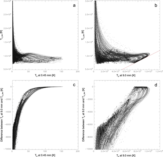
Figure 1. Scatter plots in panels (a) and (b) show distribution of the derived  values plotted with respect to the brightness temperature at 0.45 mm and 9.0 mm, respectively. Scatter plots in panels (c) and (d) show the difference between values of the brightness temperature at 9.0 mm and the derived
  , again with respect to the brightness temperature at 0.45 and 9.0 mm.
Download figure:
Standard image High-resolution imageThe most interesting feature that can be identified in the scatter plot in panel (b) is an area where the data points cluster along a linear feature highlighted by the drawn red dashed line. In these pixels, the derived  is equal to the observed
  . From Equation (6), it is clear that such a situation arises when τ9.0 would be around 4 or higher (for τ = 4 one obtains
  ). Therefore, in pixels where
  the derived values of
  do represent the thermal properties of the plasma distributed along the LOS corresponding to the given pixel. For an analysis of how well Tk_der represents the actual kinetic, see Section 6. While this is possible in synthetic observations, in the actual ALMA observations it may be difficult to reliably identify such linear features indicating pixels where
  . The synthetic observations used here are by design co-spatial, co-temporal, have exactly the same resolution, and each pixel obtained at any wavelength corresponds to exactly the same plasma. This will not be the case for the real observations. The uncertainties in the coalignment of the real observations due to the different resolution of the data obtained at different wavelengths and any noise in the observed data will lead to additional dispersion of the points in scatter plots such as those in Figure 1. Such dispersion can easily mask any linear features. Moreover, such an identification may become even more difficult if only a small number of pixels is obtained.
More importantly, even in the case when it is possible to identify pixels where  , a large majority of the observed pixels would be excluded from the analysis, if only those pixels where
  were taken into account. However, a large number of pixels where the optical thickness is less than 4 but still significant (above unity) could also be used for accurate analysis of the prominence thermal structure (see Section 6). Such pixels may correspond to significant portions of observed prominences, as can be seen, for example, in Figure 4 of Paper I.
The difference between the values of the derived Tk_der and the observable  may be a natural consequence of the fact that the optical thickness in the given pixel is not larger than 4 but still above unity. In such a case, the derived Tk_der can accurately represent the thermal properties of the observed prominence plasma. Alternatively, it may mean that τthick is below unity and the derived values of Tk_der cannot be taken as representative of the thermal properties of the observed plasma. Scatter plots in Figure 1, panels (c) and (d) show, respectively,
  and
and  with respect to the value of
  . From these plots, it is clear that apart from a small area where it is close to zero, the difference may vary by several thousands of K. Such a large error would render most of the observed pixels practically unusable if it were not possible to distinguish in which pixels Tk_der accurately represents the observed thermal properties and in which it does not. This is due to the fact that the observationally constrained values of the kinetic temperature of the prominence plasma represent a critical input parameter for studies of the prominence energy balance (see, e.g., Heinzel & Anzer 2012 or Heinzel et al. 2014). Uncertainties of the order of 1000 K are comparable to the difference between various energy-balance scenarios, which such studies aim to distinguish.
Fortunately, as we show in the following sections, it is possible to use the additional information on the optical thickness in individual pixels provided by the 3D WPFS model to assess how well Tk_der represents the actual kinetic temperature conditions of the observed plasma. Even more importantly, we show that a criterion that can identify pixels in which Tk_der correctly represents the real thermal properties of the observed plasma can be established.
5. Weighted-mean Kinetic Temperature
To asses how well the derived values of Tk_der correspond to the generally rather complex kinetic temperature distribution of the observed plasma, we need to be able to relate them to a single measure that describes such a kinetic temperature distribution.
The most straightforward way to derive such a representative value from a kinetic temperature distribution along an LOS is to find the region with the dominant contribution to the emergent intensity. To do that, we need to derive the contribution function, which is generally defined as  , where l is the geometrical length along the LOS. At the SMM wavelengths, we get for the contribution function

where κν is the absorption coefficient. Typically, one can assume the value of the local kinetic temperature at the (global) maximum of the contribution function as the representative value of the studied thermal properties. Another approach is to identify the center of gravity of the contribution function and take the local kinetic temperature at this position as the representative value. Such an approach was used for example by Loukitcheva et al. (2015). However, in case of prominences—and certainly in the case of the used 3D WPFS model—a typical LOS intersects numerous fine structures. None of these fine structures is individually optically very thick. This means that a typical contribution function has many local maxima, but may lack a clearly dominant global maximum. In this case, a different approach to determining the representative value of the kinetic temperature is needed.
To demonstrate the actual distribution of the kinetic temperature and the shape of the contribution function, we have selected a typical LOS with an average optical thickness. Such an LOS has a chance to intersect a significant number of individual fine structures. For the case of the selected LOS, it is nearly 40 fine structures. In panel (a) of Figure 2, we plot the kinetic temperature along the selected LOS. In panel (b), we plot the optical thickness integrated from the left to the right along the same LOS. Values of the optical thickness at 0.45 mm wavelength are given on the y-axis on the left and those at 9.0 mm are given on the right. In panels (c) and (d), we plot, respectively, the contribution function at 0.45 and 9.0 mm. On the x-axis in each panel, we plot the geometrical distance along the LOS given in 1000 km. Here we disregard gaps between individual fine structures and take into account only those segments of the LOS where the LOS intersects the fine structures. We then arrange these LOS segments one after the other, thus generating the geometrical distance plotted in Figure 2. This can be done because portions of the LOS lying between the fine structures would not significantly contribute to the optical thickness or to the emergent intensity—see Section 2 for more details.
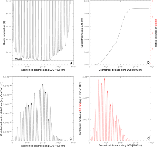
Figure 2. In panel (a), we plot the kinetic temperature along the selected LOS. In panel (b), we plot the optical thickness integrated from the left to the right along the same LOS. The y-axis on the left gives τ values at 0.45 mm and the y-axis on the right gives τ values at 9.0 mm. In panels (c) and (d), we plot, respectively, the contribution function at 0.45 mm (in black) and 9.0 mm (in red). On the x-axis in each panel, we give the geometrical distance from the first surface of the first prominence fine structure encountered along the selected LOS in units of 1000 km.
Download figure:
Standard image High-resolution imagePanel (a) of Figure 2 clearly shows that the distribution of the kinetic temperature along a typical LOS intersecting the 3D model is very structured. Steep gradients between the central minimum temperature inside individual fine structures and the maximum temperature of 100,000 K representing the PCTR in the direction perpendicular to the magnetic field are clearly visible (for more details, see Section 2). Only inside a few intersected fine structures is the central minimum temperature at the level of 7000 K—the minimum temperature set as one of the global parameters of the WPFS model (see Section 2). This may seem strange as each modeled fine structure reaches 7000 K in its central part. The reason for this is that the kinetic temperature distribution plotted here is caused by the arrangement of the fine structures within the 3D model, which is in essence stochastic. From panels (c) and (d) of Figure 2, it is clear that these contribution functions do not have globally dominant parts but have many similar local maxima distributed along the LOS.
To derive a representative value of the kinetic temperature from such complex plasma conditions, we use a concept of the weighted mean value instead of more simplified methods. As weights, we use the local values of the contribution function at 9.0 mm wavelength (panel d) of Figure 2). Such weighted-mean kinetic temperature (Tk_mean) has the largest contribution from the regions that also contribute most to the emergent intensity. This makes Tk_mean consistent with the way information about the kinetic temperature conditions is conveyed by the observed radiation. Such a dependance makes Tk_mean a good measure of the accuracy of the derived Tk_der from the observable Tb.
In the following section, we use Tk_mean to assess how well the values of Tk_der derived from the synthetic brightness temperature maps represent the real thermal conditions along the respective lines of sight in each pixel. Note that without the full knowledge of the kinetic temperature distribution—such as that provided by the 3D WPFS model—it is not possible to calculate Tk_mean.
6. Comparison Between Tk_der and Tk_mean
To assess the accuracy of the derived  , we compare it in every pixel with values of Tk_mean representing the actual kinetic temperature distribution. In Figure 3, we show scatter plots of
  with respect to Tk_mean. In panel (a), we plot all pixels from the model (over 50,000). The solid line represents
  and the dashed line shows the limit where the difference between the two is 1000 K. Panel (a) clearly shows that in a large number of pixels the difference between the derived values of
  and the actual kinetic temperature conditions along the corresponding LOS represented by Tk_mean is very large—often 5000–10,000 K. In this panel, we also highlight two selected populations of pixels. The first population contains those pixels in which the optical thickness at 9.0 mm wavelength (τ9.0) is above 0.5 (orange). The second population contains those pixels in which τ9.0 > 1 (red). These populations are also plotted separately in panels (c) and (d). Furthermore, in panels (e) and (f), we plot, respectively, only pixels where τ9.0 > 2 (blue) and τ9.0 > 3 (green). In panel (b), we overlay populations of pixels where τ9.0 > 0.5 (orange) and τ9.0 > 2 (blue). Note that while in panel (a) the x- and y-axes have a range from 0 to 80,000 K, in all other panels, the x- and y-axes range is from 7000 to 12,000 K. In panels (b) to (f), the solid line again indicates where
  . The dashed–dotted line shows the limit where the difference between
  and Tk_mean is below 500 K and the dashed line shows the limit of 1000 K.
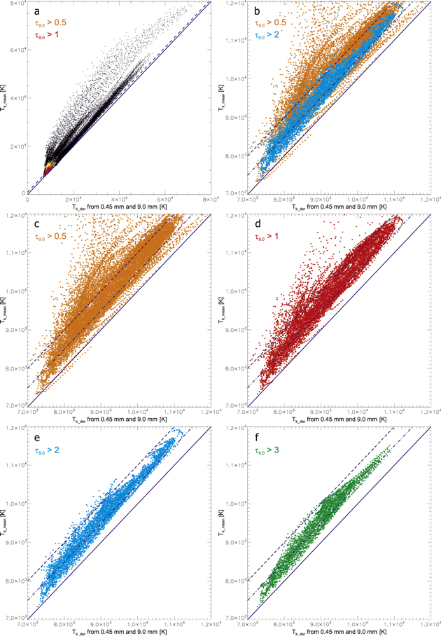
Figure 3. Scatter plots of derived values of  with respect to the weighted-mean kinetic temperature Tk_mean. In panel (a), we plot all pixels from the 3D WPFS model (black), and those where τ9.0 > 0.5 (orange) and τ9.0 > 1 (red). In panel (b), we plot only pixels where τ9.0 > 0.5 (orange) and τ9.0 > 2 (blue). In panels (c)–(f), we plot, respectively, pixels where τ9.0 > 0.5, τ9.0 > 1 (red), τ9.0 > 2 (blue), and τ9.0 > 3 (green). Solid lines represent
  , dashed–dotted lines show the limit where the difference between the two is 500 K, and dashed lines show the limit where this difference is 1000 K.
Download figure:
Standard image High-resolution imageThe discrepancy between  and the corresponding Tk_mean is greatly reduced with increasing τ9.0. However, in cases of τ9.0 > 1, and especially τ9.0 > 0.5, there are still numerous pixels where this difference is above 1000 K. Differences between
  and Tk_mean are further reduced in pixels with τ9.0 > 2 (panel e) or for τ9.0 > 3 (panel f). These differences reveal the accuracy of the method used for the derivation of Tk_der from the set of (synthetic) observations used here. For some applications, the accuracy achieved in pixels with τ9.0 > 1 may be sufficient. However, for example, for studies of energy balance in the prominence plasma, it would be beneficial to decrease possible errors below 1000 K. To achieve such an accuracy, we recommend that the limiting optical thickness at 9.0 mm wavelength is considered to be around 2.
An issue that we need to address now is whether there are enough pixels with τ9.0 > 2 to sufficiently cover the observed prominence. For our case, from panel (a) it may seem that the pixels with τ9.0 > 0.5 represent only a very small subset of all pixels. However, there are still over 17,000 pixels with τ9.0 > 0.5 and 10,000 pixels with τ9.0 > 1. This represents nearly 35% or 20% of all pixels in the used synthetic observations. For the case of τ9.0 > 2, we still have over 5000 pixels (10% of all pixels) and in the case of τ9.0 > 3 there are 3500 pixels remaining (7% of all pixels).
In this section, we have shown for which values of τ9.0 the derived  represents sufficiently well the thermal properties of the observed plasma. However, information about the actual optical thickness in individual pixels cannot be directly obtained from observations at the SMM wavelengths. Fortunately, as we show in the following section, it is possible to deduce from an observable, whether τthick is large enough to give us the confidence that Tk_der represents well the actual thermal properties of the observed plasma. This observable is
  and the deduction is based on information about the optical thickness τthick provided by the WPFS model.
7. Relationship between  and τthick

In this section, we show the relationship between the brightness temperature  at the wavelength at which the observed prominence is completely optically thin (in our case
  ), and the optical thickness τthick at the wavelength at which a significant part of the prominence is optically thick (in this case τ9.0).
In this analysis, we rely on the fact that the 3D WPFS model contains a large number of stochastically arranged fine structures and that each individual fine structure has in essence a unique plasma composition (for more details, see Section 2). This fact gives us confidence that such a complex model could produce statistically significant data sets. However, the results provided by the model can still be dependent on the choice of the global model input parameters. To take into account such a dependence, we use here two additional configurations of the 3D WPFS model. In these configurations, we vary the minimum central temperature parameter (T0) only. This input parameter can be expected to have the most significant effect on the investigation of the kinetic temperature. This is due to the fact that the choice of T0 mostly affects the distribution of the kinetic temperature of the cool plasma in the cores of the prominence fine structures. However, this cool plasma is the plasma with the highest pressure. Therefore, it contributes the most to the emergent intensity and thus to the observed Tb. In Figure 4, we show scatter plots of  with respect to τ9.0. In black, we plot results from the configuration of the 3D model used throughout the current paper (T0 = 7000 K). In blue, we plot results from a configuration where we assume that the minimum central kinetic temperature in the center of individual dips T0 is 6000 K. In red, we plot the same for a model with T0 = 8000 K. It is apparent that the distribution of the values of
  with respect to τ9.0 is rather narrow in the case of each individual configuration of the 3D model. The combined distribution for all three configurations is broader, but the overall trend is still clearly visible. In the present paper, we do not consider any other configuration of the 3D WPFS model as it can be argued that the assumed range of the parameter T0 covers the range of the most probable values of the kinetic temperature in the center of the prominence fine structures (see, e.g., Labrosse et al. 2010).

Figure 4. Scatter plot of values of the brightness temperature at 0.45 mm with respect to the optical thickness at 9.0 mm. In black, we show results of the 3D WPFS model with the minimum central temperature input parameter T0 = 7000 K, in blue are results with T0 = 6000 K and in red results with T0 = 8000 K.
Download figure:
Standard image High-resolution image
From Figure 4, it is clear that it is not possible to derive precise values of τthick from the observed  in individual pixels. However, it demonstrates that it is, in principle, possible to estimate a limiting value of
  above which τthick is in all pixels higher than the value ensuring the sufficient accuracy of Tk_der. To demonstrate this principle, we make two estimates based on the results shown in Figure 4. These are only rough estimates, which provide limiting values of
  above which all pixels in all three considered configurations of the 3D WPFS model have optical thickness above one or two. These limiting
  values are
  K for τ9.0 > 1 and
  K for τ9.0 > 2.
These rough estimates based on the results in Figure 4 serve here as a proof of concept. To better constrain the limiting values of  , we will need to perform a broader statistical analysis using a wider range of configurations of the 3D WPFS model. We will do such an analysis in the future, focusing on the wavelengths that will be used in the actual ALMA prominence observations.
8. Discussion and Conclusions
In the present work, we provide the theoretical background for the diagnostics of the thermal properties of prominences observed by ALMA. To do this, we fully exploit the potential of the 3D WPFS model of Gunár & Mackay (2015a) that provides us with the synthetic ALMA-like observations of a complex simulated prominence (see Paper I). This allows us to use the synthetic observations as if these were the actual ALMA prominence observations and to develop a technique for their analysis. The WPFS model also offers detailed information about the properties of the modeled plasma such as the distribution of the kinetic temperature and the optical thickness along any LOS. We use this unique insight to assess the accuracy of the results produced by the newly developed technique.
The ability to derive spatially well resolved information about the kinetic temperature of solar plasmas is one of the advantages of solar observations with ALMA (see, e.g., Wedemeyer et al. 2016). Such a thermal diagnostic is the goal of many current and future ALMA proposals from the solar physics community. In the present paper, we demonstrate that a measure of the kinetic temperature of the prominence plasma can be derived from a pair of SMM observations where one is obtained at a wavelength at which the observed prominence is optically completely thin and the other at a wavelength at which a significant portion is optically thick. However, as we show in Section 6, the derived kinetic temperature (Tk_der) does not necessarily represent well the actual kinetic temperature distribution. This is due to the fact that even in the case of the observation obtained at the SMM wavelength at which the observed prominence is optically thick, the actual optical thickness (τthick) may not be sufficient in every pixel. In those pixels where τthick is low, the applied method for derivation of Tk_der (see Section 3) cannot produce correct results. As we demonstrate in Section 6, the optical thickness τthick needs to be larger than unity for Tk_der to be a sufficiently accurate representation of the actual kinetic temperature distribution. For applications, such as the study of the prominence energy balance, where the accuracy of the information about the kinetic temperature needs to be high, the value of the optical thickness τthick should be larger. To keep the difference between the derived Tk_der and Tk_mean (the weighted-mean kinetic temperature representing the actual kinetic temperature distribution) reliably below 1000 K, the optical thickness τthick should be above 2.
The major problem lies in the fact that from SMM observations alone it is not possible to distinguish if the derived Tk_der in a given pixel correctly describes the actual thermal properties. We show here that this problem can be solved by taking into account the information about the optical thickness in every pixel provided by the 3D WPFS model. As we show in Section 7, it is possible to find a minimum value of the brightness temperature  above which the optical thickness τthick is with a great confidence higher than a certain value. To demonstrate this fact, we provide a rough estimate of the minimum value of
  above which τ9.0 is larger than 1 or 2. These estimates are
  K for τ9.0 > 1 and
  K for τ9.0 > 2. These numbers are valid for the pair of SMM wavelengths assumed here and are based on a limited statistical analysis. A broader statistical study is needed to constrain the limiting values of
  more adequately. We will perform such a study in the future, assuming a wider range of input parameters of the 3D WPFS model. This future study will be focused on the SMM wavelengths that will be used for the actual ALMA prominence observations. It is important to note here, that while it is in principle possible to estimate with a reasonable accuracy limiting values of
  above which the optical thickness τthick is higher than a certain value, it is not possible to derive precise values of τthick from the observed
  in each pixel.
In the present paper, we use synthetic prominence observations at the SMM wavelengths from ALMA bands 9 and 1. None of these bands is available at the time of writing of the present paper for solar observations. However, results presented here show that to achieve the highest relevance of the information about the kinetic temperature of prominence plasma derived from SMM observations, we need to use a pair of wavelengths where, at one, the observed prominence is completely optically thin and, at the other, its significant part is optically thick. To ensure that this will be true in most cases of ALMA prominence observations, the widest possible range of ALMA wavelengths should be utilized. Therefore, our present work serves also as an argument for the further development of the ALMA capabilities available for solar observations.
In conclusion, we note that our present study shows that in the case of prominences composed of numerous fine structures, a typical LOS will intersect a large number of them. Therefore, the contribution function obtained along such an LOS will have a number of often comparable local maxima but not a global maximum (see panels c and d of Figure 2). The derived Tk_der thus does not correspond to any local value of the kinetic temperature but represents an averaged value such as Tk_mean. This means that the thermal structure of prominences cannot be analyzed by deriving the local kinetic temperature values at different depths by varying the used SMM wavelength–a technique usually called the temperature tomography (see, e.g., Loukitcheva et al. 2015).
S.G. and P.H. acknowledge the support from grant 16-17586S of the Czech Science Foundation (GAČR). S.G. and P.H. acknowledge the support from project RVO:67985815 of the Astronomical Institute of the Czech Academy of Sciences. S.G. and P.H. thank for the support from the MPA Garching. U.A. thanks for the support from the Astronomical Institute of the Czech Academy of Sciences. D.H.M. acknowledges financial support from the STFC, the Leverhulme Trust, and NASA. ALMA is an international partnership of the European Southern Observatory (ESO) representing its member states, the U.S. National Science Foundation (NSF) and the National Institutes of Natural Sciences (NINS) of Japan, together with NRC (Canada), NSC and ASIAA (Taiwan), and KASI (Republic of Korea), in cooperation with the Republic of Chile. The Joint ALMA Observatory is operated by ESO, AUI/NRAO, and NAOJ. S.G. is an expert member of the Solar Simulations for the Atacama Large Millimeter Observatory (SSALMON) network.