


Abstract
Plasma parameters such as the electron density and temperature play a key role in the dynamics of the solar atmosphere. These characteristics are important in solar physics because they can help us to understand the physics of the solar corona, the ultimate goal being the reconstruction of the electron density and temperature distributions in the solar corona. The relations between emission and plasma parameters in different timescales are studied. We present a physics-based model to reconstruct the density, temperature, and emission in the EUV band. This model, called COronal DEnsity and Temperature (CODET), is composed of a flux transport model, an extrapolation model, an emission model, and an optimization algorithm. The CODET model parameters were constrained by comparing the model's output to the TIMED/SEE record instead of direct observations because it covers a longer time interval than the direct solar observations currently available. The most important results of the current work are the recovery of SSI variability in specific wavelengths in the EUV band, as well as the variations in density and temperature during large timescales through the solar atmosphere with the CODET model. The evolution of the electron density and temperature profiles through the solar corona in different layers during solar cycles 23 and 24 will be presented. The emission maps were obtained and they are in accordance with the observations. Additionally, the density and temperature maps are related to the variations of the magnetic field in different layers through the solar atmosphere.
Export citation and abstract BibTeX RIS
1. Introduction
The solar magnetic field and its relationship with the plasma parameters are important to consider when describing some phenomena in the solar atmosphere. The magnetic field is created in the solar interior by solar dynamo action (Dikpati & Gilman 2009). This manifestation is observed as a variety of phenomena in the solar atmosphere (Hargreaves 1995; Low 1996; Solanki et al. 2006; Mackay & Yeates 2012).
There are some processes where coronal electrons are accelerated and emit radiation, such as the acceleration by the electromagnetic field of photospheric radiation (i.e., EUV emission is produced by free–free emission from the chromosphere and corona). In general, the Solar Spectral Irradiance (SSI) influences the Earth's atmosphere for each wavelength in different altitudes. The EUV emission has a considerable impact on the Earth's upper atmosphere, i.e., on the density, temperature, and total electron content, and it is an important driver for space weather (Haberreiter et al. 2014; Schmidtke 2015).
The study of plasma parameters such as electron density and temperature can contribute to understanding some phenomena shown in the solar atmosphere. Determinations of coronal densities have been made since ∼1950 from the models of van de Hulst (1950) and Pottasch (1963, 1964) based on eclipse observations and empirical laws relating brightness with height. However, the measurement of these parameters is not trivial in the solar corona because the plasma is optically thin, and the information received is integrated along the line of sight, mixing information from different wavelengths (Singh et al. 2002; Kramar et al. 2014). For this reason, it is important to build models that can be used to study this behavior and check whether or not the results are related to characteristics of the solar cycle and if they are changing in different timescales.
Density and temperature profile variation along the solar cycle is an important factor and provides clues for solar corona dynamics. On the other hand, the problem of the heating corona is of great interest for solar physics. The primary conclusion is that the heating can be explained by processes that involve magnetic fields (Galsgaard & Nordlund 1997). In this context, we decided to build a physics-based model that relies on the assumption that the density, temperature, and emission variations are due to the evolution of the structure of the solar magnetic field. The COronal DEnsity and Temperature (CODET) model allows us to investigate some important aspects such as variations of density and temperature through the solar corona, in different heights and timescales. These variations are examined in large scale during solar cycles 23 and 24. This model is based on the idea presented by C. Marqué and M. Kretzschmar in the poster entitled, "Forward modeling of the electron density and temperature distribution in the corona using EUV and radio observations," in the LWS meeting, Boulder, 2007.
We structure the paper as follows. In Section 2, we describe the physics-based model, the CODET model. In Section 3, the main results are presented: reconstructions of SSI variability at 19.3 and 21.1 nm, the density and temperature profiles during solar cycles 23 and 24, the density and temperature maps through different layers in the solar atmosphere, and the emission maps in different layers at 19.3 and 21.1 nm. In Section 4, the discussion is presented. Finally, concluding remarks are made in Section 5.
2. The CODET Model
The CODET model (Figure 1) uses a flux transport model of Schrijver (2001). The flux transport model is a key component of the proposed model. The flux transport model employed line-of-sight magnetic field data from SOHO/MDI and SDO/HMI full-disk magnetograms. These data are assimilated into the flux transport model to describe the dynamics of the solar photosphere. In this approach, we could not directly employ the magnetic field strength density from MDI/SOHO (Scherrer et al. 1995) and HMI/SDO (Scherrer et al. 2012). The main reason is that the synoptic maps do not correctly take into account the evolution of the active regions as they transit in the far-side. Additionally, most of the time, synoptic maps do not cover the evolution of poles.
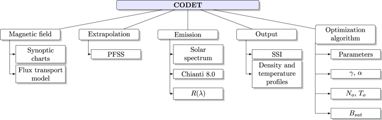
Figure 1. Schematic description of the COronal DEnsity and Temperature (CODET) model.
Download figure:
Standard image High-resolution imageThe evolving surface-flux assimilation model is sampled every six hours from 1996 July 1. The assimilation model assumes that the magnetic field from SOHO/MDI and SDO/HMI is strictly vertical and the magnetograms are incorporated within 60◦ from disk center. The assimilation procedure is a straightforward mapping: after re-binning to a resolution of 8 arcsec, each magnetogram pixel is assumed to correspond to a single concentration at the corresponding latitude and longitude. In addition to the assimilated magnetograms, small magnetic bipoles ( Mx) are injected outside the assimilation area. This maintains the quiet-Sun network, which impacts the flux dispersal even though it adds little to the large-scale coronal field. Also, bipoles are inserted on the far-side of the Sun depending on the pattern and magnitude of the measured travel time differences of p-modes reflecting around the antipode of disk center (Schrijver & De Rosa 2003).
These data are then used as boundary conditions for a series of potential-field source-surface (PFSS) extrapolations.3
The structure of the coronal magnetic field is estimated employing the PFSS model (Schrijver 2001; Schrijver & De Rosa 2003). The PFSS extrapolates the line-of-sight surface magnetic field through the corona, with the boundary assumed to be at the source surface and assuming that the solar corona is current-free. The magnetic field is extrapolated from the photosphere at  to the corona at
  .
.
The flux transport model is from the scheme of Schrijver (2001). This model considered fickian diffusion in all scales. The flux injection is described by a combination of random processes, capturing the properties of flux evolution (the flux emergence from the interior, flux dispersal over the surface, and the flux disappearance from the photosphere). After the flux in a bipolar region has fully emerged, the region decays and the flux disperses across the surface. The flux dispersal in the photosphere is frequently modeled as a passive random walk diffusion, involving supergranulation, meridional flow, and differential rotation. The bipolar region source function is

where ![$A[\mathrm{Mx}]$](https://content.cld.iop.org/journals/0004-637X/852/2/137/revision1/apjaa9f1cieqn4.gif) is the flux injection parameter related to different levels of activity, and
is the flux injection parameter related to different levels of activity, and ![$S[{\deg }^{2}\approx 150\,{\mathrm{Mm}}^{2}]$](https://content.cld.iop.org/journals/0004-637X/852/2/137/revision1/apjaa9f1cieqn5.gif) is the area of the bipolar regions. At solar cycle maxima, the coefficients
is the area of the bipolar regions. At solar cycle maxima, the coefficients  and p = 1.9 are determined by a fit to the area distribution for emerging active regions as derived by Zwaan & Harvey (1994), a1 is the set to
  in order to match the total flux input. The weaker cycle dependence for the ephemeral region frequency compared to the active region frequency is approximated through a power-law scaling with the flux emergence parameter A with a power-law index
  (Schrijver 2001).
Also, we use an emission model. This model is based on the CHIANTI atomic database 8.0 (Del Zanna et al. 2015) using specific lines (19.3 and 21.1 nm) in the EUV band. This model considers the coronal abundances and ionization equilibrium to build the solar spectrum and modeling the electron density and temperature through the solar corona.
Additionally, an optimization algorithm was used. The optimization algorithm Pikaia is a method for optimization based on a genetic algorithm (Charbonneau 1995). The Pikaia algorithm was used to determine some parameters in different problems such as the study of solar phenomena. It was used for empirical modeling of the solar corona (Gibson & Charbonneau 1998), Doppler shifts of solar ultraviolet emission lines (Peter & Judge 1999), and modeling the evolution of the solar irradiance (Krivova et al. 2007, 2010; Vieira & Solanki 2010; Vieira et al. 2011). In this case, the Pikaia algorithm was used to search the best-fit parameters of the CODET model.
2.1. Approach
The density and temperature profiles are related to the magnetic field. It is considered the thin flux tube model (Solanki 1993); the magnetic field is bundled into discrete elements of concentrated flux, called frequently magnetic flux tubes. These tubes cover fractions of the solar surface (Fligge & Solanki 2000). The flux tubes are narrow, the inflow of radiation through the hot walls exceeds the energy blocked. The geometry of the small-scale fields causes a non-isotropic radiation field. The combination of these effects leads to variations in the solar irradiance on timescales from days, to years (Vieira et al. 2012).
A pressure balance is considered between the tube and the ambient (Vekstein & Katsukawa 2000).
The vertical flux tubes are assumed not to be curved and thus do not have magnetic tension (neglecting the second term of the Equation (2)). Then, the pressure balance requirement is

where ![$N[{\mathrm{cm}}^{-3}]$](https://content.cld.iop.org/journals/0004-637X/852/2/137/revision1/apjaa9f1cieqn9.gif) is the electron density,
is the electron density, ![${k}_{B}[\mathrm{erg}\,{{\rm{K}}}^{-1}]$](https://content.cld.iop.org/journals/0004-637X/852/2/137/revision1/apjaa9f1cieqn10.gif) is the Boltzmann constant,
is the Boltzmann constant, ![$T[{\rm{K}}]$](https://content.cld.iop.org/journals/0004-637X/852/2/137/revision1/apjaa9f1cieqn11.gif) is the temperature, and
is the temperature, and ![$B[{\rm{G}}]$](https://content.cld.iop.org/journals/0004-637X/852/2/137/revision1/apjaa9f1cieqn12.gif) is the magnetic field. Also, the plasma β (
is the magnetic field. Also, the plasma β ( ) from the Equation (3), is assumed to be small enough for the plasma to be effectively confined by the magnetic field (Emslie & Brown 1980).
Then, considering the magnetic field:
where  ,
,  , and
, and  are the magnetic field components from PFSS. The magnetic field B is measured in
 ![$[{\rm{G}}]$](https://content.cld.iop.org/journals/0004-637X/852/2/137/revision1/apjaa9f1cieqn17.gif) units. We consider
units. We consider  in the following description.
In this approach, we use scaling laws for coronal loops in hydrostatic energy balance (Rosner–Tucker–Vaiana (RTV) scaling law). Scaling laws provide important diagnostics and predictions for specific physical models of the solar corona. These models have been widely applied in plasma physics, astrophysics, geophysics, and biological science (Aschwanden et al. 2008). Scaling laws can be derived both from observations and theory, and the results can be described some characteristics and phenomena in the solar corona. We follow the simplest rule, the dependence on the squared electron density, which is also proportional to the optically thin emission measure (EM) in EUV, and thus to the observed flux (Aschwanden 2005). In general, the RTV scaling laws express an energy balance, using approximations of constant pressure (Equation (3)), no gravity and uniform heating. A special case of scaling law is related to magnetic scaling.
Here we employ the density and temperature distribution in function of the magnetic field. This dependency is employed by several authors, for example: Robbrecht et al. (2010); Vekstein & Katsukawa (2000); Yokoyama & Shibata (2001); Golub et al. (1980); Golub (1983); Emslie (1985); Brown et al. (1979). We use scaling laws to describe the density and temperature profiles in function of the magnetic field. These models also take into account other parameters such as the flux tube loop length (L), volume (V), and heat conditions (τ). Mandrini et al. (2000) discuss in detail the scaling laws employed by different models of coronal heating and their relation to the magnetic field. In our model, we decided to consider the dependency solely on the magnetic field intensity; that is, the model exponents for the loop length (L) and volume (V) are considered equal to zero. The main reason for this assumption is related to the number of free parameters needed in the optimization algorithm and the time needed to parameterize each flux tube. Also, it is assumed that the total plasma pressure remains unchanged in each flux tube (Equation (3)). Then, an analytic treatment is possible, thus highlighting the essential physics of the simplified problem and allowing us to develop the simple scaling laws (Emslie 1985). We employ the distribution of density and temperature in the following way:

We consider the function Bf (R)

where ![${b}_{f0}[{\rm{G}}]$](https://content.cld.iop.org/journals/0004-637X/852/2/137/revision1/apjaa9f1cieqn19.gif) units and
units and ![$\tau {b}_{f}[{R}_{\odot }]$](https://content.cld.iop.org/journals/0004-637X/852/2/137/revision1/apjaa9f1cieqn20.gif) units are constant values (in this case, we use
units are constant values (in this case, we use  and
and  ); R corresponds to the height through the solar atmosphere, and it varies from
  to
to  . It was defined to describe two different temperature regimes related to regions with strong or weak photospheric magnetic field, using the following conditions:
- if

- If


where γ and α are power-law indices,  is the factor related to the amount of flux in each pixel,
 ![${B}_{s}[{\rm{G}}]$](https://content.cld.iop.org/journals/0004-637X/852/2/137/revision1/apjaa9f1cieqn28.gif) is a constant value of the magnetic field, and
is a constant value of the magnetic field, and ![${N}_{o}[{\mathrm{cm}}^{-3}]$](https://content.cld.iop.org/journals/0004-637X/852/2/137/revision1/apjaa9f1cieqn29.gif) and
and ![${T}_{o}[{\rm{K}}]$](https://content.cld.iop.org/journals/0004-637X/852/2/137/revision1/apjaa9f1cieqn30.gif) are background density and temperature, respectively. The temperature T and electron density N are measured in units of
are background density and temperature, respectively. The temperature T and electron density N are measured in units of ![$[{\rm{K}}]$](https://content.cld.iop.org/journals/0004-637X/852/2/137/revision1/apjaa9f1cieqn31.gif) and
and ![$[{\mathrm{cm}}^{-3}]$](https://content.cld.iop.org/journals/0004-637X/852/2/137/revision1/apjaa9f1cieqn32.gif) , respectively. Additionally, this approach evaluated the exponent value of the scaling law in B. In addition, temperature considerations between open and closed field lines are defined in Equations (7) and (8).
, respectively. Additionally, this approach evaluated the exponent value of the scaling law in B. In addition, temperature considerations between open and closed field lines are defined in Equations (7) and (8).
2.2. Emission Measure Formalism
Different models were employed to describe the emission measurement in different wavelengths (Vernazza et al. 1981; Warren et al. 1998; Kretzschmar et al. 2006; Warren 2006). In this section, some characteristics of EM formalism used in the CODET model will be described.
Assuming that the emission lines are optically thin, it is possible to measure only the integrated emission along a given line of sight, but it is necessary to consider the ionization and recombination coefficients related to the contribution function. This emission line depends on the atomic transitions and the conditions of the solar atmosphere. The specific intensity can be described by:

where ![$G(\lambda ,T)[\mathrm{erg}\,{\mathrm{cm}}^{3}\,{{\rm{s}}}^{-1}\,{\mathrm{sr}}^{-1}]$](https://content.cld.iop.org/journals/0004-637X/852/2/137/revision1/apjaa9f1cieqn33.gif) is the contribution function from the CHIANTI atomic database 8.0,
is the contribution function from the CHIANTI atomic database 8.0, ![$d\lambda [\mathrm{nm}]$](https://content.cld.iop.org/journals/0004-637X/852/2/137/revision1/apjaa9f1cieqn34.gif) is the differential element in wavelength, N
is the differential element in wavelength, N ![$[{\mathrm{cm}}^{-3}]$](https://content.cld.iop.org/journals/0004-637X/852/2/137/revision1/apjaa9f1cieqn35.gif) is the electron density, ds [cm] is the differential distance along the line of sight, and
is the electron density, ds [cm] is the differential distance along the line of sight, and  is the instrumental response.
The contribution function was used to construct the solar spectra for a specific wavelength. This function contains relevant atomic physical parameters such as ionization equilibrium and coronal abundances. The ionization equilibrium from Mazzotta et al. (1998) and coronal abundances from Meyer (1985) were used. These models consider the solar corona as optically thin. Some of these contribution functions are shown in Rodríguez Gómez (2017) and Rodríguez Gómez et al. (2017); whereas the instrumental response depends on wavelength and temperature, it constitutes an important specification of the instruments. In this case, we consider  (ideal case).
The intensity I is the full-disk average intensity measured at Earth from an emission line, where  .
.

2.3. Optimization Algorithm
The optimization algorithm was used to search the best-fit parameters of the CODET model. In order to implement Pikaia Algorithm, we use BELUGA, which is a MATLAB optimization package and is freely available from Medical School at University of Michigan in the virtual physiological Rat Project.4 BELUGA finds a local minimum x of an objective function within an initial population of candidate solutions. The free parameters are defined as follows:

where par is the free parameter that will be optimized by Pikaia algorithm, parmax and parmin are the lower and upper limits of parameters, respectively, par(n) should be located at the interval [0, 1], and n is the number of free parameters. A goodness-of-fit  is calculated between TIMED/SEE and modeled data; in general
  indicates an acceptable fit. The goodness-of-fit is the key point between the Pikaia algorithm and the model of plasma parameters (Figure 2).
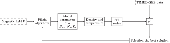
Figure 2. Schematic description of optimization algorithm Pikaia, where dashed boxes describe the input parameters.
Download figure:
Standard image High-resolution imageThe optimization algorithm was applied to fit two wavelengths 19.3 and 21.1 nm. The model parameters γ, α, Bs, No, and To were adjusted. Several cases were explored to search the best fit between TIMED/SEE data and data from the CODET model. The  function was defined after several tests as
where Imodel is the intensity from our model and Iobs corresponds to the intensity of TIMED/SEE data. In this case, a period of ten days was chosen during solar cycles 23 and 24 (2003 February 01, 2003 October 01, 2004 October 01, 2005 October 01, 2007 October 01, 2008 October 01, 2009 October 01, 2011 October 01, 2014 October 01, 2016 October 01 at 12:00 UT). The characteristics evaluated in each case were
- (1)goodness-of-fit between SSI from TIMED/SEE and modeled data; and
- (2)
The SSI data used in this work is the TIMED/SEE from the NASA TIMED mission's Solar EUV Experiment (SEE) EUV Grating Spectrograph (EGS) merged with a model driven by The SORCE XUV Photometer System (XPS). The Model uses GOES XRS measurement data and CHIANTI spectral models as well. The CHIANTI spectral model includes the differential emission measures (DEMs) and also isothermal spectra appropriate for the Sun. It has been developed to process the measurements from broadband photometers. They are combined to match the signals from the XPS and produce spectra from 0.1 to 40 nm in 0.1 nm intervals (Woods et al. 2008, 2005; Woods & Rottman 2005). Table 1 lists the parameters employed in Equations (5) and (8) that are used to compute the SSI (Equation (10)). In general, the parameter values correspond to  ,
,  and
and  .
.
Table 1. CODET Model Parameters: γ, α, No, To, and Bs
| Parameter | Value | Units |
|---|---|---|
| γ | 2.4459 | ⋯ |
| α | −1.8502 | ⋯ |
| No |

|
![$[{\mathrm{cm}}^{-3}]$](https://content.cld.iop.org/journals/0004-637X/852/2/137/revision1/apjaa9f1cieqn46.gif)
|
| To |

|
![$[{\rm{K}}]$](https://content.cld.iop.org/journals/0004-637X/852/2/137/revision1/apjaa9f1cieqn48.gif)
|
| Bs | 4.4080 |
![$[{\rm{G}}]$](https://content.cld.iop.org/journals/0004-637X/852/2/137/revision1/apjaa9f1cieqn49.gif)
|

|
0.0017 | ⋯ |
| Population size | 20 | ⋯ |
| Generation | 70 | ⋯ |
Note. Typical values for best fits and specifications about the optimization algorithm:  , population size, and generation.
Download table as: ASCIITypeset image
3. Results
3.1. Solar Spectral Irradiance
SSI at Extreme UltraViolet wavelengths (EUV) drives physical and chemical processes. The EUV solar irradiance is the most important parameter to monitor space weather. The SSI variation at EUV wavelengths has important consequences for the Earth's upper atmosphere because the SSI is completely absorbed into the tenuous layers above the stratosphere (Schöll et al. 2016; Fontenla et al. 2017). Several models of EUV have been developed since the 1970s, based on the reference irradiance spectrum and its extrapolation using proxies and using the different features of the solar atmosphere (Kretzschmar et al. 2004; Ermolli et al. 2013; Thuillier et al. 2014; Schöll et al. 2016).
The emission at EUV wavelengths originates in the solar chromosphere, transition region, and corona; it is affected by the Sun's magnetic field dynamics (Warren et al. 1998; Aschwanden 2005). The SSI varies on timescales of minutes to days, the 27-day solar rotation period (manifested into synoptic charts using that input in this approach), and the 11-year solar cycle (this variation was analyzed in this article). The CODET model has, as an output, the SSI from the photospheric magnetic field evolution over solar cycles 23 and 24 (Figure 3(a)) computed for three lines simultaneously (17.1, 19.3, and 21.1 nm), but the best results were obtained in two wavelengths: 19.3 and 21.1 nm.

Figure 3. Solar Spectral Irradiance (SSI) using the CODET model (green line) and Solar Spectral Irradiance from TIMED/SEE (blue line), SDO/EVE (black line), and SDO/AIA (red line). (a) SSI at 19.3 and 21.1 nm during solar cycles 23 and 24. (b) The best-fit interval of Solar Spectral Irradiance (SSI) from the CODET model from 2010 July 01 to 2012 July 31.
Download figure:
Standard image High-resolution imageThe scatter plots were obtained in each case, and the chi-squared test ( ) was calculated. The chi-squared test was obtained for EVE/SDO (
 at 19.3 nm and
  at 21.5 nm) and AIA/SDO (
 at 19.3 nm and
  at 21.5 nm) data to review the consistency of the modeled values in comparison with observed data. The
  values from TIMED and EVE are very similar (
 at 19.3 nm and
  at 21.5 nm); this fact allowed us to declare that the model parameters adequately describe observational data and their variations in long and short timescales. Two branch trends can be noticed: one of them overestimates observations slightly while the other underestimates them. The specific interval from 2010 July 01 to 2012 July 31 was selected to highlight the variations in a short temporal scale. The variability was recovered and follows the observational data trend from EVE and AIA data sets (Figure 3(b)). However, the EVE data are lower than the CODET, TIMED, and AIA data at 21.5 nm. In general, the SSI from CODET model is consistent with daily variations from the instruments on board the SDO spacecraft. On the other hand, the correlation coefficient (R) analysis shows a strong linear relationship between modeled and TIMED data in both wavelengths (R = 0.750 at 19.3 nm and R = 0.796 at 21.5 nm). Also, the Rvalue between EVE and CODET data shows a medium-weak relationship (R = 0.518 at 19.3 nm and R = 0.523 at 21.5 nm); while the correlation coefficient shows a weak relationship between the AIA and modeled data (R = 0.332 at 19.3 nm and R = 0.332 at 21.5 nm).
3.2. Density and Temperature Profiles during Solar Cycles 23 and 24
Due to the problem with the direct measurements of the plasma parameters, profiles of electron density and temperature from the CODET model (Section 2.1) will be presented in this section.
The plasma parameters—more specifically, the electron density and temperature—show an interesting behavior through the solar atmosphere. The transition region demarcates the boundary where the chromospheric temperature increases and the density drops, also through the solar corona the temperature increases (from  to
to  ) while the density decreases (from
  to
to  ). These trends were reconstructed using the CODET model (Figure 4).
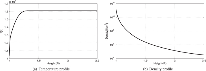
Figure 4. Temperature profile (left panel) and density profile (right panel) through the solar atmosphere on 2001 December 15; specifically from  to
to  , for the parameter combinations shown in Table 1.
Download figure:
Standard image High-resolution imageThe evolution of the electron density and temperature profiles were obtained using Equations (5) and (8) and the parameters of the model were shown in Table 1. The electron density and temperature average profiles were obtained from different layers through the solar atmosphere R = 1.14, 1.19, 1.23, 1.28, 1.34, 1.40, 1.46, 1.53, 1.61, 1.74, 1.79, 1.84, and 1.90 R⊙. Variations in temperature and density during the last solar cycles are displayed in Figure 5.

Figure 5. Average temperature (upper panel) and density (lower panel) profiles from CODET model, through different layers: R = 1.14, 1.19, 1.23, 1.28, 1.34, 1.40, 1.46, 1.53, 1.61, 1.74, 1.79, 1.84, and 1.90 R⊙, during solar cycles 23 and 24.
Download figure:
Standard image High-resolution imageLower values in temperature are shown in solar cycle 23, while in solar cycle 24, the temperature increases. The density values are higher in solar cycle 23 and lower in solar cycle 24. The external layers show lower values in average density than the layers near the photosphere.
3.3. Density and Temperature Maps
Density and temperature maps in two different layers (R = 1.16 and 1.30 R⊙) in the solar atmosphere are shown in Figure 6. The magnitude of the magnetic field was obtained from PFSS model from Equation (4) in these specific layers. For these purposes, three days were selected: 2001 December 15, 2003 November 15, and 2015 February 05.
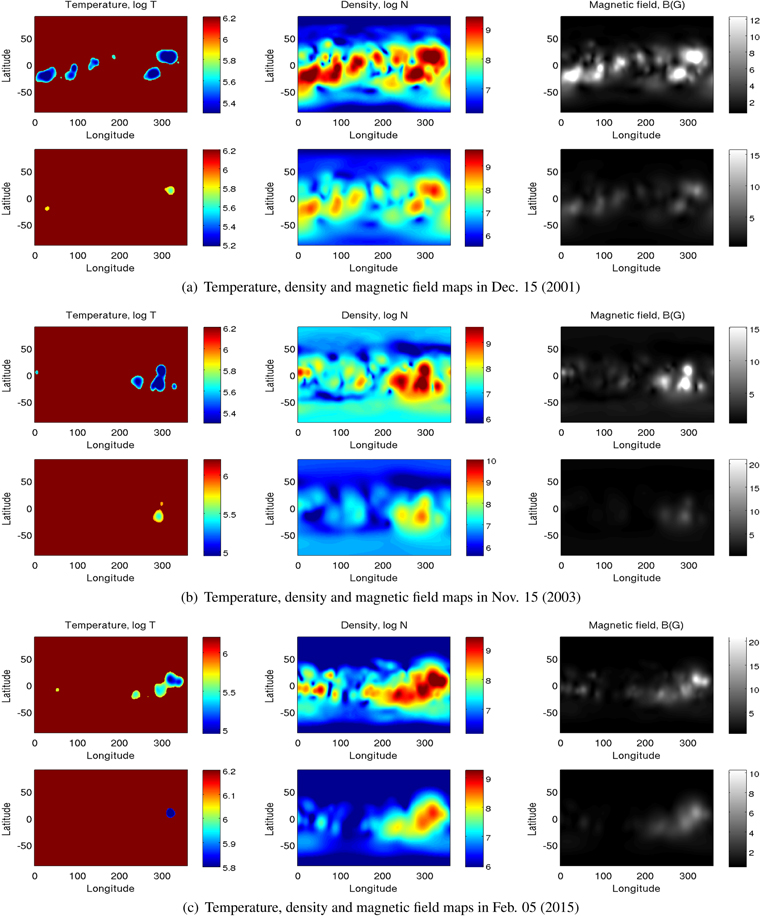
Figure 6. Comparison between temperature, density, and magnitude of magnetic field in different layers first row  and second row
  , using the CODET model. First column: temperature maps (log T); second column: density maps (log N; last column: magnetic field maps (B(G)), (a) 2001 December 15, (b) 2003 November 15, and (c) 2015 February 05. All plots show different scales to highlight the characteristics in each day and layer.
Download figure:
Standard image High-resolution imageFigure 6 shows regions with higher values in density in regions with a stronger magnetic field. These regions are related to ARs located in the active region belts. The temperature maps show some structures with medium and lower values when the magnetic field is more intense. The temperature maps show the temperature variations from  to
to  , while the density maps show variations from
  to
to  .
.
3.4. Emission Maps
The emission maps were obtained using two wavelengths, 19.3 and 21.1 nm, in three different layers of the solar atmosphere R = 1.33, 1.42, and 1.60 R⊙, on specific days: 2001 December 15, 2003 November 15, and 2015 February 05.
Figures 7 and 8 show the intensity maps in the transition region and the solar corona. The emission maps show regions with higher values in intensity over the Active Regions (ARs) and lower values in emission in areas where the filaments between ARs and the non-polar coronal holes are located, shown as dark regions close—or inside—the activity belts. The ARs display the typical appearance, similar to those of EUV observations, exhibiting more brightness than the quiet Sun. The emission maps in both wavelengths are correlated to the observational data: in 2001 December 15 and 2003 November 15 with EIT/SOHO; in 2015 February 05 with AIA/SDO.
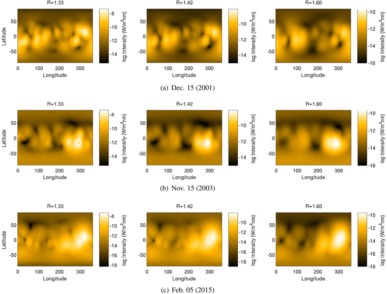
Figure 7. Intensity maps at 19.3 nm in three different layers: R = 1.28, 1.43, and 1.60 R⊙. These plots show the different scales in each layer.
Download figure:
Standard image High-resolution image4. Discussion
The CODET model is not dependent on the filling factors and the areas of the photospheric features, which form a frequent description of the semi-empirical models of the SSI (Krivova et al. 2007; Vieira & Solanki 2010; Vieira et al. 2011; Ermolli et al. 2013; Ball et al. 2014; Yeo et al. 2014). Additionally, the CODET model can describe the evolution of temperature and density in the solar atmosphere using the photospheric magnetic field.
On the other hand, we cannot directly employ the filtergrams from SOHO and HMI instruments in the optimization process, because the computational resources needed are far beyond the computational capability that we have available now. In this way, we decided to present disk-integrated values that could be directly compared to SSI observations to constrain the model. It is important to highlight that our model provides a description of density and temperature through the solar corona based on observations of the solar surface potential magnetic field. As far as we know, it is the first attempt to describe the density and temperature for two solar cycles. We point out that our model, as all models, is an incomplete description of the physical phenomena investigated. Even the most sophisticated MHD models are employed to describe just some features observed of the evolution of the density and temperature of the solar corona for a very limited timescale.
The CODET model employs a general view of the evolution of the magnetic field in the photosphere, expressed in solar synoptic maps. Also, the  factor is dependent on the spatial resolution of the instruments (Chapman et al. 2011); in our case, we use data from MDI and HMI. This can contribute to differences between modeled and observational SSI. Also, another reason for these discrepancies relates to changes during the solar rotation, because of the possibility of unaccounted instrumental drifts (Marchenko et al. 2016). However, using these data sets, it is possible to reconstruct SSI and TSI (Yeo et al. 2014).
Some observational uncertainties can influence the SSI variability, because the uncertainties may differ in units and dimensions from one data set to another (Schöll et al. 2016). Besides, the variation in a short timescale was recovered during solar cycles 23 and 24 (Figures 3(c) and (d)), which corresponds to the results presented in Marchenko et al. (2016) for short periods of cycles 23 and 24.
We point out that due to the lack of suitable observations in the EUV spectral region for the period of that we employed to constraint the model, the model parameters were constrained by comparing the models' output to the TIMED/SEE record, which employs model reconstructions to fill data gaps.
The temperature and density profiles are strongly dependent on the magnitude of the magnetic field, and two power-law exponents describe these variations, α for the temperature and γ for the density profile (Section 2.1). In this description, γ has positive values while α has non-positive values in all tests described in Rodríguez Gómez (2017). These power-law exponents were found independently through the optimization algorithm Pikaia, and it retrieves parameters that describe properly the SSI variations during the last solar cycles. This relationship between power-law exponents generates the temperature profiles that are inversely proportional to the magnetic field, while the density profile is directly proportional to the magnetic field (Figure 5). Other less successful parameter combinations were explored for 17.1, 19.3, 21.1, and 33.5 nm in Rodríguez Gómez (2017).
The temperature profiles show a slight increase in the solar cycle 24 compared with the solar cycle 23. In the external layers, the temperature is higher than in the internal layers during the two last solar cycles. The solar cycle 23 shows lower temperature values than the solar cycle 24 due to the modeled temperature profile was described as inversely proportional to the magnetic field (Equation (8), Table 1, and Figure 5, upper panel). Thus, the variations in temperature through the solar atmosphere are highly variable, and this behavior is shown in temperature profiles from CODET model due to the dependence between temperature and emission in the EUV band.
The density profiles show lower values in the external layers and higher values in layers near the photosphere. Higher values in the density profiles are more common during solar cycle 23 as compared to solar cycle 24. The electron density profiles follow the sunspot trend during the solar cycle, and they are related to the variations of the magnetic field, because the density profile is proportional to the magnetic field (Equation (5), Table 1, and Figure 5, lower panel).
Besides that, the temperature and density profiles in Figure 4 are in accordance with the single-fluid radiative energy balance model through the inner corona presented in Withbroe (1988). That approach employs some empirical values based on measurements of the intensity, polarization of the electron-scattered white light corona, and measurements of the radial intensity gradients of EUV spectral lines to constraints on temperature in the solar corona. In this model, the source of the radiated energy is mechanical energy transported and dissipated in the corona by undetermined mechanisms.
The temperature maps obtained from the CODET model (Figure 6) show small regions with values in an interval from  to
to  in the two selected layers. These values were reported in the empirical temperature maps in the EUV wavelengths: 21.1, 19.3, and 17.1 nm (Dudok de Wit et al. 2013). Likewise, our results are in agreement with temperatures related to EM analysis and with the observations (Winebarger et al. 2011; Aschwanden et al. 2013).
The density maps from the CODET model are quite well correlated with the magnetic field strength. Tripathi et al. (2008) found that the density in an AR is  and references therein suggests values of
  . The CODET model shows maximum values of
  , which is agreement with values reported in the literature. These behaviors are shown in Figure 6 and they are in agreement with the work of Kramar et al. (2014). Additionally, we have focused on the active region belts (Abramenko et al. 2010) and their structures as ARs and non-polar CHs.
The emission description (Equation (9)) is related to the optically thin emission. In our approach, using the definition of DEM in the same way (Warren et al. 1998; Aschwanden 2005; Hannah & Kontar 2012), the density and temperature profiles are defined a priori from Equations (5) and (8). Also, we include the contribution function and the atomic data from the CHIANTI atomic database 8.0 for EUV lines, in the same way was presented at Fontenla et al. (2014).
The emission maps were explored in three layers: R = 1.33, 1.42, and 1.60 R⊙ and two wavelengths 19.3 and 21.1 nm. Regions with higher values in emission are related to regions with higher values in density, which are the ARs (Figures 6–8). We mainly focus on ARs and CHs inside a belt of  around the solar equator because the PFSS do not describe regions located in latitudes
  adequately (Abramenko et al. 2010); therefore, it is not reliable for modeling polar CHs. This is corroborated by visual inspection of the observed images from EIT/SOHO in 19.5 nm and AIA/SDO in 19.3 and 21.1 nm. The ARs and non-polar CHs are reconstructed adequately. Non-polar CHs and regions between ARs that may harbour filaments are also in agreement with observations. Additionally, Warren et al. (2012) describe an inverse correlation between the EM and unsigned magnetic flux for lower (approximate, transition region) temperatures, while the EM and unsigned flux are directly related for very high temperatures. The inverse EM and unsigned magnetic flux relationship may explain the temperature maps presented in this paper. Therefore, the evidence on EUV spectral line considerations and the physics-based model can both be in accordance with the results.

Figure 8. Intensity maps at 21.1 nm in three different layers: R = 1.28, 1.43, and 1.60 R⊙. These plots show the different scales in each layer.
Download figure:
Standard image High-resolution image
5. Concluding Remarks
The performance of the CODET model is comparable to that of the observational data from TIMED/SEE. The SSI variation between solar activity maximum and minimum is properly simulated. The agreement with the data is gratifying considering that the CODET model does not have an MHD approach (Figure 3). Moreover, it is important to highlight that the CODET model adequately describes the evolution of the magnetic flux from the quiet Sun regions or, specifically, the minimum between solar cycles 23 and 24. This behavior is probably due to the input of the CODET model. They correspond to the synoptic maps and are related to the mean variations of the magnetic flux during of a period of ∼27 days. Thus, high-cadence temporal variations in the magnetic flux from the active regions are not possible in this current version.
An important feature of the present work is a description of temperature and density profiles in the solar corona during a large timescale (the last two solar cycles). Also important are the temperature, density, and emission maps in different layers through the solar atmosphere. The emission is reconstructed for ARs and non-polar CHs in a synoptic view. An interesting relationship between higher values in emission and density is shown, and it is expected to be explored in depth in a forthcoming paper.
This work is partially supported by CNPq/Brazil under grant agreements No. 140779/2015-9, No. 304209/2014-7, and No. 300596/2017-0. J.P. thanks the MINECO project AYA2016-80881-P (including AEI/FEDER funds, EU). J.M.R. would like to thank Matthieu Kretzschmar and Thierry Dudok de Wit for the helpful discussions during the Sun-Climate Symposium, 2015, in Savannah, Georgia. We thank the anonymous reviewer their comments that helped improve this paper.
Footnotes
- 3
Solarsoftware. http://www.lmsal.com/solarsoft.
- 4