


Abstract
The interaction of siphon flow with an initially linear Alfvén wave within an isolated chromospheric loop is investigated. The loop is modeled using 1.5D magnetohydrodynamics (MHD). The siphon flow undergoes a hydrodynamic (HD) shock, which allows the Alfvén instability to amplify the propagating waves as they interact with the shock and loop footpoints. The amplification leads to nonlinear processes strongly altering the loop equilibrium. Azimuthal twists of  are generated and the loop becomes globally twisted with an azimuthal magnetic field of
  . The flow is accelerated to
  due to the propagating shock waves that form. Near the end of the simulation, where the nonlinear processes are strongest, flow reversal is seen within the descending leg of the loop, generating upflows up to
  . This flow reversal leads to photospheric material being "pulled" into the loop and spreading along its entirety. Within about 2.5 hr, the density increases by a factor of about 30 its original value.
Export citation and abstract BibTeX RIS

Original content from this work may be used under the terms of the Creative Commons Attribution 3.0 licence. Any further distribution of this work must maintain attribution to the author(s) and the title of the work, journal citation and DOI.
1. Introduction
Magnetic flux tubes are ubiquitous in the solar atmosphere and they provide the structure for many interesting features to arise. In the photosphere, flux tubes are abundant within sunspot umbrae and penumbrae. In the chromosphere and corona, flux tubes are seen to form the basis of a multitude of magnetic structures such as spicules and prominences. The topology of these magnetic structures can vary widely, with tubes being near constant in radius or expanding, near vertical or highly inclined, or they may even form loops or loop-like structures.
Many of these flux tube structures often exhibit mass flow such as siphon flows in coronal loops (Orlando et al. 1995a, 1995b), counterstreaming (Lin et al. 2003) and field-aligned flows within filament channels (Lin et al. 2005), upflows in spicules (Hollweg et al. 1982; De Pontieu et al. 2004; Zaqarashvili & Erdélyi 2009; Scullion et al. 2011), and Evershed flows within sunspots (Montesinos & Thomas 1997; Plaza et al. 1997).
In the corona, numerous studies have modeled/interpreted prominences as structures embedded within twisted flux tubes (or flux ropes) (Okamoto et al. 2009; Priest et al. 1989; van Ballegooijen & Martens 1989; Wang & Stenborg 2010; Keppens & Xia 2014; Filippov et al. 2015; Yang et al. 2016, and so on). A property of a loop structure is that it may exhibit a siphon flow. These siphon flows have long been studied in the context of the solar environment and were first studied in magnetic flux tubes in relation to the Evershed effect in sunspots (Meyer & Schmidt 1968). Subsequent studies have since investigated these siphon flows within magnetic flux tubes (Cargill & Priest 1980; Thomas 1988; Orlando et al. 1995a, 1995b; Montesinos & Thomas 1997; Grappin et al. 2005; Taroyan 2009; Bethge et al. 2012, and others). Wang & Stenborg (2010) observe transverse motions of  within a prominence cavity where the spin direction aligns with the strongest to weakest magnetic field of the footpoints across the polarity inversion line (PIL). They interpret this asymmetry as a siphon flow before the cavity and adjacent streamer loops become "pinched" to form a flux rope. Orlando et al. (1995a) developed a model of equilibrium conditions for siphon flows within coronal loops using and comparing two independent numerical codes. Orlando et al. (1995b) built upon this by studying stationary (adiabatic and isothermal) shocks within coronal loops for supersonic and critical siphon flows. Tsiropoula (2000) found flows of 5–15 km s−1 within sunspot penumbral fibrils, which are reminiscent of siphon flows.
Yang et al. (2003) observed the penumbra formation of a sunspot in an active region NOAA 9539. They found that the formation of penumbral filaments near the light bridge separating two pores indicated the sudden change of magnetic topology from near-vertical field lines to strongly inclined ones. This allowed material that was previously suspended in the filament to flow downwards. During this downflow, Hα Dopplergrams revealed twisted streamlines along the filament. Similar timescales of 20–30 minutes have been observed by Leka & Skumanich (1998), Schlichenmaier et al. (2010) for penumbral filament formation as Yang et al. (2003). Similarly, Yang et al. (2003), and Leka & Skumanich (1998) both see more inclined field lines in the penumbral areas than the umbra, and that the Evershed flow is coupled to inclined magnetic fields. Schlichenmaier et al. (2010) observe the formation of a penumbra on a leading spot without penumbra and pores (active region NOAA 11024), which takes just under 5 hours to form a sunspot in which more than half of the umbra is surrounded by penumbral filaments.
Much work has been done in the formation of dynamic fibrils and spicules (Hollweg et al. 1982; Hollweg 1992; Kudoh & Shibata 1999; James et al. 2003; Erdélyi & James 2004; Jess et al. 2009; Matsumoto & Shibata 2010). Mass flow tracing the magnetic filed lines and torsional twisting is observed in these structures, which are believed to be due to Alfvén waves. Their presence can be detected through non-thermal broadenings (Jess et al. 2009) and/or the simultaneous presence of blueshifted and redshifted Dopplergrams within a single structure (De Pontieu et al. 2014). While spicules are often modeled as near-vertical structures in magnetohydrodynamics (MHD) simulations, it has long been known that they are often inclined or curved such that they are near horizontal, such as that shown in Figure 1 of Foukal (1971).
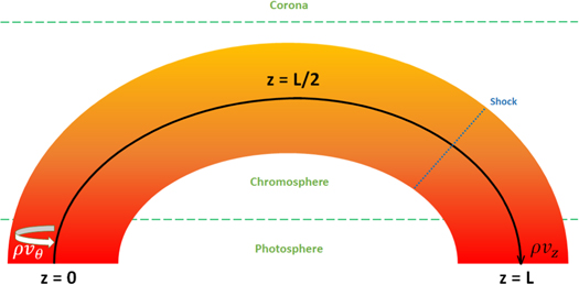
Figure 1. A schematic showing the geometry of the model employed during the study. The flow propagates from z = 0 to z = L and undergoes an HD shock in the descending leg of the loop. Both footpoints are situated in the photosphere.
Download figure:
Standard image High-resolution imageIn this paper, we present a mechanism associated with siphon flows that could play an important role in prominence, filament channel, and/or spicule formation and their dynamics. An initial loop of high inclination is assumed. The footpoints of the loop reside in/near the photosphere and a siphon flow is employed between them. Following from previous studies (Orlando et al. 1995b; Williams et al. 2016), the supersonic flow becomes subsonic as it passes through a hydrodynamic (HD) shock. A small amplitude magnetic twist is introduced to the system and it becomes amplified through the Alfvén instability discussed in previous work (Taroyan 2008, 2009, 2011, 2015; Taroyan & Williams 2016; Williams et al. 2016).
In Section 2, we discuss the model used for the study, the results of which are presented in Section 3 and discussed in Section 4 with reference to current literature. Concluding remarks are made in Section 5.
2. Numerical Method
In previous work (Williams et al. 2016), one end of the flux tube was rooted in the photosphere and the other was open ended. This allowed us to model the Evershed effect in sunspots. However, in this study we wish to study the Alfvén instability in a highly inclined loop. The high inclination means that gravity may be neglected. Another implication is that both ends of the flux tube are now rooted in the photosphere. The footpoints are treated in such a way that they are allowed to bend in response to plasma and wave motion within the flux tube.
We impose Dirichlet boundary conditions for the azimuthal momentum  at each end of the flux tube. All other boundary types (ρ,
  , e,
, e,  , and Bz) are Neumann boundary conditions where
  . The adopted line-tying boundary conditions represent magnetic field lines anchored in a dense photosphere. These types of line-tying boundary conditions are commonly adopted in studies of atmospheric dynamics (e.g., Hood & Priest 1979; Goedbloed & Halberstadt 1994; Ofman et al. 1998; Belien et al. 1999; De Groof & Goossens 2002).
In our model, the Dirichlet boundary condition is imposed by setting the ghost cells boundary type to asymmetric. This copies and multiplies the nearest two-mesh cells by −1. This ensures any perturbation interacting with the boundary changes sign upon reflection as opposed to being "squashed" and "skipping" off the photosphere. This prevents a non-physical, continual twist in one direction or the other. It can be checked that a requirement on both vθ and Bθ vanishing at the boundaries would imply either a flow speed equal to the Alfvén speed or a degenerate set of conditions on vθ and Bθ and their derivatives to vanish at the boundaries. Instead, we only require the first derivative of Bθ to vanish at the boundaries. These boundary conditions are discussed in more detail in Williams et al. (2016, Section 2.4).
A supersonic flow that is sub-Alfvénic is introduced and undergoes a shock that is located in the descending leg of the loop so as to be consistent with Orlando et al. (1995b) and to replicate what would likely occur to the flow within the loop if gravity were included in the simulations.
The numerical code used to model our loop is VAC (Versatile Advection Code; Tóth 1997). The fourth-order central differencing method (CD4) is used in combination with the minmod limiter and TVDLF (Total Variance Diminishing Lax-Friedrich) predictor step.
The model presented in this paper is a 1.5D axisymmetric magnetic tube, which was introduced by Hollweg et al. (1982) and subsequently employed by Sterling & Hollweg (1988), Kudoh & Shibata (1999), Matsumoto & Shibata (2010); and others. It is discussed by Hollweg (1981) that a single field-line is modeled that resides close to but not on the axis of symmetry, such that for typical cylindrical coordinates,  at any point. The equations used in these models may describe torsional and shear Alfvén waves in the nonlinear regime depending on whether the chosen geometry is cylindrical or Cartesian (Priest 2014, Section 4.3). A consequence of the geometry employed is that θ denotes the azimuthal direction, where it is assumed that
  .
.
The 1.5D model consists of 3000 gridpoints of uniform spacing, and the ideal-MHD equations solved are given by Hollweg (1992):


where

and

For brevity,  , and
, and  . The plasma density, longitudinal and azimuthal velocities, internal energy, as well as the longitudinal and azimuthal magnetic field components are given by: ρ, vz,
  , e, Bz, and
  , respectively.
The nonlinear coupling between the azimuthal and longitudinal variables is given by ptot in Equations (2) and (4). As is the case with Williams et al. (2016), the conservation of energy can be expressed through combining Equations (4), (6), and (7), which yields
The thermal, kinetic, and magnetic energy densities are given in the temporal derivative of Equation (8).
Equation (8) describes the evolution of the total energy. In the Appendix, we derive the following equation for the azimuthal (twist) component of energy:

The left-hand side of Equation (9) contains the time derivative of the azimuthal energy density and the spatial derivative of the azimuthal energy flux. The right-hand side (RHS) of Equation (9) contains a source term

where  is the azimuthal magnetic energy density. This source term,
  describes how kinetic energy of the flow is converted into magnetic twist and is derived in Taroyan & Williams (2016) for a linear system. In the Appendix, we have shown that the terms remain valid for this nonlinear study.
The azimuthal component of the energy flux,  in Equation (9) is defined as
Equation (9) shows that an accelerating (decelerating) flow corresponding to 
 leads to the possibility of energy transfer between the longitudinal and transverse motions even in the linear regime. This wave-flow coupling plays a key role in the amplification of small amplitude twists, the consequences of which we study here.
We use the energy Equations (8) and (9) to define the following terms:

and

Here,  ,
,  , and
, and  are the azimuthal components of total energy, kinetic energy, and magnetic energy densities. Wz is the total longitudinal energy density, where
  , and Wth represent the z-component of the kinetic energy density, and the thermal energy density of the plasma.
Integrating Equation (9) between 0 and L and rearranging yields

where  is the total azimuthal energy along the loop.
  and
and  are the azimuthal energy fluxes at the footpoints, z = 0 and z = L, respectively. The last term on the RHS of (14) describes the total contribution of wave-flow coupling,
  along the entirety of the loop.
2.1. The Loop Model
The loop is situated between the two footpoints at z = 0 and z = L, with the loop apex situated at  (Figure 1). A supersonic flow emanates from within the photosphere and propagates along the loop until it undergoes an HD shock at
  . The shock is described in terms of the Rankine–Hugoniot jump conditions


where

and

Here, the sound speed is given by cS, while subscripts 1 and 2 denote the plasma upstream and downstream of the shock.  is the sonic Mach number of the upstream plasma,
  is the adiabatic index, R is the molar gas constant, ξ is the molar mass, and T is the plasma temperature. The Alfvén speed within the loop is,
  . Using the definition of Alfvén speed,
  , and given that
  , and the normalization of B and
  is done so that
  within VAC, cA can be used to infer the magnetic field strength, B = 9. Pressure, p1 = 0.833 at the z = 0 boundary is calculated from Equation (19).
We provide some example values that can be obtained through parameterization of these variables to make the model consistent with the solar atmosphere; however, all results shown are normalized quantities. Assuming a sound speed of  within the loop yields flow and Alfvén speeds of
  and
and  , respectively. Similarly, given the Alfvén speed and taking
  , the magnetic field strength can be deduced to be,
  . Using Equation (19) and the values obtained for cS1, and
  , pressure within the loop is,
  . The length of the loop is
  with a resolution of
  . As the loop is highly inclined, the elevation remains below
  , i.e., within the chromosphere of a conventional model atmosphere. The total simulation time equates to: 2h23m24s with one unit time,
  = 33m20s.
2.2. Alfvén Wave Driver


3. Results and Analysis
A single azimuthal pulse that is determined by expression (20) is launched from the footpoint at z = 0, t = 0. The pulse propagates along the loop until it interacts with the stationary shock. The Alfvén wave is partially transmitted through the shock from the upstream plasma into the downstream plasma, with the rest of the wave being over-reflected by the shock (Acheson 1976; Williams et al. 2016) and propagating back towards the z = 0 boundary. Once the reflected pulse reaches and interacts with the z = 0 footpoint, it is reflected back up and along the flux tube for the process to repeat until the wave becomes nonlinear.
The portion of the Alfvén wave that is partially transmitted through the stationary shock propagates out of the simulated flux tube in our previous study (Williams et al. 2016). However, as we are now simulating a loop whose footpoints are embedded within the photosphere, the wave is now reflected and partially transmitted at z = L.
When the wave propagates in the  direction after reflection from the photosphere
  , it again interacts with the shock where it is both partially transmitted into the upstream plasma and reflected back towards z = L. The portion of the Alfvén wave that passes through the shock into the upstream plasma is free to merge with the Alfvén wave trapped between the shock and z = 0, and potentially accelerate the amplification process further (Supplementary Movie 1).
This amplification may be explained through Equation (14). In general, the azimuthal energy influx,  exceeds the outflux,
  as the flow speed is higher at the left footpoint. However, even if the two balance each other, the flow gradient is negative at the shock front; thus, the RHS of Equation (14) is positive. It follows that as the RHS is positive, the azimuthal energy density, Wθ, of the wave must increase regardless of the direction of propagation.
Each time the Alfvén wave in region 1 is partially transmitted through the shock into region 2, it also aids the amplification of the Alfvén wave trapped between the HD shock and z = L. This wave amplification occurs as the two Alfvén waves coalesce and merge into a single pulse. This continual feedback between the two regions either side of the shock is not possible in Williams et al. (2016) due to one end of the flux tube being open. The magnetic energy of the Alfvén wave is free to escape through the boundary in that study, but this is no longer the case with both ends now being firmly rooted into the photosphere.
The azimuthal time–distance plots (Figure 2 and 3) show that the amplification process takes until  for the Alfvénic perturbations to begin forming strong gradients. Around this time, the nonlinear coupling becomes apparent, and secondary, fast and slow-mode waves can be seen in vz (Figure 4) and ρ (Figure 5). The fast- and slow-magnetoacoustic waves propagate with phase speeds of cA, and cS in a static medium (Priest 2014). In our case, we have a flowing plasma; thus, the phase speeds are
  and
and  , where the + (−) sign denotes wave propagation with (against) the flow.

Figure 2. Time–distance plot for  is shown in a) with the associated color bar. Panels b) and c) show the magnetic twist for the entire simulation at positions
  , and
, and  , respectively.
Download figure:
Standard image High-resolution image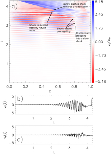
Figure 3. Time–distance plot for  is shown in a) with the associated color bar. Panels b) and c) show the azimuthal twist velocity for the entire simulation at positions
  , and
, and  , respectively.
Download figure:
Standard image High-resolution image
Figure 4. Time–distance plot for vz is shown in a) with the associated color bar. Panels b) and c) show the flow velocity for the entire simulation at positions  , and
, and  , respectively.
Download figure:
Standard image High-resolution image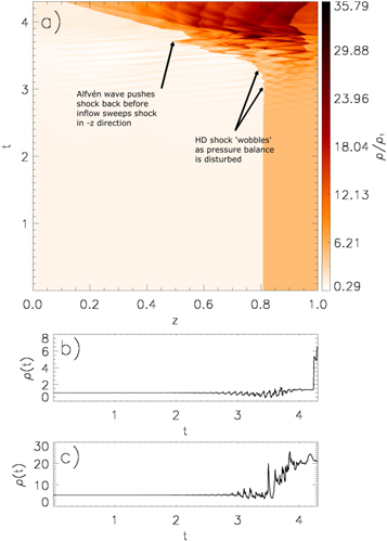
Figure 5. Time–distance plot for ρ is shown in a) with the associated color bar. Panels b) and c) show the density for the entire simulation at positions  , and
, and  , respectively.
Download figure:
Standard image High-resolution imageThe amplification of the twist velocity continues until it reaches a maximum of  . This maximum corresponds to the Alfvén wave trapped between the z = 0 footpoint and the HD shock. The associated magnetic twist,
  begins to form a global twist between
  , which can be seen in panel a) of Figure 2. The magnetic field twisting appears strongest during the period where the Alfvén waves disturb the HD shock the greatest.
Around this time, it can be seen that there is localized acceleration in the upstream plasma (Figure 4), which also leads to regions of decreased density (Figure 5). Between  , there is also localized deceleration present, which subsequently leads to localized density increases in region 1. These localized variations are the result of fast-mode waves that are coupled to the Alfvén waves, which steepen into propagating shocks as the Alfvén waves continue to amplify.
The Alfvén waves behave somewhat differently in the upstream plasma when compared with the downstream counterparts. Figure 5 shows that there is an accumulation of mass in the downstream plasma. This coincides with the Alfvén waves extracting kinetic energy sufficiently enough that the downstream plasma becomes quasi-static. Eventually, due to the nonlinear coupling in the momentum (2) and energy (4) equations, the Alfvén waves incite an inflow from the z = L boundary, which can be seen clearly in Figure 4. The decrease in the mass outflux and the subsequent influx through the z = L footpoint are responsible for the mass accumulation.
The time–distance plot for cS (Figure 6) shows us that, prior to the HD shock being disturbed and propagating to the z = 0 footpoint, there is a decrease in the sound speed of the downstream plasma before it increases rapidly. This rapid increase suggests that there is a strong increase in pressure, leading to shock heating, and an imbalance of the initial conditions (15)–(19). This increase in sound speed coincides with the flow reversal at the z = L footpoint.
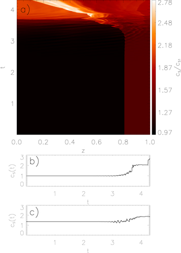
Figure 6. Time–distance plot for cS is shown in a) with the associated color bar. Panels b) and c) show the sound speed for the entire simulation at positions  , and
, and  , respectively.
Download figure:
Standard image High-resolution imageAs is discussed by Williams et al. (2016), this pressure imbalance leads to the stationary shock propagating. Between  , there is a sudden increase in the sound speed in region 1. This halts the propagation of the shock in the negative z direction, and "pushes" it back along the loop in the positive z direction. This can be seen most clearly in Figure 5 at
  ,
,  . However, this sudden change in upstream plasma pressure appears to invoke a region of larger pressure immediately downstream. This could be a consequence of the flow reversal as there are now two, oppositely propagating flows colliding into one another. This pressure increase leads to a localized region of sound speed that is comparable with the initial supersonic flow along the loop. Once again, this imbalance forces the HD shock to propagate in the negative z direction towards the z = 0 footpoint.
In addition to these variations in the thermal pressure either side of the HD shock, there is also a discontinuity that forms in vθ. This is caused by the presence of a slow shock forming at the stationary shock location (Supplementary Movie 2; Figure 3 at  ).
).
Figure 7 shows the maximum density within the loop as a function of time with the overall mass overplotted. It reveals that the Alfvén waves generate localized accumulation of mass, which precede the increase in total mass of the loop. As these localized events die down ( ), the mass continues to increase. This may be explained by the z = L footpoint becoming a region of inflow. Thus, the accumulation of mass is a result of a mass flux decrease and subsequent reversal at the z = L footpoint.

Figure 7. Maximum density (red) within the loop as a function of time is shown. The maximum can be seen to increase by a factor of 6.87. The total mass within the loop is also plotted (blue).
Download figure:
Standard image High-resolution imageThe distribution of the plasma-β (Figure 8) reveals that  initially. The presence of Alfvén waves trapped in the downstream plasma lead to an increase in β when the waves incite an inflow of photospheric material from the z = L footpoint of the chromospheric loop. Even at this point, where β reaches a maximum, it remains less than unity.
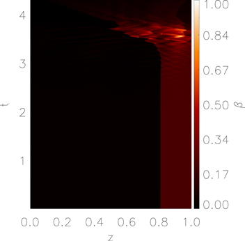
Figure 8. Spatial and temporal distribution of the plasma-β.
Download figure:
Standard image High-resolution image3.1. The Critical Evolution Period
In this subsection, we focus on the period deemed to be pivotal in the system evolution. This period is between  and
and  . This is where the nonlinear process most drastically alters the flux tube and requires a more rigorous analysis. For this, the expressions (12)–(14) are used to generate several time–distance plots (Figures 9–13).

Figure 9. Time–distance plot for the θ-energy component, given by Equation (12) in panel a). Panel b) shows the total  within the loop.
Download figure:
Standard image High-resolution imageFigure 9 shows that the total azimuthal energy increases in an exponential manner during  . The top panel shows that the propagating waves amplify upon interaction with the HD shock as well as the two footpoints at z = 0, and z = L. There is also amplification in
  when two waves propagating in opposite directions interact with each other. The azimuthal energy sees its greatest magnitudes in the downstream plasma (both immediately after the shock, and at the z = L footpoint). The propagating sound waves/shocks that form as a consequence of the Alfvén waves lead to periodic increases in Wzk in the upstream plasma as they are reflected from the z = 0 footpoint (Figure 10). Figure 10 shows that the kinetic energy term of Equation (13) amplifies greater in the upstream than the downstream plasma (until the flow reversal begins), while Figure 11 shows the opposite is true for the thermal energy.

Figure 10. a) Time–distance plot of the first term on the RHS of Equation (13), Wzk. The corresponding integral from  is shown in panel b).
Download figure:
Standard image High-resolution image
Download figure:
Standard image High-resolution imageAround  , the Alfvén waves interact with the downstream plasma, converting kinetic energy (Figure 10) into azimuthal energy (kinetic and magnetic; Figure 9) and thermal energy (Figure 11). This energy conversion can be seen as regions of brightening at
  in Figures 9 and 11. This conversion is caused by the nonlinear coupling of Equations (2) and (4). As the waves interact with the z = L boundary, the footpoint alternates between being a region of outflow and inflow. A large wave propagates through the HD shock at
  , which sufficiently disturbs the pressure balance either side of the stationary shock and causes it to move slowly towards z = 0. As the pulse is reflected at z = L, the nonlinear coupling is sufficient to turn the outflow to a strong inflow at the boundary. This reaches a maximum of
  .
.
This conversion of an outflow to an inflow leads to an increase in ρ. This is because the Alfvénic shock propagating in the downstream plasma converts the kinetic energy of the flow to magnetic energy. This conversion gradually leads to the z = L footpoint becoming a region of permanent influx, matching z = 0. In turn, this additional influx from z = L is what leads to the accumulation of mass downstream of the HD shock. The flow reversal also leads to enhanced influx of azimuthal magnetic energy through the two footpoints (Equation (9)).
If we look at the azimuthal energy flux at the two footpoints, which is given as  , it becomes clear that the net influx seen in Figures 12, and 13 arises due to the presence of the HD shock. From Supplementary Movie 2, Bθ is approximately the same at z = 0 and z = L, but vz is not. This means the difference in azimuthal energy flux, i.e., the larger influx at z = 0 than outflux at z = L, is caused by the presence of the stationary shock. If there was no classical shock, and given that gravity is not present, the flow would travel at the same speed along the entire loop. Thus, there would be no net energy flux as the total influx and outflux at the footpoints would be equivalent and therefore the azimuthal energy density would remain constant.
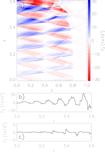
Figure 12. a) Time–distance plot for the magnetic flux,  . The flux at
  and
and  are shown in panels b) and c).
Download figure:
Standard image High-resolution imageThe azimuthal magnetic flux along the tube and the associated helicity would remain constant in the absence of a longitudinal flow. The situation is different when there is a flow gradient along the tube. Consider the induction Equation (5) and integrate it over the length of the loop, 0 to L:
Applying the limits yields:

where  denotes the total azimuthal magnetic flux. A consequence of the line-tying boundary conditions is that
  at z = 0 and z = L. Thus, the RHS is 0, and the expression can be rearranged and expanded to:

It can be seen from the time–distance plot (Figure 2) and the Supplementary Movie 2 that  increases along the entirety of the loop as the simulation develops. It follows from Equation (23) that as the LHS increases, the RHS must be positive. Again, this means the azimuthal magnetic flux increase is responsible for the continual twisting of the magnetic field. The corresponding increase in the azimuthal magnetic energy can be seen in Figure 9.
While we have seen that the footpoints are a source of amplification for the Alfvén waves and subsequently the nonlinear processes, it is important to note that the role of the HD shock is more important than merely providing the conditions for asymmetric flux to arise. If we consider the source term described by Equation (10) and its subsequent plot (Figure 13, bottom panel) then it is clear that there is amplification at the shock front too. This is because  , and from Equation (10), we see that sθ is positive when the flow gradient is negative. In our case, the only negative gradient within the modeled flux tube is at the shock front. This means
  will be large at the shock when a twist is present. As the magnetic twists become more prevalent,
  becomes significant within the loop where Alfvénic waves propagate into one another. The source term is notably a region of localized amplification, i.e., it only becomes prominent in regions of strong, negative flow gradients. If the gradient is positive, then
  would convert magnetic energy into kinetic energy.
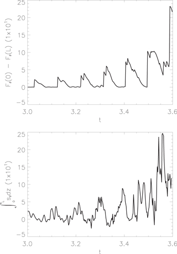
Figure 13. Top: the difference in azimuthal magnetic energy flux between the two footpoints. Bottom: the integral along the length of the loop for  is shown.
Download figure:
Standard image High-resolution image
If we compare the net energy flux caused by the asymmetry of the siphon flow between the two footpoints with sθ (Figure 13), then it becomes clear that both play a major role in the amplification of the Alfvén waves. That is, neither one or the other provide more energy to the Alfvén waves. However, it is important to remember that without the presence of the flow gradient, neither mechanism would operate.
4. Discussion
In this paper, we have demonstrated the effects of the Alfvén instability within a highly inclined loop. As with our previous study (Williams et al. 2016), the Alfvén wave gains magnetic energy from the conversion of kinetic energy of the flow and from the net influx of azimuthal energy through the footpoints. This process is somewhat reminiscent of Fermi acceleration (1st order), or diffusive shock acceleration. That is, where charged particles undergo acceleration through repeated reflection by a magnetic mirror. It is thought to be the primary mechanism by which particles gain non-thermal energies in astrophysical shock waves. In our case, the classical shock acts as a magnetic mirror, allowing constant amplification of the Alfvén waves upon reflection.
The introduction of a second Dirichlet boundary means the conditions for amplification are no longer restricted to an instability criterion (Taroyan 2008; Williams et al. 2016, for example). This allows for almost any  ratio to generate an instability leading to amplification of an Alfvén wave or wave-train.
As is common with siphon flows, our model exhibits asymmetric flux between the z = 0 and z = L footpoints. This asymmetry arises due to the difference in flow speed between the two footpoints and is a consequence of the hydrodynamic shock in the descending leg of the loop. If we consider Equation (14), it can be seen that for the azimuthal energy to increase, the RHS has to be positive. This means amplification may occur due to a net influx of azimuthal energy between the footpoints,
or through wave-flow coupling,

In the presence of negative flow gradients,  is positive—in this case, at the shock interface. This means the Alfvén wave extracts kinetic energy from the flow and converts it to magnetic energy as it interacts with the shock. The energy provided by the net influx at the footpoints and wave-flow coupling at the shock interface are approximately equal. As such, it is impossible to say one source is more important than the other during the amplification process.
The nonlinear coupling between the θ-components and z-components in Equations (3) and (4) allows the formation of propagating waves, both fast- and slow-mode. These steepen into shock waves as the Alfvén waves amplify further. This leads to localized alterations of the flow speed, reaching speeds of  .
.
A consequence of the nonlinear Alfvén waves is the conversion of the footpoint at z = L from an outflow to a source of inflow. This upflow reaches similar velocities,  as those observed by Berger et al. (2008). Subsequently, this new source of inflow "pulls" photospheric plasma through the footpoint into the loop. This leads to the mass accumulation seen where
  . This influx, along with the Alfvén waves, alters the magnetic and thermal pressures to the point where the classical shock propagates towards the z = 0 footpoint. The initial upstream plasma (z = 0 to
  ) sees a density increase of
  as the downstream plasma spreads along the loop due to the shock propagation.
During the simulation, it can be seen that a twist velocity that exceeds  and reaches a maximum greater than
  is obtained within the simulated loop. This leads to
  , meaning that the magnetic field strength within the loop increases from
  to
to  . However, in a multi-dimensional study, the twist is unlikely to reach these levels of amplification, as it is likely some form of eruption would occur—possibly due to the loop becoming kink unstable such as in Török & Kliem (2005). Reducing the Alfvén speed would allow for a weaker initial B-field, meaning the induced magnetic twist would also be smaller, and more similar to that seen in prominences.
5. Conclusion
Using our 1.5D MHD model of an isolated, highly inclined loop, we have shown that the Alfvén instability may amplify Alfvén waves in the presence of a supersonic flow. The Alfvén waves amplify upon reflection at the footpoints due to the asymmetric flux caused by the siphon flow. The Alfvén waves also amplify upon interaction and reflection with the stationary shock due to the wave-flow coupling. It is shown that the asymmetric flux through the footpoints and wave-flow coupling at the shock provide the Alfvén waves with comparable energy for amplification.
The nonlinear coupling of Equations (2) and (4) becomes prominent as the Alfvén waves continue to bounce and amplify between the shock and footpoints. The coupling leads to secondary fast- and slow-mode waves being generated within the loop. These lead to increased flow speeds of up to  .
.
The twist velocities within the simulated loop reach up to  and continually twist the magnetic field in the same direction. The azimuthal velocity incited by these waves is coherent with Type-II spicules (De Pontieu et al. 2014). Similarly, the nature of the rotation/swirls produced by our model mimic that of prominence tornadoes (Li et al. 2012). The result of this continual twist is a global magnetic twist where
  , which increases the field strength from
  to
to  .
.
As these magnetic twists reach the z = L footpoint, they convert the region from a source of outflow to inflow. This conversion of flow direction leads to upflows of  , matching observational upflows seen in prominences (Berger et al. 2008) and Type-I spicules (Beckers 1972). Subsequently, the Alfvén waves/plasma flow "pull" photospheric material into the loop, leading to mass accumulation. The density increases by a factor of 30 as a result of the nonlinear coupling. The examined novel mechanism for the formation of a twisted flux tube with enhanced density may play an important role in the formation of many structures within the solar atmosphere. However, multi-dimensional studies with the inclusion of gravity, combined with observations are required for conclusive evidence.
T.W. would like to thank the STFC for their financial support.
Appendix: Derivation of the Energy Equation
The chain rule can be applied to the θ-momentum Equation (3) so that it becomes

We multiply the θ-components of the momentum (24) and induction (5) equations by vθ and  , correspondingly

and

By taking the sum of the above two equations we obtain the time derivative of the θ-component of the energy density, Wθ
From the continuity Equation (1) we have

Substituting Equation (28) into (27) and rearranging the terms, we obtain the equation of azimuthal energy

or

where  is the azimuthal component of the energy flux.