


Abstract
We present quantitative predictions of the structure of reconnection exhausts in three-dimensional magnetic reconnection with an X-line of finite extent in the out-of-plane direction. Sasunov et al. showed that they have a tilted ribbon-like shape bounded by rotational discontinuities and tangential discontinuities. We show analytically and numerically that this prediction is largely correct. When there is an out-of-plane (guide) magnetic field, the presence of the upstream field that does not reconnect acts as a boundary condition in the normal direction, which forces the normal magnetic field to be zero outside the exhaust. This condition constrains the normal magnetic field inside the exhaust to be small. Thus, rather than the ribbon tilting in the inflow direction, the exhaust remains collimated in the normal direction and is forced to expand nearly completely in the out-of-plane direction. This exhaust structure is in stark contrast to the two-dimensional picture of reconnection, where reconnected flux expands in the normal direction. We present analytical predictions for the structure of the exhausts in terms of upstream conditions. The predictions are confirmed using three-dimensional resistive-magnetohydrodynamic simulations with a finite-length X-line achieved using a localized (anomalous) resistivity. Implications to reconnection in the solar wind are discussed. In particular, the results can be used to estimate a lower bound for the extent of the X-line in the out-of-plane direction solely using single-spacecraft data taken downstream in the exhausts.
Export citation and abstract BibTeX RIS
1. Introduction
Magnetic reconnection facilitates the conversion of magnetic energy to thermal and directed motion in many settings of importance to solar, heliospheric, and astrophysical plasmas (Zweibel & Yamada 2009). The classical models of Parker (1958) and Petschek (1964) were considered in two dimensions (2D), invariant in the out-of-plane direction, for simplicity. There are numerous examples where information learned in 2D theory and simulations has been profitably used to interpret satellite observations and laboratory experiments (e.g., Mozer et al. 2002; Ren et al. 2005; Phan et al. 2007; Burch et al. 2016). However, there are also circumstances where 2D models of reconnection are insufficient (e.g., Pontin 2011 and references therein).
In this study, we investigate 3D reconnection for which the X-line is localized, i.e., has a finite extent, in the out-of-plane direction. In 2D models, the extent of the reconnecting current sheet in the out-of-plane direction is effectively infinite, or at least larger than any relevant length scale in the system. However, in any naturally occurring reconnection, the reconnecting current sheet must be of finite extent. In principle, finite-extent X-lines can either remain localized or spread (or elongate) in the out-of-plane direction.
The spreading of localized reconnection has been inferred in satellite observations, measured directly in the laboratory, and studied theoretically and numerically. Spreading of reconnection X-lines occurs, or is thought to occur, at Earth's dayside magnetopause (Phan et al. 2000; Fuselier et al. 2002) and magnetotail (McPherron et al. 1973; Nagai 1982), solar flares (as evidenced by elongating ribbons; Isobe et al. 2002; Tripathi et al. 2006; Qiu 2009; Qiu et al. 2010, 2017), and in laboratory experiments (Katz et al. 2010; Egedal et al. 2011; Dorfman 2012). In the solar wind, magnetic reconnection exhausts measuring  (Phan et al. 2006) and
  (Gosling 2007) in extent have been observed, where RE is the radius of Earth; it was suggested these exhausts are associated with extended X-lines that begin with a small extent and spread in time.
Theoretical efforts have revealed that X-line elongation in antiparallel reconnection is governed by the species carrying the current at the associated speed of the current carriers (Huba & Rudakov 2002, 2003; Shay et al. 2003; Karimabadi et al. 2004; Lapenta et al. 2006; Schreier et al. 2010; Lukin & Linton 2011; Nakamura et al. 2012; Jain et al. 2013). For reconnection with a large out-of-plane (guide) magnetic field, reconnection spreads bidirectionally at the Alfvén speed based on the guide field; for intermediate guide field strengths, the spreading occurs by whichever of the two mechanisms is faster (Shepherd & Cassak 2012).
The extent of the reconnection X-line can also remain localized. In the zero guide field case, wider current sheets exhibited X-lines with a steady length of around 10 ion inertial lengths (Shay et al. 2003). This X-line length has been shown to be the minimum stable length because the ends of the X-lines act as energy sinks (Meyer 2013).
Less attention has been paid to the properties of reconnection with an X-line of finite extent in the out-of-plane direction that does not spread. Linton & Longcope (2006) studied the time evolution of post-reconnection flux tubes in non-steady (bursty) reconnection analytically and compared the results with 3D resistive-magnetohydrodynamic (MHD) simulations. Sasunov et al. (2012) addressed the structure of steady (continuous) localized reconnection exhausts as part of a study into whether the Kelvin–Helmholtz instability occurs at exhaust boundaries in the solar wind. Their results are summarized in the next section; they argue for evidence of crossings of exhausts in the solar wind with only tangential discontinuities (TDs) and contact discontinuities (CDs) instead of the usually expected rotational discontinuities (RD; Gosling et al. 2005; Phan et al. 2006). A number of observed solar wind reconnection events were compared to the predicted discontinuity structure of steady localized reconnection (Sasunov et al. 2015).
The observational signatures of localized reconnection takes on particular importance for the case of extended reconnection in the solar wind. Satellites in the solar wind almost always detect reconnection at their exhausts rather than their X-line. Thus, it is a challenge to infer information about X-lines in the solar wind. In particular, it is not known whether extended exhausts in the solar wind are associated with extended X-lines (Phan et al. 2006; Gosling 2007) or whether the extended exhausts are associated with a finite-extent X-line (Sasunov et al. 2015), so there is an unresolved ambiguity. Therefore, it is useful to understand whether exhaust signatures can be used to infer properties about the extent of the X-line.
It has also been suggested that reconnection with an X-line of finite extent may play a role in the creation of supra-arcade downflows (SADs), also known as "tadpoles." SADs are dark plasma voids that appear at the top of coronal arcades. These features descend toward the Sun during solar flares (McKenzie & Hudson 1999; McKenzie 2000). It was suggested that reconnection that is localized in space is important for the creation of SADs (Linton & Longcope 2006; Cassak et al. 2013). Localized reconnection may also occur in Earth's magnetotail (Angelopoulos et al. 1997; Nakamura et al. 2004; Hietala et al. 2017).
In this study, we build on previous work by Linton & Longcope (2006) and Sasunov et al. (2012) to develop quantitative predictions of the downstream structure of exhausts of magnetic reconnection with an X-line of finite extent within the MHD approximation. It is relatively clear that for reconnection with no out-of-plane (guide) magnetic field, the exhausts are bounded by the typical slow shocks in the normal direction (within the fluid model), which is the same direction as the reconnection inflow. The boundaries in the out-of-plane direction where reconnected magnetic field lines abut magnetic field lines that do not participate in reconnection are TDs, so the finite-extent X-line is described essentially by the typical two-dimensional picture with TDs forming the boundaries in the out-of-plane direction. The absence of a guide field is a singular case, though, so the more general case is when a guide field is present. In this case, there are significant differences to the structure of the exhausts relative to the two-dimensional picture. The upstream guide field that does not reconnect acts as a boundary condition in the normal direction, which constrains the normal magnetic field to be small outside the exhaust. As a result, the normal magnetic field in the exhaust remains small. Consequently, when there is a guide field, the exhaust remains collimated in the normal direction and instead expands in the out-of-plane direction. Plasma crosses into the exhaust from the out-of-plane direction, which is completely different than the two-dimensional case. Our results are largely consistent with the qualitative result by Sasunov et al. (2012), who argued that there are potentially extended TDs even for X-lines of finite extent. Our results differ from their result, however, in that they predicted that the tangential discontinuties forming the upstream boundary of the exhaust rotate in the inflow direction when there is a guide field and the plasma inflow comes in from the upstream direction, but we argue that the exhaust does not rotate and that the inflow into the exhaust is almost fully in the out-of-plane direction. We confirm these predictions with 3D resistive-MHD numerical simulations, and discuss applications to solar wind reconnection. In particular, we show that a lower bound on the extent of the X-line can be obtained purely from single-satellite measurements at a reconnection exhaust.
This paper is organized as follows. Theoretical predictions of the structure of reconnection with a finite-extent X-line are presented in Section 2. In Section 3 the setup for simulations to test the predictions is discussed. The results of the simulations are presented in Section 4. Applications are discussed in Section 5. A discussion of the results is given in Section 6.
2. Theory
Here, we develop quantitative predictions of the physical characteristics of exhausts during reconnection with an X-line of finite extent. To do so, we employ the following simplifying assumptions. We consider a quasi-2D system, meaning that the equilibrium parameters do not depend strongly on the direction normal to the reconnection plane. We also assume that the plasma parameters are symmetric on either side of the current layer; asymmetries are not considered here.
We employ a coordinate system where x is the outflow direction, y is the normal direction (typically associated with inflow in two-dimensional reconnection), and z is out of the reconnection plane. These coordinates correspond to the boundary normal coordinates  , and
, and  , respectively. Therefore, the typical 2D reconnection plane is the xy plane, with the X-line at the origin. The X-line has a finite extent
  in the z direction. The asymptotic reconnecting and guide field strengths are Bx and Bg, respectively.
A sketch of the asymptotic magnetic field lines looking up the y-axis is given in Figure 1(a). The orange solid lines and purple dashed lines are magnetic field lines on the  and
and  sides of the reconnection region with
  and
and  , respectively. (Both have the guide field Bz = Bg in the positive z direction.) The black line indicates the X-line of finite extent. What this means is that only magnetic field lines crossing the finite-extent X-line undergo reconnection; field lines crossing z = 0 farther than
  away from the X-line do not reconnect. We depict the region where magnetic flux undergoes reconnection as the orange and purple shaded regions. After the field lines reconnect, they retreat from the X-line in the
  and
and  directions. This results in a ribbon of reconnected magnetic flux, as identified by Sasunov et al. (2012).

Figure 1. (a) Sketch of the magnetic geometry of guide field reconnection with an X-line of finite extent looking up the y-axis toward positive y. Orange (solid) and purple (dashed) lines represent magnetic fields on the  and
and  sides of the reconnection site, respectively. Reconnection only occurs between magnetic fields in the shaded regions, forming ribbon-like reconnection exhausts. (b) An oblique view of the reconnection exhaust on the
  side of the X-line. A cut in the yz plane across the exhaust forms a parallelogram (shaded gray) that becomes larger in z but remains collimated in y as it propagates farther from the X-line. The edges of the exhaust shaded red are rotational discontinuities (RDs), and the edges of the exhaust with normal in the
  direction are tangential discontinuities (TDs) in blue. See Sasunov et al. (2012) for a related sketch.
Download figure:
Standard image High-resolution imageSasunov et al. (2012) argued that the inflow edges of the exhaust are RDs. Physically, these are locations where inflow along the reconnected ribbon of flux is redirected into the exhaust. They also argued that the edges connecting the RDs are TDs. Physically, these arise at the boundary of reconnected magnetic field lines where they abut magnetic fields that do not reconnect because the X-line is of finite extent. (Their study also addressed CDs within the exhaust, but we do not address that here. There is evidence that non-MHD physics remains important even at long distances from the X-line in the exhaust (Mistry et al. 2016).) The discontinuities bounding the exhaust are sketched in Figure 1(b), showing an oblique view of a portion of the exhaust in a region downstream of the X-line toward  . The gray planes are slices of the exhaust at fixed values of x, normal to the outflow
  . Magnetic field lines in the
  and
and  domains are again drawn as orange and purple, respectively; they have undergone reconnection and are retracting in the
  direction. The blue lines denote that the reconnected magnetic field lines are essentially in the z direction in the exhaust, as we discuss further below. The RDs are shaded a translucent red and mark where plasma and magnetic fields are redirected into the exhaust. The TD at the bottom (the
  side) is shaded blue; there is another TD at the top that has been omitted for clarity. The gray planes consequently take on a parallelogram-like shape, which was pointed out by Sasunov et al. (2012).
In the study by Sasunov et al. (2012), parallelogram-shaped exhausts are tilted in the yz plane. Here, however, we argue that except for very weak guide field strengths, any tilting is weak, i.e., the exhaust remains collimated in the y direction. Consider a cut at a fixed x, which is shown in Figure 2(a). This is essentially a view up the exhaust (in the direction of  ) of the exhaust region in Figure 1(b), normal to the gray parallelogram. The magnetic field in the white regions outside the exhaust at positive and negative y does not undergo reconnection, so the boundaries are discontinuities. Tilting the exhaust in the y direction would introduce a By in the region that has not undergone reconnection everywhere outside the shaded exhaust region. This is energetically unfavorable for all but the weakest guide fields, so it would not actually happen. Therefore, the TDs bounding the exhaust have a normal essentially in the y direction. To satisfy the boundary conditions at the edge of the exhaust, By within the exhaust is also small. This is in stark contrast to two-dimensional reconnection, where By is a signature that reconnection has occurred. Here, rather than rotating into the y direction, the reconnected magnetic field rotates in the z direction. The plasma at the RD has a vy and vz, drawn with black arrows in the figure, and is redirected at the RD into the exhaust. Some features of this plot are consistent with a superposed epoch analysis of reconnection exhausts in the solar wind (Mistry et al. 2017).
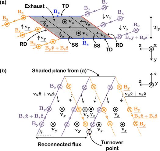
Figure 2. (a) Sketch of the exhaust and magnetic geometry in a cut normal to the exhaust (in the yz plane) at a negative value of x. The gray shaded region is the exhaust and the orange and purple fields lines are as in Figure 1. The boundaries of the exhaust are TDs in the y direction and RDs in the other two. The velocity components show the inflow redirected into the exhaust and turned into outflow. Slow shocks (SSs) are labeled as the dashed black lines. (b) Top view of the same exhaust looking up toward positive y, showing the flow. In the z = 0 plane, the exhaust is collimated following the point where the two ribbons pass through the plane. We call this the turnover point.
Download figure:
Standard image High-resolution imageWe now derive quantitative features of the exhaust structure. Figure 2(b) shows the magnetic fields and flows in the exhaust in a view looking up the y-axis toward positive y. This plot is essentially a rotation of the view from panel (a) where the bottom of the figure is made to rotate 90° into the page. The shaded plane in (a) corresponds to the black line at the top of panel (b). Flows and fields in this region are plotted using the same conventions as in panel (a). The the reconnected magnetic fields extend into the out-of-plane direction z when there is a non-zero guide field; the amount to which it does is defined by the opening angle θ measured from the z-axis, shown in the lower left corner of the figure. From the diagram, this angle is given by the relative strengths of the reconnecting and guide fields:

We now consider what the exhaust from reconnection with an X-line of finite extent looks like in the reconnection plane, specifically, the xy plane at z = 0. A sketch of the projection of magnetic fields in this plane is shown in Figure 3. The magnetic field lines in the plane open out at an angle α, corresponding to the RDs where the system has undergone reconnection. However, farther out from the X-line than the RDs, the field lines bounding the exhaust have not undergone reconnection, therefore the boundaries are TDs. Thus, in the reconnection planes at z = 0, it appears as if the RD changes to a TD; however, this is merely a geometrical effect from the way the plane intersects the ribbon bounded by RDs and TDs. We refer to the distance downstream (in x) from the X-line where collimation begins as the "turnover point," and have also labeled it at the bottom of Figure 2(b).

Figure 3. Sketch showing the projection of the magnetic field in the reconnection xy plane at z = 0. The magnetic field opens up in the inflow direction with an angle α, where  .
.
Download figure:
Standard image High-resolution imageWe can predict the downstream distance lx of the turnover point using the magnetic field geometry. As is shown in Figure 2(b), the reconnected magnetic fields (or RDs) cross at the midpoint of the extent of the X-line, indicated as the black circle. Note that θ also defines the angle between the distance to the turnover point lx and the half-extent of the X-line lz, so that  . Using Equation (1), we find the distance to the turnover point in terms of the extent of the X-line and the upstream magnetic fields to be

We can also use a geometric argument to predict the thickness ly of the collimated reconnection exhaust at the turnover point and beyond. Figure 3 shows a projection of the magnetic field to the z = 0 plane. The angle α is related both to the magnetic fields By and Bx and the distances ly and lx. Using this geometry, we find that  , so
, so  . Using Equation (2) to eliminate lx gives

The reconnected field By can be obtained by direct measurement, or it is often assumed to be 0.1 of the reconnecting magnetic field Bx (Shay et al. 1999). We will see that these predictions are useful for interpreting satellite observations of solar wind reconnection.
We point out that Equation (3) is related to a previous prediction of ly based on conservation of magnetic flux within the reconnected flux rope (Cassak et al. 2013). Cassak and collaborators found

which is the same, except that the total magnitude of  is in the denominator instead of only the guide field Bg. This difference arises because Equation (4) takes into account that the reconnected flux tube is at an angle through the xy plane, while Equation (3) is evaluated at the edges of the reconnected flux that lies at the upstream edges.
3. Simulation Setup
To test the predictions, 3D simulations are performed using the two-fluid code F3D (Shay et al. 2004). The code updates the continuity, momentum, and induction equations, and we use the resistive-MHD Ohm's law with a specified resistivity. (The plasma is assumed isothermal for simplicity, although the results are not expected to be sensitive to this choice.) The Hall term and electron inertia terms are not included for these simulations unless otherwise noted. Magnetic fields, densities, and length scales are normalized to arbitrary values  and L0. Velocities are normalized to the Alfvén speed
  . Times are normalized to
  , electric fields to
  , temperatures to
  , and resistivities to
  . As before, x is the direction of the oppositely directed field, y corresponds to the inflow direction if the simulations were 2D, and z is the out-of-plane direction.
The initial magnetic field configuration is a double tearing-mode setup where
where  is the initial half-thickness of the current sheet in the y direction. We use a constant and uniform temperature T = 1.0. Total pressure is balanced with a non-uniform density. Simulations are performed with and without a uniform guide field Bg.
Reconnection is initiated with a localized (anomalous) resistivity  , which achieves fast reconnection and allows us to fix the X-line extent in the out-of-plane direction since the X-line does not elongate in MHD. We use a resistivity of the form

where  and w0z sets the half-extent of the X-line length in the out-of-plane direction, so once reconnection commences, we have
  .
.
Simulations are performed in a 3D domain of size  . Boundaries in all three directions are periodic, but the system is long enough in the z direction that the boundaries do not affect the dynamics on the timescales of the present study. The grid scale is
  . A stretched grid in the out-of-plane direction has been used before (Shay et al. 2003; Shepherd & Cassak 2012) and is acceptable since the in-plane dynamics are on faster timescales than the out-of-plane dynamics. All equations employ a fourth-order diffusion with coefficient
  in the x and y directions. In the out-of-plane direction, the fourth-order diffusion coefficient D4z depends on the speeds in the out-of-plane direction. For
  , the fourth-order diffusion coefficient is
  for Bg = 3.0, it is
  . The values of D4z have been tested by varying the value by a factor of two to ensure that D4z does not play a significant role in the dynamics.
4. Results
We first show differences in the exhaust structure of reconnection that begins localized but spreads in the out-of-plane direction, and reconnection with an X-line of finite extent that does not spread. The former is obtained from a simulation with the same parameters as the localized resistivity simulation, but using the Hall-MHD model (including the Hall term and electron inertia) with a uniform resistivity. Both simulations have  . Figure 4 displays the reconnection exhaust vix in the xz plane in a cut through the X-line after some time has passed in a strong guide field simulation,
  . The white and black colors represent flow with a positive and negative vix, respectively. The Hall-MHD result is shown in panel (a); the rectangular shape of the exhaust occurs because the reconnection X-line spreads bidirectionally in the out-of-plane direction (Shepherd & Cassak 2012). For magnetic reconnection with an X-line of finite extent, panel (b) reveals that the reconnecting portion of the X-line remains localized to
  . The reconnection exhaust in this plane expands into the z direction forming a cone-like shape, consistent with expectations from the ribbon structure shown in Figure 2(b). An important item of note is that an exhaust of any length could be created with or without spreading because of the presence of a guide field. In other words, the presence of an extended exhaust does not imply that the X-line must also be extended, as was pointed out by Sasunov et al. (2015).

Figure 4. (a) Exhaust velocity vix at y = 0 during Hall reconnection with a guide field Bg = 3 that spreads in the out-of-plane direction. (b) Similar plot using a localized resistivity that does not spread.
Download figure:
Standard image High-resolution imageThe conical structure of the reconnection exhaust in the plane through the X-line is set by the magnetic field geometry, as predicted by Equation (1). Images of the reconnection exhaust vix for simulations with differing guide field Bg are shown in Figure 5. It is clear that the reconnection exhaust extends more in the out-of-plane direction with larger guide field. We measure the opening angle by finding the boundary of the exhaust beyond the initial reconnection region  . The boundary is chosen by taking cuts of the exhaust vix in the outflow direction, and the edge is chosen to be where
  . The measured angle is defined as
  , where Lzb and Lxb are the lengths of the boundary in the out-of-plane direction and outflow direction, respectively. The measured opening angle θ is shown as a function of guide field Bg for each simulation in Figure 6 as the triangles; the predicted angle is given as the solid line. The measured angle agrees very well with the predicted opening angle given by Equation (1).
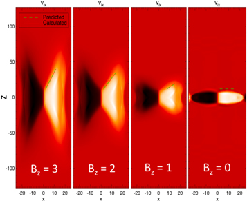
Figure 5. Reconnection exhaust velocity vix in the y = 0 plane as in Figure 4 for reconnection with a localized resistivity and guide fields of  , and 0.
Download figure:
Standard image High-resolution image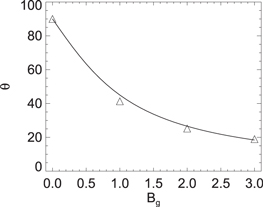
Figure 6. Exhaust opening angle θ as a function of guide field Bg. The measured angle is marked by the triangles. The predicted opening angle  is marked by the solid line.
Download figure:
Standard image High-resolution imageIn the plane of reconnection (the xy plane), the reconnection exhaust becomes collimated in the y direction. We show this in simulations with varying guide field in Figure 7, where each image is of a reconnection exhaust vix in the z = 0 plane. The normal y and outflow x directions are the horizontal and vertical axes, respectively. Each of these simulations employ the same X-line extent  . For reference, vertical dashed lines at a distance 0.5 from the center of the exhaust are included. For
  and 1.0, the exhaust expands in y and then collimates (runs parallel to the x direction) at the turnover point located at
  and 10, respectively. According to Equation (2), the turnover points are
  and 10 for
  and 1.0, respectively, in good agreement with the simulation results. As the guide field decreases, the turnover point moves farther away from the X-line. For
  , the predicted turnover point from Equation (2) is not within the simulation domain, so we see no collimation. We expect that the exhaust would be collimated farther downstream if the simulation domain was made larger. We also include a 2D simulation with
  in the panel on the right. As expected, we do not see any collimation of the exhaust, confirming that the collimation is indeed a 3D effect.
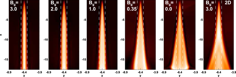
Figure 7. Reconnection exhausts in the reconnection (z = 0) plane for simulations of 3D localized reconnection with different guide fields Bg as given in each plot. The exhaust is more collimated in this plane for stronger guide fields. The rightmost plot is a 2D simulation with Bg = 3, showing what it looks like when the X-line is not localized.
Download figure:
Standard image High-resolution imageIn 2D reconnection, one often associates the opening angle with the rate of reconnection, so one might think from Figure 7 that the reconnection slows for increasing guide field Bg. However, this is not the case. In Figure 8, the reconnection rate E is shown as a function of time t for each simulation from Figure 7. We see here that the collimation of the exhaust does not affect the steady-state reconnection rate. Therefore, while in 2D a collimated exhaust implies slow reconnection, the reconnection rate is still the fast rate of order 0.1 even with a thin exhaust in 3D. This is because the total exhaust area increases with distance downstream as a consequence of the spreading in z. This is in contrast to the spreading in y in the 2D case.
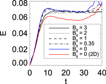
Figure 8. Reconnection rates for the simulations in Figure 7 for localized reconnection with varying guide fields and fixed X-line length w0z. The exhaust collimation in the reconnection plane does not affect the reconnection rate.
Download figure:
Standard image High-resolution imageThe X-line extent w0z in the previous simulations was fixed at 10. If we vary w0z and hold Bg constant, then according to Equation (2), the turnover point will change accordingly. This is the case in the simulations. We performed simulations with  , and 10 and found that the distance at which the exhausts become collimated is larger for larger
  these are shown in Figure 4 of Cassak et al. (2013).
We now investigate the structure of discontinuities bounding the exhausts during reconnection with an X-line of finite extent. Figure 9 shows (a) the y-component of the ion velocity viy and (b) the out-of-plane current density Jz, both in the z = 0 plane for the  simulation with
  . Flow in the
  direction is present along the exhaust in the x direction until the turnover point near x = 3. Beyond this, there is no viy and the current sheet is collimated. Since flow across a discontinuity is associated with RDs, the region until x = 3 is an RD and is associated with the ribbon of flux undergoing reconnection at the localized X-line, as sketched in Figure 2(a). Beyond the turnover point, there is no inflow so the exhaust is bounded by TDs on both upstream boundaries. Thus, in the plane of reconnection at the midpoint of the finite-extent X-line, the RD appears to extend until it reaches the turnover point and then transforms into a TD. However, as discussed in Section 2, this is a geometric effect rather than a transformation; the RD extends farther out in planes at other values of z.
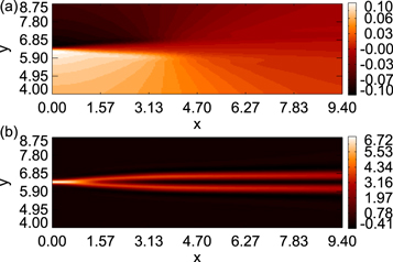
Figure 9. (a) Speed viy in the y direction in the reconnection (z = 0) plane for the  simulation. The vertical flow terminates at the turnover point of the exhaust at
  . (b) Out-of-plane current density Jz, also showing collimation of the exhaust. The turnover point is where Jz stops expanding in the y direction and becomes parallel to the x-axis.
Download figure:
Standard image High-resolution imageThis can be seen by investigating the structure of the exhausts in the yz plane, similar to the plane sketched by Sasunov et al. (2012). Figure 10 shows (a) viy and (b) the reconnection outflow speed vix for the  simulation with
  . The yz cut is taken outside the region where the exhaust collimates in the z = 0 plane. Two regions of vertical flow are located around
  and +28, but not at z = 0. This happens because the RDs propagate along reconnected field lines and leave the z = 0 plane. The top and bottom of the exhaust are TDs because there is no inflow across these boundaries. The parallelogram shape of the exhaust, as predicted by Sasunov et al. (2012), is clearly visible. However, this figure also shows that the parallelogram is not tilted into the y direction; the edges of the exhaust are nearly at a fixed y value. This is consistent with the sketch in Figure 2(a) and the discussion in Section 2.

Figure 10. (a) Speed viy in the y direction in the yz plane through the exhaust for the  simulation. The non-zero flow indicates the presence of an RD. (b) Reconnection exhaust vix in the same plane, showing the parallelogram structure from Figure 2.
Download figure:
Standard image High-resolution imageFinally, we investigate the thickness ly of the reconnection exhaust (in the y direction) in the region where it is collimated. We measure the thickness at the turnover point as the half-width at half-maximum of vix in the inflow direction as a function of x; results are listed in Table 1. The columns give the guide field Bg, the X-line extent w0z, and the predicted turnover point lx. The "flux" column is the predicted width of the reconnection exhaust according to Equation (4). The "geometry" column is calculated from the geometry argument given by Equation (3). The two predictions are similar, and the simulations agree with them reasonably well. In conclusion, the agreement between all aspects of the theory are in good agreement with the simulations.
Table 1. Thickness ly of the Collimated Current Sheet for Various Simulations with Different Guide Field Bg and X-Line Extent w0z
| Bg | w0z | lx | Flux | Geometry | Measured |
|---|---|---|---|---|---|
| 3.0 | 10 | 3.3 | 0.44 | 0.47 | 0.60 |
| 3.0 | 30 | 10.0 | 1.33 | 1.40 | 1.46 |
| 2.0 | 10 | 5.0 | 0.63 | 0.70 | 0.79 |
| 1.0 | 10 | 10.0 | 0.99 | 1.40 | 1.07 |
Note. The predicted location lx of the turnover point is given, along with the predicted thickness from conservation of flux in Equation (4), the predicted thickness from geometry in Equation (3), and the measured value.
Download table as: ASCIITypeset image
5. Application to Reconnection in the Solar Wind
The present results may have important implications for studying reconnection in the solar wind, where spacecraft typically cross reconnection events in their exhausts, so no direct information about the X-line can be obtained. For example, the present results numerically confirm the assertion by Sasunov et al. (2012) that crossings of the boundaries of exhausts far downstream of an X-line are more likely to be TDs than RDs if the X-line is of finite extent. This is seen vividly in Figure 10.
However, questions remain whether reconnection X-lines in the solar wind are localized or extended and, just as importantly, if we can distinguish between the two only using observations of exhaust crossings far downstream of the X-line (Sasunov et al. 2015). Indeed, in the work of Phan et al. (2006) and Gosling (2007), it was the exhausts that were inferred to be hundreds of Earth radii in length; it was only assumed that the X-lines were the same lengths. It would be useful determine whether this is a valid assumption.
We now discuss how to use the results of the present work with observations of reconnection exhausts to obtain a lower bound for the extent of the X-line. We separately treat reconnection with a finite-extent X-line that is essentially in the steady-state but remains localized, and reconnection that begins with a finite extent but spreads (or elongates) in time in the out-of-plane direction.
First, we treat reconnection with an X-line of fixed finite extent. Figure 11 has a sketch of the reconnection exhaust in the xy plane, reflecting the collimation of the exhaust during reconnection with a finite-extent X-line. We define  as the full extent of the X-line and
  as the distance in x from the X-line at which the observing satellites cross the exhaust. The extent of the exhaust in the y direction is
  .
.

Figure 11. Sketch of the exhaust in the z = 0 plane for reconnection with an X-line of finite extent with spacecraft trajectories (1) before and (2) after the turnover point.
Download figure:
Standard image High-resolution image
There are two scenarios—the spacecraft could cross the exhaust before or after the turnover point, denoted as trajectories 1 and 2 in the sketch. Consider crossing 1, which takes place closer to the X-line along x than the turnover point so that the exhaust is still expanding in y. In this case, from geometry of the in-plane magnetic field in Figure 11, we find  . Solving for
  yields

The uncertainties for measuring By are often significant, but in this region, we expect  to be equivalent to the normalized reconnection rate
  , which is often taken to be on the order of 0.1. Thus, we write this expression as

One cannot infer the distance to the turnover point lx, but it must be true that  . Similarly, we cannot find the thickness ly of the collimated exhaust, but we can conclude that
  . Then, using Equation (3), we can find a lower bound for the extent
  of the X-line as

We again use  to write this as

which provides a lower bound on the out-of-plane extent of the X-line.
Now consider crossing 2, beyond the turnover point. In this case, the thickness of the collimated ly is identical to  . Then, from Equation (3), we immediately find the extent of the X-line to be
where By is measured at the turnover point (rather than in the exhaust where the spacecraft is located, where it is nearly zero), but has been eliminated in the last expression in favor of  . The distance to the turnover point follows from Equation (2) as

In this scenario, there is no way to determine  because the collimated exhaust thickness is independent of x past the turnover point, but
  .
.
Interestingly, we find that  , and
, and  for either paths 1 or 2 are can be written as the following lower bounds:


In particular, the third expression gives a lower bound for the extent of the finite-extent X-line, and the right-hand side is the extent itself if the crossing is through the collimated part of the exhaust.
Now, consider the other scenario for which the reconnection begins with a finite extent but elongates in time. At minimum, the X-line has no extent initially. The signal that reconnection has occurred propagates downstream to the satellites at essentially the Alfvén speed based on the reconnecting field, cAx. Thus, the signal takes a time  to reach the satellites. In that time, the X-line spreads. It was shown by Shepherd & Cassak (2012) that when there is a guide field, which is typical in the solar wind, the minimum speed of elongation is cAg, the Alfvén speed based on the guide field. Therefore, the extent of the X-line when the signal reaches the satellite satisfies the following inequality:

Canceling like factors and using Equation (13) to eliminate  gives
gives

Interestingly, this bound on the X-line extent is identical to that in the scenario of the finite-extent X-line that does not elongate (Equation (15)). We conclude that this expression provides a lower bound for the X-line extent for either scenario. We do not believe there is a way to estimate an upper bound of the X-line extent.
We have written each of the inequalities in terms of quantities that can be measured with satellite observations or, in the case of  , estimated by theory. Magnetic fields are measured directly, while the thickness
  is determined as the speed the signal crosses the satellite multiplied by the crossing time of the satellite through the reconnection exhaust.
We apply this calculation for the event in Phan et al. (2006). The ratio of guide field to reconnecting field was approximately  . The crossing time was about 4 minutes, the exhaust flew by the spacecraft in the y direction at a speed of 240 km s−1, and the in-plane magnetic field ratio was estimated as
  . Using these parameters, we find a crossing length of
  , a distance to the X-line of
  , and an X-line extent of
  , or
, or  , where di = 50 km is the ion inertial length.
It is important to compare this to other sizes in the system. If reconnection were to remain localized, the smallest extent it can have is given by kinetic scales, on the order of  (Shay et al. 2003). Therefore, even the minimum X-line extent for this event is significantly larger than the smallest localized X-line extent. This suggests that the reconnection X-line in the event in Phan et al. (2006), while of course of finite extent in the out-of-plane direction, is not localized on kinetic scales and is quite large. Thus, we support their conclusion in that study that the X-line was extended.
They reported a minimum exhaust length of 390 RE. The present results are consistent with the Sasunov et al. (2015) study, suggesting it is not necessarily the case that the X-line is the same extent as the exhaust, although we emphasize that it cannot be ruled out that they have the same extent. Unfortunately, we do not believe there is a way to distinguish between the minimum X-line extent and larger extents merely using spacecraft data from the exhausts. This is because it is difficult to reliably determine the presence or absence of reconnection inflows or normal magnetic fields to distinguish between RDs and TDs at the exhaust boundaries. If the crossings are RDs rather than TDs, it is likely the X-line is extended more than the minimum length of 105 RE. Since we suggest the X-line is extended in the Phan et al. (2006) event, we expect crossing an RD is either as common (if the X-line is of fixed extent) or more common (if the reconnection spreads in the out-of-plane direction) than crossing TDs for this event. Since in general we expect guide field reconnection to spread (Shepherd & Cassak 2012), we expect RDs to be more common than TDs in the solar wind.
6. Conclusion
This study addresses observational characteristics of steady-state magnetic reconnection with an X-line of finite extent in the out-of-plane direction. The focus is on the structure of the exhausts, including the discontinuities that bound the exhaust and the length scales defining the structure. The present study is an outgrowth of the Linton & Longcope (2006) study of localized reconnection for reconnection that is bursty in time (as opposed to steady in the present study) and the Sasunov et al. (2012) study, which discussed the discontinuity structure of the exhausts. Our study is mostly consistent with the Sasunov et al. (2012) study, but with a few differences, and we go further in quantifying length scales for comparison with observations.
The following are key results of the present study:
- 1.As presented in Sasunov et al. (2012), exhaust boundaries are made up of RDs on two boundaries, with an extent in the out-of-plane direction that is given by the extent of the X-line. These RDs form the boundaries where inflow enters the exhaust. The other two boundaries are made up of TDs, which form the boundary between reconnected and unreconnected field. In a plane normal to the exhaust some distance downstream of the X-line, these discontinuities effectively make a parallelogram, with obliqueness controlled by the strength of the guide field. Unlike the Sasunov et al. (2012) work, we show that the parallelogram does not tilt in the normal direction; rather, the TDs bounding the exhaust are normal to the y direction, i.e., nearly flat at fixed y. This is because it is not energetically favorable to introduce a By into the non-reconnected field region, so the field in the exhaust bends in the out-of-plane direction rather than the normal direction. This is completely different than what happens in the standard two-dimensional reconnection model.
- 2.In the plane of reconnection through the midpoint of the X-line, the discontinuity structure depends on the guide field strength. If the guide field is strong enough, one observes RDs that appear to turn into TDs some distance away from the X-line that we call the "turnover point." This transition is merely a consequence of the magnetic geometry of the exhaust. The distance to the exhaust where the turnover point occurs is calculated in Equation (2) and is only a function of X-line extent, reconnecting field strength and guide field strength.
- 3.When reconnection is localized, there are signatures of reconnection outside of the extent of the reconnection X-line for systems in which there is a guide field. The degree to which the reconnection exhaust expands into the out-of-plane direction depends on the ratio of the guide field to the reconnecting field, as given in Equation (1). This is consistent with Sasunov et al. (2015), who pointed out that an extended exhaust does not necessarily imply an extended X-line.
- 4.The current sheet and exhaust are collimated for localized reconnection. The thickness of the collimated jet is given by Equation (3) and depends only on the X-line extent, the reconnected field strength, and the guide field strength. This implies that for 3D localized reconnection, one cannot associate the thickness of the current sheet with the reconnection rate.
We confirm the predictions using 3D resistive-MHD numerical simulations using a localized (anomalous) resistivity. It should be noted that we do not observe a turnover point for all of our simulations. However, we expect a turnover to occur for any system as long as there is a guide field with a localized X-line and that the system is large enough to contain the turnover point. We find limitations to this only due to the finite size of our simulation domain.
The results are important for a number of applications. One is assessing whether reconnection X-lines in the solar wind, where satellite crossings typically occur far downstream in the exhausts, are extended or localized. To address this, we predicted lower bounds for the distance to the X-line in the outflow direction, the thickness of the collimated layer, and the out-of-plane extent of the X-line. Each is only in terms of quantities that are measurable by satellite observations remotely in the exhaust and the reconnection rate, which can be estimated theoretically.
From these predictions, we argue that the extended exhaust observed by Phan et al. (2006) was associated with an extended X-line at least 100 Earth radii ( ) in extent, far exceeding kinetic scales, although not necessarily 390 Earth radii, as discussed in that study. Extended exhausts can be associated with localized X-lines, which was pointed out by Sasunov et al. (2015), if the guide field is large, which is often the case in the solar wind. They argued that a spacecraft would be more likely to cross a tangential discontinuity than an RD for localized reconnection. The results of the present study are consistent with this, but it is important to point out that localized reconnection is known to spread in the out-of-plane direction, so we suspect it would be unlikely to find localized reconnection in the solar wind. This would imply that it would be more common to cross RDs than TDs. Future observational and theoretical work will be important to assess this.
The present analysis made a number of assumptions that warrant future study. In particular, we studied symmetric quasi-2D reconnection with no upstream bulk flow. Reconnection in the solar wind, for example, has an upstream bulk flow and can be asymmetric, so these should be investigated. Furthermore, the work here was done within the resistive-MHD model, so finite Larmor radius effects and other kinetic effects, such as diamagnetic drifts (e.g., (Swisdak et al. 2003)), are not included here. Other three-dimensional effects, such as inhomogeneities in the out-of-plane direction, have not been included and warrant future work.
This research uses resources of the National Energy Research Scientific Computing Center (NERSC), a DOE Office of Science User Facility supported by the Office of Science of the U.S. Department of Energy under Contract No. DE-AC02-05CH11231. Support from the NASA EPSCoR RID Augmentation grant program, NSF Grants PHY-0902479, AGS-0953463, and AGS-1460037, and NASA Grants NNX10AN08A and NNX16AF75G (PAC) and NSF Grant AGS-1219382 (MAS) are gratefully acknowledged. We also acknowledge support from the International Space Science Institute, Bern.