


Abstract
With 7 years of Interstellar Boundary Explorer (IBEX) measurements of energetic neutral atoms (ENAs), IBEX has shown a clear correlation between dynamic changes in the solar wind and the heliosphere's response in the formation of ENAs. In this paper, we investigate temporal variations in the latitudinal-dependent ENA spectrum from IBEX and their relationship to the solar wind speed observed at 1 au. We find that the variation in latitude of the transition in ENA spectral indices between low (≲1.8) and high (≳1.8) values, as well as the distribution of ENA spectral indices at high and low latitudes, correlates well with the evolution of the fast and slow solar wind latitudinal structure observed near 1 au. This correlation includes a delay due to the time it takes the solar wind to propagate to the termination shock and into the inner heliosheath, and for ENAs to be generated via charge-exchange and travel back toward 1 au. Moreover, we observe a temporal asymmetry in the steepening of the ENA spectrum in the northern and southern hemispheres, consistent with asymmetries observed in the solar wind and polar coronal holes. While this asymmetry is observed near the upwind direction of the heliosphere, it is not yet observed in the tail direction, suggesting a longer line-of-sight integration distance or different processing of the solar wind plasma downstream of the termination shock.
Export citation and abstract BibTeX RIS
1. Introduction
The solar wind plasma emitted from the Sun flows outward past our solar system, interacting with the very local interstellar medium (VLISM) and forms the heliosphere. The supersonic solar wind reaches the termination shock at ≳80 au from the Sun, becoming subsonic, compressed, and heated downstream of the shock in the inner heliosheath. Downstream of the termination shock, the plasma flows toward the heliopause, is deflected around and down the heliotail. Interstellar neutral atoms from the VLISM, consisting mostly of hydrogen atoms, flow into the heliosphere and charge-exchange with the energetic protons in the inner heliosheath, creating energetic neutral atoms (ENAs) at ∼keV energies. ENAs travel along ballistic trajectories from their point of creation in all directions, some of which travel toward Earth. Thus, the observation of ENAs at Earth provides a unique way to understand how the solar wind is compressed, heated, and flows downstream of the termination shock in the inner heliosheath, reflecting both the conditions of the solar wind upstream of the termination shock as well as its change downstream of the shock.
Since 2009, observations of ENAs from the heliosphere by the Interstellar Boundary Explorer (IBEX; McComas et al. 2009a) continue to reveal a unique and complex interaction between the solar wind and VLISM. IBEX observations have shown the unexpected existence of a "ribbon" of ENAs (e.g., Funsten et al. 2009b; Fuselier et al. 2009; McComas et al. 2009b, 2012, 2014, 2017) encircling the celestial sphere, with an intensity that is a factor of ∼2–3 times greater than the surrounding globally distributed flux (GDF; McComas et al. 2009b; Schwadron et al. 2011, 2014). The ribbon is widely believed to originate from a secondary ENA mechanism (e.g., McComas et al. 2009b, 2017; Heerikhuisen et al. 2010; Schwadron & McComas 2013; Giacalone & Jokipii 2015; Zirnstein et al. 2015a, 2016b; Swaczyna et al. 2016).
The first observations of temporal changes in the heliospheric ENA fluxes were explored by McComas et al. (2010), who showed a slight decrease of ENA fluxes in most of the sky over a span of 6 months in 2009. McComas et al. (2012) and McComas et al. (2014) analyzed the first three and five years of IBEX observations, respectively, showing a global decrease in ENA fluxes owing to the dramatic decrease in solar wind dynamic pressure during solar cycle 23. Utilizing IBEX's unique viewing geometry near the poles to analyze higher cadence observations, Reisenfeld et al. (2012) found a persistent drop in polar ENA fluxes over all IBEX-Hi passbands, also due to the global drop in solar wind dynamic pressure (see also McComas et al. 2008; Ebert et al. 2009, 2013; Dayeh et al. 2014). Reisenfeld et al. (2016) extended their earlier analysis using 7 years of IBEX observations, and found that the polar heliosheath ENA fluxes correlate well with the 11 year solar cycle, and that the continuing decrease of the high energy (≧2 keV) ENA fluxes into 2016 was consistent with the disappearance of the fast solar wind earlier in the solar cycle.
In the first 5 years of IBEX ENA observations, IBEX revealed a strong correlation between the solar minimum-like solar wind structure as a function of latitude (i.e., fast solar wind at high latitudes, slow solar wind at low latitudes) and ENA fluxes produced in the inner heliosheath (e.g., McComas et al. 2014). The latitudinal-ordering of the ENA spectral indices, specifically, are good indicators of the solar wind structure. Dayeh et al. (2011) analyzed various regions of the GDF spectral properties and confirmed that the latitudinal structure of the solar wind orders the spectral properties of the ENA fluxes (McComas et al. 2009b), showing spectral knee breaks (increase in spectral index at higher energies) at low latitudes and ankle breaks (decrease in spectral index at higher energies) at high latitudes. This bimodal behavior is shown to be consistent with Ulysses/SWOOPS observations of the slow and fast solar wind, respectively. Moreover, Dayeh et al. (2012) found a persistent flattening in the polar ENA spectra between ∼1 and 2 keV, suggesting the influence of pickup ions (PUIs), generated in the fast solar wind in the inner heliosheath, on the ENA spectra observed at 1 au.
Desai et al. (2016) studied temporal variations in ∼0.5–6 keV ENA fluxes time-averaged over periods 2009–2011 and 2012–2013. They found that while there was a global decrease in the >1 keV GDF at all latitudes, there was little change in the spectral indices. They concluded that the decrease in intensity is due to the significant drop in solar wind dynamic pressure over solar cycle 23 minimum (McComas et al. 2012, 2014), and that there will likely be a disruption of the latitudinal-ordering of the spectral indices in the 2014–2017 timeframe. This was predicted by McComas et al. (2012, 2014) and recently confirmed by McComas et al. (2017), who showed an increase in spectral index at high latitudes in 2014–2015.
So far, IBEX ENA observations indicate that (1) the significant drop in solar wind dynamic pressure in solar cycle 23 resulted in a global decrease in ENA intensity over much of the sky, but without substantial changes in spectral index, (2) polar ENA fluxes not only reflect the global changes in the solar wind dynamic pressure, but also the solar cycle-related disappearance of the fast solar wind and thus polar coronal holes (PCHs), (3) knees and ankles in the ENA spectra at low and high latitudes are directly related to the fast–slow solar wind structure, and (4) a significant change in ENA spectra indices at high latitudes occurred in 2014–2015, likely reflecting solar maximum-like conditions in solar cycle 24. These observations strongly indicate a direct reflection of the evolution of the solar wind latitudinal structure from solar minimum to maximum-like conditions in solar cycle 24, delayed by the time it takes the solar wind and ENAs to propagate over these large distances. We are motivated to look more deeply at the relationship between the ENA spectral indices produced by the latitudinal-dependent fast–slow solar wind structure, and its evolution of time. Thus, in this paper, we quantify the latitudinal evolution of the ENA spectra over 7 years of IBEX observations and their relationship to the evolution of the solar wind based on a model of time variation of the solar wind speed as a function of latitude developed by Sokół et al. (2015). Sokół et al. (2015) used the solar wind speed data retrieved from observations of interplanetary scintillations (IPS) released by the Institute for Space-Earth Environmental Research (Nagoya University, Nagoya, Japan) and constructed a continuous in time and heliographic latitude series of solar wind speed over the last three solar cycles. IPS observations of the solar wind are currently the only available source of solar wind structure out of the ecliptic plane. This method is sufficient to reconstruct the global structure of the solar wind speed. Sokół et al. (2015) showed that it agrees reasonably well with Ulysses observations. A more sophisticated MHD modeling of solar wind streams can be used to resolve small-scale solar wind transients (e.g., Kim et al. 2014, 2016), which might not be resolved in IPS observations. However, for this study, we are interested in analyzing ENA fluxes integrated over lines of sight, so small-scale transients will likely be smoothed out and are not important for this analysis.
2. Observations
We analyze the first 7 years of IBEX observations (spanning 2009–2015) validated and presented by McComas et al. (2017). We utilize IBEX-Hi yearly spectral all-sky maps that have been survival-probability corrected for ENA losses out to 100 au (for more details, see McComas et al. 2017, Appendix B). The spectral indices are calculated by fitting the power-law equation j(E) = j0E-γ over the IBEX-Hi energy range (0.7–4.3 keV), where j is ENA differential flux at energy E, j0 is a proportionality constant, and γ is the spectral index over the fitted energy range. The data are shown in Figure 1, in the ram and anti-ram spacecraft frames. The "ram" frame refers to data that were measured when IBEX was moving with a velocity component toward its look direction, whereas the "anti-ram" frame refers to data measured when IBEX was moving with a velocity component away from its look direction. As discussed by McComas et al. (2012, 2014, 2017), it is best to use ram data for studying time variations of individual pixels, since it provides better count statistics and removes possible uncertainties introduced by the Compton–Getting corrections. Therefore, in this paper, we analyze the ram-only data.
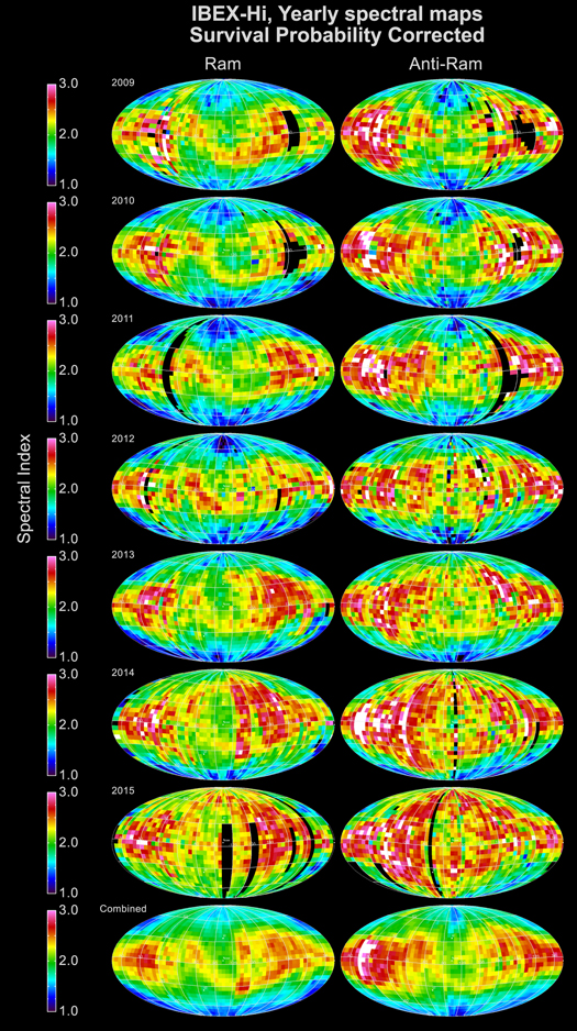
Figure 1. Spectral indices of IBEX observations of ENAs from the first 7 years of observations. Spectral indices are calculated over the energy range of 0.71–4.29 keV, in the spacecraft "ram" (left) and "anti-ram" (right) frames. From McComas et al. (2017).
Download figure:
Standard image High-resolution imageThe ram motion of the IBEX spacecraft introduces a change in the observed latitude of the incoming ENAs of <4° for energies >1 keV (McComas et al. 2010). Since this is less than the ∼6 5 FWHM (full-width at half-maximum) of the IBEX-Hi collimator (Funsten et al. 2009a), and any corrections may introduce more uncertainties in the analysis, it is sufficient to use the latitudinal information in the ram spacecraft frame. The spectral indices shown in Figure 1 are computed for each pixel in the sky without correcting for the change in latitude due to the ram motion of the spacecraft. However, the energy of the incoming ENA also changes when transforming from the spacecraft frame to the inertial frame. The energies are straightforward to correct for the analyses in this paper, where the biggest changes (<14%, for energies >1 keV) occur at the lowest latitudes.
In the first four years of observations (2009–2012), the spectral index is relatively easy to distinguish between low values (<1.5) at high latitudes and higher values at low latitudes. This is due to differences in the source plasma in the inner heliosheath originating from fast or slow solar wind (McComas et al. 2013). However, in 2014–2015 the spectral indices increased at high latitudes. As discussed by McComas et al. (2017), this is likely a response of the closing of the PCHs near solar maximum in cycle 24, resulting in a disappearance of the fast solar wind, and thus a steeper ENA spectrum at high latitudes. Considering this unique correlation between ENA spectral index and solar wind speed, supported by several previous studies, we now examine how well the observed ENA spectra evolve over time with the solar wind speed structure.
In situ observations of the solar wind are difficult to make on a global scale, especially outside of the ecliptic plane. However, remote observations of IPS close to the Sun allow us to determine the solar wind speed (e.g., Kakinuma 1977; Asai et al. 1998; Tokumaru et al. 2010, 2012; Sokół et al. 2013, 2015). The evolution of the solar wind speed at 1 au reconstructed from IPS observations is shown in Figure 2, from Sokół et al. (2015). The solar wind speed evolves similarly in the northern and southern latitudes during most of the solar cycle, but there is a clear temporal difference in the appearance and disappearance of fast solar wind streams in the northern and southern hemispheres. Hemispheric asymmetries in the northern and southern polar winds have been observed by Ulysses (e.g., Ebert et al. 2013), in observations of IPS (e.g., Tokumaru et al. 2015, 2017), and have been applied in global models of the heliosphere (e.g., Pogorelov et al. 2013). This difference manifesting as a shift in the solar maximum peak in the northern and southern hemispheres is related to an asymmetric evolution of the solar magnetic fields during the solar cycle (e.g., Chowdhury et al. 2013, see also discussion in Bzowski et al. 2003). The asymmetry in the solar wind structure as a function of heliographic latitude affects the ENA flux observed by IBEX and is crucial for interpreting IBEX observations during and after solar cycle 23 (as discussed by McComas et al. 2014).

Figure 2. Solar wind speed as a function of heliographic latitude (vertical axis) and time (horizontal axis) reconstructed from IPS observations (Sokół et al.2015).
Download figure:
Standard image High-resolution imageFast (>650 km s−1) solar wind is emitted from the Sun at latitudes ≳30° during solar minimum (centered near ∼1996 and ∼2008), but then the fast solar wind is emitted at high latitudes and eventually disappears as the PCHs shrink near solar maximum (∼2001, ∼2014; see also Karna et al. 2014). As we will show in Section 3, changes in the boundary between fast and slow solar wind streams over time results in a similar response in the ENA spectra as a function of latitude, although delayed in time. The fast and slow solar wind streams create different ENA spectra as higher Mach number solar wind plasma downstream the termination shock results in flatter proton (and thus ENA) spectra in the ∼keV energy range (see, e.g., Wu et al. 2010 for simulation; see Dayeh et al. 2012 for observation).
3. Analysis
3.1. Global ENA Spectral Indices
Figure 3 shows all-sky maps of ENA spectral indices (γ) observed at 1 au computed over the ENA energy range of 0.71–4.29 keV. Here we present ENA spectral indices that are computed from ENA fluxes time-averaged over three periods: 2009–2011, 2012–2013, and 2014–2015. These time periods are chosen for illustration based on the analyses of McComas et al. (2017), who found that significant time variations occur in 2–3 year periods, and the most significant change in ENA fluxes occurs in 2014–2015. However, we note that the results presented later in our paper are derived from analyzing the data on a year-by-year basis.
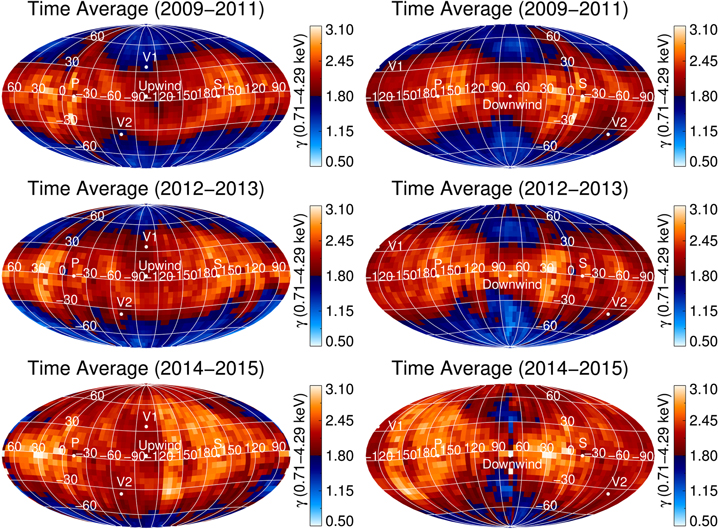
Figure 3. Time-exposure combined maps of spectral index for years 2009–2011 (top), 2012–2013 (middle), and 2014–2015 (bottom). The spectral index is calculated over the entire IBEX-Hi energy range (0.71–4.29 keV). Maps in the left column are centered on the upwind direction, while maps in the right column are centered on the downwind direction. Note that the color bar switches from red (>1.8) to blue (<1.8) to indicate the difference between ENA fluxes produced from slow solar wind at low latitudes and fast solar wind at high latitudes, respectively.
Download figure:
Standard image High-resolution imagePixels with γ < γc = 1.8 are mapped to a blue color scale, and those with γ > γc = 1.8 are in a red color scale. We choose a "critical" index (γc) value of 1.8 since it lies in between ENA spectra with flat (<1.5) and steep (>2) slopes. This value is also close to that found by Livadiotis et al. (2011), who separated the global sky into spectra that can (slow solar wind) or cannot (fast solar wind) be represented by a single kappa distribution, as a possible identifier for fast solar wind PUI distributions downstream of the termination shock (see also Dayeh et al. 2012). In fact, we will show later that spectra at latitudes above and below this critical index are well correlated with the distribution of solar wind speed at similar latitudes.
In Figure 3, ENA spectra from 2009 to 2013 are much flatter at high latitudes than at low latitudes (McComas et al. 2012, 2014, 2017). The ribbon is somewhat identifiable in the maps (most clear in the upper left panel), although having a similar spectral index as the surrounding GDF. However, this behavior is disrupted in 2014–2015, as spectra with γ > 1.8 appear at nearly every pixel, except (1) at latitudes <−60° in the southern hemisphere, and (2) at ∼30°–45° north and south of the downwind direction.
The first condition (persistence of low spectral indices at latitudes <−60° in the southern hemisphere) is likely caused by temporal asymmetries in the evolution of the northern and southern PCHs, and thus fast solar wind streams flowing out from the Sun (this is demonstrated in Section 3.2). As seen in Figure 2, while the fast solar wind flowing from the Sun at high northern latitudes decreased significantly before ∼2012, fast solar wind persisted at high southern latitudes for another year. The second condition (persistence of low spectral indices ∼30°–45° north and south of the downwind direction) is partly caused by the fact that ENA fluxes observed from near the heliotail are produced farther away, with larger line-of-sight integration distances (e.g., Schwadron et al. 2011, 2014; Zirnstein et al. 2016a, 2017). Thus, while solar maximum conditions have begun to be reflected in ENAs from most of the sky in 2014–2015, fluxes from the heliotail originate farther back in time and have not yet "caught up" with changes in the solar wind observed at 1 au. Second, the pixels with γ < 1.8 at ∼30°–45° north and south of the downwind direction are produced in the "north" and "south" heliotail lobes (McComas et al. 2013; Zirnstein et al. 2016a), originating from the fast solar wind propagating through the heliotail (e.g., Pauls & Zank 1996; Pogorelov et al. 2013, 2015; Zirnstein et al. 2017). The fast solar wind is hotter than the slower solar wind at lower latitudes, potentially reducing the ENA spectral index observed at 1 au from these directions.
For a given longitude, most pixels with γ < 1.8 are above a certain latitude, and those with γ > 1.8 are below that latitude. Thus, at any longitude, we can track this "latitudinal boundary" that separates the red (γ > 1.8) and blue (γ < 1.8) pixels, as a function of time. To do this, for any measurement time between 2009 and 2015 we identify this latitudinal boundary by running a 3 pixel boxcar average of spectral index in latitude in an IBEX all-sky map. Starting at the equator, we shift the boxcar in positive (or negative) latitude until it crosses γc. Below we will show that spectra at latitudes above and below this critical index are well correlated with the distribution of solar wind speed at similar latitudes.
An example of ENA spectral variation with latitude is shown in Figure 4, where we show the spectral index averaged over a number of pixels as a function of latitude (7 pixels in longitude, near the nose) in 2009–2011, 2012–2013, and 2014–2015 (middle-left panel). In 2009–2011, the low spectral indices reach the lowest latitudes. There appears to be a double-humped feature on either side of 0° latitude, at least in 2009–2011 and 2014–2015. The local peak at negative latitudes (−30°) is the ribbon, which reaches down to −30°–40° latitude at this longitude. In 2012–2013, the higher spectral indices spread to higher latitudes in the northern hemisphere, but do not change significantly in the south. Finally, in 2014–2015, the low spectral indices largely disappear in the north, but remain in the south at latitudes <−60°. Since the ribbon flux is insignificant at negative latitudes poleward of −45°, the change observed in ∼2014–2015 in the northern hemisphere but not the south is likely due to temporal asymmetries in the solar wind emitted from the northern and southern hemispheres of the Sun.

Figure 4. Example of spectral indices as a function of ecliptic latitude. The spectral indices in the middle-left panel are computed from time-averaged data in periods 2009–2011, 2012–2013, and 2014–2015, in the longitude range of −123° ± 21° (shifted ∼20° starboard of the upwind direction) from the maps in the right column. The critical spectral index γc is shown as the vertical dashed gray line in the middle-left panel. By shifting a 3 pixel boxcar from the equator to each of the poles (leftward and rightward in middle-left panel), the latitude at which the boxcar-averaged spectral index drops below γc is identified as the "boundary" between ENAs of slow (γ > γc) and fast (γ < γc) solar wind origin. This boundary is shown in the right panels as a gray line for each time period. Simulated examples of the solar wind (SW) speed and temperature properties near solar minimum (top) and maximum (bottom) in the northern hemisphere are shown in the top-left and bottom-left panels (from Zirnstein et al. 2015b, 2017).
Download figure:
Standard image High-resolution imageThe double-humped feature in ENA spectral index observed as a function of latitude near the nose of the heliosphere (see middle-left panel of Figure 4) is likely an effect of the plasma properties downstream of the termination shock. Figure 5 shows model results of ENA spectral indices from Zirnstein et al. (2017), at the same ENA energies as the data shown in Figure 4 during 2009–2011. As one can see, there is a visible decrease in ENA spectral index near, but slightly below, the nose direction of the heliosphere. The right panel is a vertical slice of the spectral indices at longitudes similar to those from Figure 4. The decrease in spectral index near the nose of the heliosphere is caused by a significant particle partial pressure near the stagnation region of the heliosphere. This plasma pressure enhancement, identified in MHD simulations (Pogorelov et al. 2011) and observed in ENA data (McComas & Schwadron 2014), results in a smaller ENA spectral index in the ∼keV energy range, and produces the apparent double-humped signature in IBEX ENA spectral index data.
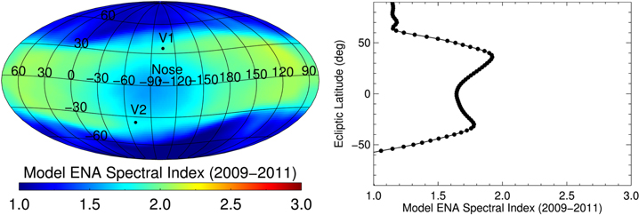
Figure 5. Model of ENA spectral indices from Zirnstein et al. (2017). (Left) All-sky map of ENA spectral indices in the energy range 0.71–4.29 keV, time-averaged from 2009 to 2011. (Right) Spectral index averaged in longitude −123° ± 21° (the same direction as Figure 4) from the left panel. This model demonstrates how the double peaks in ENA spectral index observed in IBEX ENA data (Figure 4) at the fast–slow solar wind boundary is actually caused by a decrease in the ENA spectral index near the nose of the heliosphere.
Download figure:
Standard image High-resolution image3.2. IBEX Observes the Sun's Fast Polar Wind North–South Asymmetry
The results so far strongly suggest that the latitudinal boundary between ENA spectral indices above and below γ ∼ 1.8 are directly caused by the latitudinal-dependent fast and slow solar wind structure emitted by the Sun. This result is demonstrated in Figure 6. In the first panel, we show solar wind speed structure as a function of heliographic latitude at 1 au, after the reconstruction by Sokół et al. (2015), and overplot the latitude at which the ENA spectral index changes from below to above 1.8, from pixels centered on −123° longitude for the north and −81° longitude for the south. The uncertainties are computed by (1) assuming a standard error of 9° for the latitudinal boundary location for each longitude pixel (the boundary was found by a 3 pixel running average, so since each pixel is 6°, the estimated error is ≅3 × 6°/2 = 9°), (2) propagating this error through the pixels averaged in the longitudinal range of −123° ± 21° or −81° ± 21°, and (3) including the standard error of the values about the mean. The time stamps for the IBEX observations are corrected for the delay time of 2.4 years as described in Table 1. Note that the time stamps for the northern and southern IBEX data are not the same since the pixels chosen for the north and south have different longitudes (to avoid the ribbon), and thus, different IBEX measurement times. The ENA results were also calculated for γc = 1.7 and 1.9, although they are not plotted. They yielded similar results to γc = 1.8, especially during the transition to higher latitudes after ∼2011.
Table 1. Estimates of Time Delay between Solar Wind Measured at 1 au and ENA Detection by IBEX
| Line-of-sight Direction | Distance from 1 au to TS (au)a | Distance from TS to RENA (au)b | SW time from 1 au to TS (year)c | SW time from TS to RENA (year)d | ENA time from RENA to 1 au (year)e | Total Time (year)f |
|---|---|---|---|---|---|---|
| Front | 100 | 15 | 0.7 | 0.7 | 0.9 | 2.4 |
| Side | 125 | 30 | 0.9 | 1.4 | 1.3 | 3.6 |
| Back | 175 | 50 | 1.3 | 2.4 | 1.8 | 5.5 |
Notes. Distances to the termination shock (TS), average ENA source region (RENA), and solar wind (SW) speeds change over time, thus the values in this table are approximations of the average. All distances are assumed to be radial. Note that the estimates for the side and back directions of the heliosphere are not used for analyses in this paper, they are merely provided for perspective.
aDistances to the termination shock are chosen based on Voyager observations (Stone et al. 2005, 2008) for the front of the heliosphere, and the model by Zirnstein et al. (2016a) for the side and back. We use the "front" direction to estimate the time delay of ENAs measured near the nose longitude, at any given latitude. Thus, the value for the distance to the termination shock in the front of the heliosphere is chosen to be larger than the values observed by Voyagers 1 and 2 to account for larger distances to the shock expected at higher latitudes. bRENA designates the average distance beyond the termination shock within which most ENAs visible by IBEX originate. Estimates are taken from Voyager 1 data and Zirnstein et al. (2016a). cSupersonic SW speed is assumed to be 650 km s−1, which is a reasonable choice for the transition between slow and fast SW (McComas et al. 2000). dThe inner heliosheath plasma speed is assumed to be 100 km s−1. eENA speed is assumed to be that of a 1.74 keV ENA (∼577 km s−1). fTotal time delay between solar wind measurement at 1 au and ENA measurement at 1 au.Download table as: ASCIITypeset image
The latitude of IBEX ENA spectra match well with the transition between slow and fast solar wind over time. We observe an asymmetry in the evolution of the ENA spectral indices in the northern and southern hemispheres. The boundary between low and high spectral indices observed by IBEX in the northern hemisphere reaches higher latitudes before it does in the south. This temporal asymmetry is also observed in solar wind speed, where Figure 6 shows that the fast solar wind disappears at high northern latitudes ∼1 year before the south. Moreover, this temporal asymmetry is also seen in extreme-ultraviolet (EUV) observations of the PCH areas made by the Extreme-ultraviolet Imaging Telescope on the Solar and Heliospheric Observatory and the Atmospheric Imager Assembly on the Solar Dynamic Observatory (Karnaet al. 2014). Reisenfeld et al. (2016) found that the evolutionary trend of ∼4 keV ENA intensity from the poles correlated well with that of the Sun's PCH fractional areas.
We also note that Ulysses data have shown that the solar wind becomes highly variable, with fast and slow solar wind stream interactions, during solar maxima (e.g., Ebert et al. 2013). From our analysis, it appears that we are able to identify and follow the trend of the fast–slow solar wind boundary in ENA spectra (although delayed in time) as the solar cycle approaches solar maximum. It appears unlikely that we would be able to identify small polar coronal holes near the Sun's poles at solar maximum, but our analysis shows that we can see the closing, and likely the opening, of polar coronal holes below ∼75° latitude. The solar wind composition (e.g., density, temperature) is also useful for differentiating the fast and slow solar wind, which has been done previously (e.g., Ebert et al. 2009), but our analysis shows that the solar wind speed is sufficient for our purposes.
While our results compare relatively well with the temporal trends of the solar wind speed, in ∼2009–2011 the ENA results appear to deviate significantly in the southern hemisphere. This may be partly attributed to ENA flux from the ribbon interfering with the determination of the fast–slow solar wind latitude boundary in the southern hemisphere (−81° longitude). However, we also note that the reconstruction of solar wind speeds derived from IPS observations from Sokół et al. (2015) is less certain due to a lack of IPS measurements in 2010.
To demonstrate the similarities between our ENA observations with EUV observations of the PCH areas, in Figure 7, we converted the fast–slow solar wind latitudinal boundary from IBEX observations to a fractional solid angle of fast polar solar wind centered on the Sun's rotational poles. This is done by assuming the latitude at which the transition between slow and fast solar wind is observed in IBEX ENA data from near the nose (using spectral index γ ∼ 1.8) is a realistic marker of the supersonic solar wind fast–slow solar wind boundary. This is true if the line-of-sight-integrated ENAs downstream of the termination shock do not originate from streamlines connected to the termination shock at significantly different latitudes. Since most ENAs observed by IBEX originate closer to the termination shock than farther away due to the extinction of energetic proton distribution (e.g., Zirnstein et al. 2016a), this is a decent, zeroth-order assumption for our purposes.

Figure 6. (Left) solar wind speed (color bar) and the fast–slow solar wind boundary determined from IBEX ENA data (black symbols). The IBEX data are taken from near the nose (upwind) direction centered at −123° ± 21° longitude for the northern latitudes and −81° ± 21° longitude for southern longitudes, to avoid the ribbon as best as possible (both are shifted ∼20° in longitude from the nose direction). The ENA results are time-corrected for solar wind and ENA propagation (see Table 1) to plot in the solar wind measurement time (x-axis). (Right) comparing the fast–slow solar wind boundary derived from IBEX ENA data in the northern and southern hemispheres for γc = 1.8, in the ENA measurement time.
Download figure:
Standard image High-resolution imageWe derive the polar fast solar wind fractional solid angle from IBEX observations by converting the latitudinal boundaries shown in Figure 6 to the solid angle of a spherical cap centered at the northern solar pole, divided by 4π. For example, IBEX data from the northern hemisphere in Figure 6 show a latitude of ∼40° in the first few years. We convert this to the solid angle of a spherical cap using  , where θ is latitude. By dividing this by 4π, this yields the fraction of the solid angle in the sky of the polar fast solar wind, approximated from IBEX ENA observations. Then, we divide this value by the solar magnetic flux-tube expansion factor, giving the results shown in Figure 7. The solar magnetic flux-tube expansion factor is typically determined to be between ∼10 and 7 for solar wind speeds from ∼550–650 km s−1, and between ∼7 and 4.5 for speeds 650–750 km s−1, respectively (e.g., Wang & Sheeley 1990, 2006; Wang et al. 1997; Arge & Pizzo 2000). Since we are tracking the boundary of the fast solar wind, which we take to be about ∼650 km s−1 (e.g., McComas et al. 2000, 2008), the expansion factor is likely about 7. However, we find that dividing the IBEX results by 5, instead of 7, gives a better comparison to the PCH surface area. This difference may be due to (1) inaccuracies in converting ENA spectral index latitude to fast–slow solar wind boundary latitude, or (2) the choice of expansion factor depends more on the average polar fast solar wind speed, rather than the speed at the fast–slow solar wind boundary, which will produce an expansion factor closer to 5. Regardless of this choice, the relevant trends will not change.
IBEX data in the northern hemisphere match the PCH fractional area data well, given the simple time-delay estimates we chose from Table 1. We point out that while the IBEX-derived fast solar wind solid angle approaches ∼0% before 2012, the PCH data derived from EUV observations only reach a minimum of ∼0.5%, which Karna et al. (2014) point out is likely the noise floor of the data. While the IBEX data in the southern hemisphere appears to be evolving slightly ahead of the PCH data, this is likely partly due to small differences in the actual ENA delay time in the southern hemisphere of the outer heliosphere compared to what we estimated. For example, we estimated that the flow speed in the inner heliosheath was 100 km s−1. A decrease in speed of 40 km s−1 in the southern hemisphere would produce a difference in time delay of ∼6 months, which could explain the time discrepancy with the southern PCH data. Another difference would be shorter distances to the termination shock, heliopause, or average ENA source distance due to a stronger compression of the interstellar magnetic field on the heliopause in the southern hemisphere.
3.3. IBEX ENA Spectra from the Flanks and Tail
In the previous section, we examined ENA spectra from near the nose of the heliosphere. However, since the distance to the termination shock and the depth of the heliosheath are larger near the tail-ward side of the heliosphere, we expect to see different temporal trends in ENA fluxes observed near the flank and tail directions since the plasma and ENAs will take a longer amount of time to propagate through the heliosphere. In Figure 8, we show the latitudinal boundary of high versus low spectral indices determined from the port/starboard lobe directions and the tail ("port" and "starboard refer to the left- and right-hand sides of the heliosphere, from the point of view of an observer centered at the Sun; the lobes are identified in McComas et al. 2013; Zirnstein et al. 2016a). For the port/starboard lobes, we only show results from the southern hemisphere to avoid the ribbon in the northern hemisphere at these longitudes. As one can see, from 2009 to ∼2011 the latitudinal boundary decreases in the port and starboard flanks, remains steady for a few years, then begins increasing to higher latitudes after 2014. The initial decrease (especially from the port lobe) is not observed in spectra from the nose direction. This indicates that the fluxes are delayed in time from the port/starboard lobe directions more than in the nose direction, such that we can observe part of the approach of solar cycle 23 to solar minimum in ∼2007–2008, but reflected in ENA observations a few years later.

Figure 7. Fractional solid angle of the fast solar wind emitted from the Sun derived by IBEX ENA data from Figure 6, as well as the fractional surface area of the PCHs derived from EUV observations (Karna et al. 2014). The solid angles from IBEX data are derived by (1) converting the latitudinal boundary shown in Figure 6 to the solid angle of a spherical cap centered at the northern solar pole, divided by 4π, and (2) accounting for the solar magnetic flux-tube expansion factor, which we take to be 5. The PCH data from Karna et al. (2014) are smoothed with a running boxcar with a width of 13 Carrington rotations (∼1 year) to match IBEX data cadence and to reduce annual systematic variations.
Download figure:
Standard image High-resolution imageThere appears to be a small difference in this boundary from the port and starboard directions, where the spectra from the port lobe direction are slightly lagging the starboard spectra. Since we are analyzing fluxes from the same (southern) hemisphere, but significantly different longitude (∼108° apart), these results suggest possible asymmetries in the heliospheric structure on either flank side of the heliosphere, such as (1) the distances to the termination shock, (2) the thickness of the inner heliosheath, or (3) the charge-exchange rate and effective distance of the ENA source region. If fluxes from the port side of the heliosphere are truly lagging, the starboard fluxes, this suggests the ENA source distance is closer on the starboard (i.e., closer distance to the termination shock and/or heliopause) or perhaps that the rate of charge-exchange is higher in the starboard heliosheath, effectively reducing the distance ∼keV protons travel before being converted to ENAs. Both are consistent with a larger external pressure induced by the interstellar magnetic field on the starboard side of the heliosphere.
In the tail direction, the latitudinal boundary separating the high and low ENA spectral indices is significantly lower than near the flanks and nose, and does not change as much over time. This is due to the longer distance at which ENAs are created in the tail direction. Previous studies have estimated this "cooling depth" distance from the heliotail direction (Schwadron et al. 2011, 2014; Galli et al. 2016; Zirnstein et al. 2016a). Each of these studies utilized different energy ranges of the ENA spectrum to derive effective distances to the ENA heliotail source region. Zirnstein et al. (2016a) analyzed the highest ENA energies only, resulting in a shorter cooling depth due to the energy-dependent, charge-exchange rate (∼70–100 au). Schwadron et al. (2014) included a lower range of ENA energies, resulting in a larger distance (∼100–170 au). Galli et al. (2016) derived an effective distance at which ENAs are observed based on the line-of-sight-integrated pressure with ENA energies as low as ∼0.015 keV, resulting in the largest (average) distance (220 ± 110 au). Overall, the results of each analysis are consistent with each other considering the different approaches, estimates (e.g., distance to the termination shock, plasma flow speed), and ENA energy ranges utilized in their analyses. Based on these analyses, the data shown in the right panel of Figure 8 show the ENA fluxes must indeed be generated farther from the Sun than the nose or flank spectra (the lower latitude of the boundary indicates a farther source), and that the less significant changes in the northern and southern boundaries suggest a longer integration distance, effectively smoothing out variations in the solar wind.
3.4. Correlation between IBEX ENA Spectra and Solar Wind Speed Distributions
Not only does the boundary separating ENA spectra with low and high spectral indices follow the fast–slow solar wind structure observed at 1 au, but the distribution of the ENA spectral indices above and below those latitudes are directly related to the solar wind speed distribution. In Figure 9, we show histograms of the ENA spectral index at all positive/negative latitudes above (blue) and below (green) the critical latitude λc defined by a spectral index γc = 1.8.
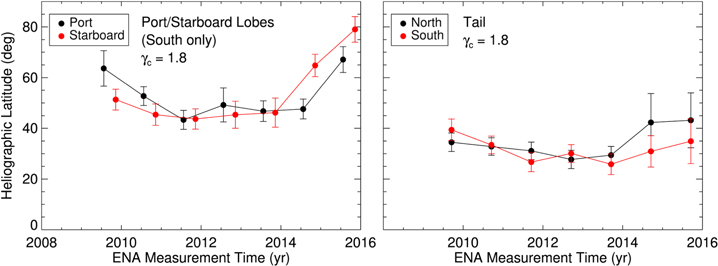
Figure 8. Comparing the fast–slow solar wind boundary derived from IBEX ENA data near the port/starboard lobe directions (left) and the downwind/tail direction (right). We choose directions within 21° ± 21° longitude for the port lobe and 129° ± 21° for the starboard lobe. Both are centered ∼55° from the downwind/tail direction. Note that since the ribbon crosses the northern hemisphere of the port and starboard lobes, we only analyze the southern hemisphere in the left panel.
Download figure:
Standard image High-resolution image
Figure 9. (Left) Histogram of ENA spectral indices taken from ecliptic longitudes −123° ± 21° in the northern hemisphere and −81° ± 21° in the southern hemisphere, for ecliptic latitudes above and below the spectral latitude boundary defined by γc = 1.8. Shown are results over time periods of 2009–2011 (top), 2012–2013 (middle), and 2014–2015 (bottom). (Right) Histogram of solar wind speeds at heliographic latitudes above ("fast SW") and below ("slow SW") the latitude defined by a solar wind speed = 650 km s−1. The speeds are taken from a time range that takes into account the delay for solar wind and ENA propagation (Table 1), and the time at which ENAs were observed. The same time corrections are done for each row. Note that the ENA data are computed in ecliptic coordinates, while SW data are in heliographic coordinates. Converting the ENA latitudinal boundary to heliographic coordinates before computing the histogram does not significantly change the results, since the ecliptic axis is only ∼7° from the heliographic axis.
Download figure:
Standard image High-resolution image
For the northern latitudes, we take a histogram in a 7 pixel longitude range to the starboard side of the nose of the heliosphere (centered on −123° longitude, ∼19° from the nose direction). For the southern latitudes, to avoid the ribbon, we take a histogram in a 7 pixel longitude range to the port side of the nose (centered on −81° longitude, ∼23° from the nose direction). These regions are the same as those used in Figures 6 and 7. We also show histograms of the solar wind speed, but delayed in time (see the description below). Similar to how we separate ENA spectral indices into high and low latitude regions, we separate the solar wind speed into regions of high latitude "fast" (red) and low latitude "slow" (yellow) solar wind. We use a 3 pixel running boxcar technique similar to that used for the ENA spectral index, but using a critical solar wind speed of 650 km s−1 to define the "boundary" between fast and slow solar wind (McComas et al. 2000, 2008).
To directly compare ENA spectral indices observed at 1 au by IBEX to solar wind speeds observed derived from IPS, we must account for the time it takes the solar wind to propagate to the outer heliosphere and ENA propagation back to 1 au. Therefore, in the left panels, we show IBEX observations at their measured times, and in the right panels show solar wind speed observations earlier in time using a delay time estimate shown in Table 1 for the noseward side of the heliosphere (∼2.4 years). We then add an uncertainty of 50% for this delay time to account for uncertainties in knowing the exact distances to the termination shock and heliopause, and the longer time it takes for solar wind and ENAs to travel between the heliosheath and 1 au at higher latitudes. We subtract this delay time from the IBEX observational periods (2009–2011, 2012–2013, and 2014–2015) to obtain the temporal periods of solar wind observations that should be compared to IBEX data. For example, for the IBEX observational period 2009–2011, accounting for the fact that the pixels we are analyzing are taken at a specific time during this period (2009.22–2011.22), the solar wind speeds at 1 au are taken between 2009.22–1.5 × 2.4 ≃ 2005.6, and 2011.22–0.5 × 2.4 ≃ 2010. The same delays are then applied to the second and third IBEX observational periods.
Figure 9 shows that the evolution of the IBEX ENA spectral index distribution in the ∼0.7–4.3 keV energy range correlates well with IPS-observed solar wind speed distribution. During the first few years of IBEX observations, ENA spectra with γ < 1.8 (i.e., at high latitudes) are centered near γ ∼ 1.5 (see the mode and FWHM properties of the histograms in Table 2). ENA spectra above 1.8 (i.e., at low latitudes) are centered near γ ∼ 2.0. As indicated by previous studies, these conditions are caused by differences between fast solar wind at high latitudes (with higher Mach number and hotter plasma, producing higher energy ENAs downstream of the termination shock) and slower solar wind at low latitudes (a lower Mach number and relatively cooler plasma, producing lower energy ENAs downstream of the termination shock; e.g., Wu et al. 2010; Zank et al. 2010; Zirnstein et al. 2017). Similar behavior of the solar wind is demonstrated in the right column, with fast solar wind (∼700 km s−1) at high latitudes correlating with ENA spectra of γ ∼ 1.5, and slow solar wind (∼500 km s−1) at low latitudes correlating with ENA spectra of γ ∼ 2.0.
Table 2. Properties of ENA Spectral Index and SW Speed Histograms from Figure 8
| Period (year) | Latitude (degree) | Mode | FWHM | |
|---|---|---|---|---|
| ENA Spectral Index | 2009–2011 | λ > λ(γ = 1.8) | 1.47 | 0.41 |
| λ < λ(γ = 1.8) | 1.99 | 0.50 | ||
| 2012–2013 | λ > λ(γ = 1.8) | 1.37 | 0.49 | |
| λ < λ(γ = 1.8) | 2.08 | 0.56 | ||
| 2014–2015 | λ > λ(γ = 1.8) | ⋯ | ⋯ | |
| λ < λ(γ = 1.8) | 2.11 | 0.49 | ||
| SW Speed (km s−1) | 2005.6–2010 | λ > λ(v = 650) | 699 | 143 |
| λ < λ(v = 650) | 514 | 201 | ||
| 2008.6–2012 | λ > λ(v = 650) | 691 | 143 | |
| λ < λ(v = 650) | 522 | 192 | ||
| 2010.6–2014 | λ > λ(v = 650) | ⋯ | ⋯ | |
| λ < λ(v = 650) | 485 | 161 | ||
Note. The mode and FWHM are found by fitting a Gaussian distribution of the form f ∝ exp[-(x-μ)2/2σ2] to the histograms in Figure 8, where μ is the mode and  . Since the histograms in the high latitude regions (blue for ENA spectra, red for SW speed) in the last row of panels in Figure 9 are highly non-Gaussian and have a low number of occurrences, we do not calculate their mode and FWHM.
Download table as: ASCIITypeset image
As time progressed (2012–2013), the mode of the ENA spectral indices at high and low latitudes did not significantly change (note that the total number of occurrences reduced since this is a 2 year period, compared to a 3 year period for the top panels in Figure 9), while both of their FWHMs slightly increased. Similarly, the solar wind speed modes remained approximately the same as in the previous few years. However, the relative number of occurrences in each population is beginning to invert, with slightly more occurrences in the high ENA spectral index population (green) and slow solar wind speed population (yellow). Finally, in 2014–2015, the number of occurrences of ENA spectral indices below 1.8 decreased significantly, resulting in a substantial number spanning between γ ∼ 1.8–2.5, due to (1) the increase in the critical latitude boundary separating spectra produced by fast and slow solar wind, thus, reducing the number of pixels/occurrences at high latitudes, and (2) a lower number of occurrences of low γ at all latitudes, where the "green" population encompasses nearly all latitudes. This directly correlated with the change in solar wind ∼2–3 years prior, with a global decrease in solar wind speed at high latitudes.
The mode of the ENA spectral index distribution is related to a specific range of solar wind speeds. For example, in 2009–2011, the modes of the ENA spectral index distributions are near ∼2.0 and 1.5 at low and high latitudes, respectively, while the solar wind speed was ∼500 and ∼700 km s−1, at similar latitudes. In 2014–2015 the mode of the ENA spectral index distribution over most of the sky is ∼2.1. This corresponds to a dominant solar wind speed of ∼485 km s−1. Thus, it is not surprising that the speed of the solar wind is directly responsible for the ENA spectral characteristics produced downstream of the termination shock. The fast solar wind at high latitudes produces a hotter and flatter proton spectrum downstream of the termination shock, resulting in a flatter ENA spectrum.
4. Discussion and Conclusion
In this study, we utilized IBEX observations of ENAs in the energy range of 0.71–4.29 keV to derive a latitudinal boundary separating spectra with high and low indices (Figures 3–4), which appears well correlated with the boundary separating fast and slow solar wind emitted from the Sun (Figure 6). During the first 5 years of observations (2009–2013), IBEX shows ENA spectra with a significantly lower index at high latitudes than at low latitudes, where the source plasma is dominated by faster (and hotter) solar wind originating from the PCHs. Upon crossing the termination shock, the fast solar wind plasma produces a proton population that is significantly hotter than the plasma from slow solar wind at lower latitudes, effectively reducing the average observed ENA spectral index. In the last few years, however, the latitudinal boundary signifying the fast–slow solar wind boundary had increased to higher latitudes, indicating the disappearance of the PCHs as the solar wind progressed toward solar maximum conditions in cycle 24 (Figure 7). The correlation between the averaged ENA spectral index and the solar wind speed is further supported by the comparison between histograms of ENA spectral indices and solar wind speeds above and below similar latitudes, linking a specific range of ENA spectral indices to a range of solar wind speeds (Figure 9).
IBEX observations also show a significant temporal asymmetry in the evolution of the boundary separating low and high spectral indices near the nose of the heliosphere, with the spectra in the northern hemisphere increasing in spectral index at higher latitudes before the southern hemisphere (Figure 6). This is consistent with the solar wind speed at 1 au derived from IPS observations (Sokół et al. 2015; Tokumaru et al. 2015), as well as EUV observations of the northern and southern PCH fractional areas (Karna et al. 2014; Reisenfeld et al. 2016; Tokumaru et al. 2017). This correlation strongly supports the idea that the average spectral index observed by IBEX in the ∼0.7–4.3 keV energy range reflects the average solar wind speed that created it, as well as the fact that the heliosphere structure in the northern and southern hemispheres near the nose of the heliosphere is not significantly different as to distort this asymmetry. However, the accuracy of this analysis may not be sufficient to identify asymmetries of the heliosphere close in longitude and latitude, so any small differences that may exist in the heliospheric structure near the nose (such as that identified by Voyager 1 and 2), may not be visible in our analysis.
We also note the possible limitations in comparing our ENA results to the reconstructed solar wind speed model. The model may not resolve small-scale transients, but these are unlikely to affect our line-of-sight-averaged ENA results. While it is difficult to quantify the uncertainties in the reconstructed solar wind speed, comparisons with Ulysses solar wind speed measurements revealed reasonable agreement with the model (average ∼20% difference; Sokół et al. 2015). Though our latitudinal boundary results derived from IBEX ENA data are based on choosing a critical spectral index (γc ∼ 1.8) to identify the fast–slow solar wind boundary, the derivation of the latitudinal boundaries from the ENA data is independent of the solar wind speed model, and the general agreement between the ENA and solar wind speed data (e.g., Figure 6) supports the link between ENA spectral index and the supersonic solar wind speed structure.
Our results also reproduced the fractional surface area of the PCHs from the last 7 years (Figure 7) reasonably well. While the comparison is good, we note a few uncertainties in deriving the fast solar wind fractional area from IBEX data. The first is that, as the Sun rotates, fast solar wind emitted from the PCHs, which is not likely to be symmetric about the Sun's rotation axis, will propagate through space and fill a larger solid angle in space that is more symmetric about the Sun's rotation axis, and project a surface area that is larger than the original PCH area. While we did account for the expansion of the polar coronal fast solar wind from the solar surface, we expect that the PCH fractional area should still be smaller owing to the rotation of the Sun and the angle between the solar rotation and magnetic axes (i.e., the current sheet tilt angle; see Wilcox Solar Observatory data, http://wso.stanford.edu). However, the current sheet tilt angle is small during solar minimum (∼10°), when this effect would be most important.
Moreover, our analysis assumes that the line-of-sight-integrated ENAs downstream of the termination shock do not originate from streamlines connected to the termination shock at significantly different latitudes. We argue that since most ENAs observed by IBEX originate closer to the termination shock than farther away due to the extinction of energetic proton distribution (e.g., Zirnstein et al. 2016a, 2017), this will reduce the chances for observing a significant number of ENAs originating from multiple streamlines at different latitudes. However, this can be quantified more carefully using global time-dependent simulations of the heliosphere, and should be analyzed in a future study.
Our results suggest that the temporal evolution of ENAs from the port and starboard flanks (where ENAs from the port lobe may be lagging fluxes from the starboard lobe) of the heliosphere may be slightly different due to a structural asymmetry in the outer heliosphere rather than in the solar wind emitted from the Sun. While it is difficult to definitively prove this asymmetry due to our 1 year time cadence and statistical uncertainties, if true, this behavior would suggest the following: (1) the distance to the line-of-sight-averaged ENA source may be closer in the starboard lobe direction (i.e., distance to the termination shock or heliopause), and/or (2) the charge-exchange rate is significantly higher in the starboard side of the heliosphere, effectively reducing the time it takes to convert ∼keV protons to ENAs. The line-of-sight-integrated partial pressures (in the 0.71–4.29 keV energy range) derived from IBEX data show a higher partial pressure in the starboard lobe direction of the heliosphere, perhaps induced by the VLISM magnetic field (Schwadron et al. 2014). A higher line-of-sight-integrated partial pressure may indicate a thicker inner heliosheath region, or more literally a higher plasma pressure.
There is no significant difference in the latitudinal boundary between high and low ENA spectral indices from the northern and southern hemispheres in the tail direction. This is not surprising, since variations in ENA fluxes induced by the dynamic solar wind plasma are more likely to be smoothed out in the larger line-of-sight integration down the heliotail. However, the fact that the latitudinal boundary from the tail direction is at a lower latitude (∼30°) compared to the nose or flanks (∼40°) shows that the average ENA source distance must be farther away (or the ENA source region extends farther from the termination shock)—as plasma propagates down the heliotail, from the point of view of an observer at 1 au, the latitude separating ENAs produced from fast versus slow solar wind reduces to lower latitudes. The time-dependent model from Zirnstein et al. (2017) derived a similar latitude from the tail direction (see their Figure 6). Based on their model, the distance within most ENAs originate (i.e., the distance at which 1/e ∼ 63% of observed ENAs originate) is ∼135 au and 65 au for ∼0.7 and 4.3 keV ENAs, respectively. Thus, IBEX observations indicate that most ∼keV ENAs are produced within ∼100 au beyond the termination shock in the tail direction.
This work was carried out as part of the IBEX mission, which is part of NASA's Explorer program. E.Z. thanks Nishu Karna for providing the PCH fractional area data, thanks Jacob Heerikhuisen for providing heliosphere simulation results, and acknowledges helpful discussions with Dan Reisenfeld. Work at SwRI was partially supported by NASA grant NNX17AB98G. J.M.S. acknowledges support by grant No. 2015-19-B-ST9-01328 from the National Science Center, Poland, as well as the Institute for Space-Earth Environmental Research, Nagoya University, Nagoya, Japan for providing the solar wind speed data from IPS observations that were used in the time/latitude reconstruction model in Sokół et al. (2013, 2015).