


Abstract
The OH+ ion is of critical importance to the chemistry in the interstellar medium and is a prerequisite for the generation of more complex chemical species. Submillimeter and ultraviolet observations rely on high quality laboratory spectra. Recent measurements of the fundamental vibrational band and previously unanalyzed Fourier transform spectra of the near-ultraviolet A3Π−X3Σ− electronic spectrum, acquired at the National Solar Observatory at Kitt Peak in 1989, provide an excellent opportunity to perform a global fit of the available data. These new optical data are approximately four times more precise as compared to the previous values. The fit to the new data provides updated molecular constants, which are necessary to predict the OH+ transition frequencies accurately to support future observations. These new constants are the first published using the modern effective Hamiltonian for a linear molecule. These new molecular constants allow for easy simulation of transition frequencies and spectra using the PGOPHER program. The new constants improve simulations of higher J-value infrared transitions, and represent an improvement of an order of magnitude for some constants pertaining to the optical transitions.
Export citation and abstract BibTeX RIS
1. Introduction
Molecular ions play a crucial role in the chemistry of diffuse interstellar clouds (van Dishoeck & Black 1986; Le Petit et al. 2004). The OH+ ion is particularly interesting as it is a critical intermediate in interstellar chemistry. Cosmic ray ionization of H or H2 and subsequent reaction with atomic oxygen are responsible for the generation of OH+, which can undergo further reactions with molecular hydrogen to form H2O+ and H3O+ (Federman et al. 1996; Hollenbach et al. 2012). These species can undergo dissociative recombination with electrons to form the radical OH, which reacts with C or C+ to create CO paving the way for more complex molecules. OH+ is critical for building reaction networks that define interstellar chemistry. As a consequence of these chemical models, OH+ column densities are correlated with those of other molecules such as CH+, and OH column densities are correlated with CN and CH (Porras et al. 2014).
Because the mechanism of formation for OH+ requires cosmic ray ionization, the column density of OH+ relative to the column density of H has been used by Porras et al. (2014), Hollenbach et al. (2012), and Indriolo et al. (2015) to infer the cosmic ray ionization rate, which is key to understanding both the physical and chemical conditions in various interstellar environments. The rate is consistent with other methods to determine the cosmic ray ionization rate, e.g., via  (Indriolo & McCall 2012).
The first astronomical observations of OH+ were realized by Wyrowski et al. (2010) using the Atacama Pathfinder Experiment 12 m telescope toward Sagittarius B2(M). Two hyperfine components of the N = 1−0 J = 0−1 transition of the ground state were observed. Subsequent detections were made with the Herschel Space Telescope's HIFI instrument by Neufeld et al. (2010) and Gerin et al. (2010). Additional detections have been made in the near-ultraviolet (near-UV) with the Ultraviolet and Visual Eschelle Spectrograph of the Very Large Telescope (Krełowski et al. 2010; Porras et al. 2014).
The first laboratory spectrum of OH+ was acquired in the near-UV by Rodebush & Wahl (1933). The transitions observed by Rodebush & Wahl (1933) were assigned to the A3Π−X3Σ− transition by Loomis & Brandt (1936). These authors noted that the A3Π v = 1 level was severely perturbed. The first adequate treatment of the perturbation (due to the b1Σ+ v = 0 state) was by Merer et al. (1975). The first rotational spectroscopy was accomplished in 1985 by Bekooy et al. (1985), who measured the hyperfine components of three transitions in the ground vibronic state. Additional rotational work in the ground state was performed with laser magnetic resonance spectroscopy and laser diode spectroscopy (Gruebele et al. 1986; Liu et al. 1987). The rotational spectrum of the J = 3 − 2 transition of the a1Δ electronic state has also been observed by laser magnetic resonance (Varberg et al. 1994). The fundamental vibrational band was first measured by Crofton et al. (1985), and hot bands were measured shortly thereafter (Rehfuss et al. 1992). Recently, the fundamental band was remeasured by Markus et al. (2016) with greatly improved uncertainty over the earlier measurements.
There have been a variety of predissociation measurements in the excited electronic states, including the A3Π, a1Δ, b1Σ+, and c1Π states. The first was by Helm et al. (1984) who observed a handful of transitions in the (5, 2) and (6, 2) bands in the A3Π−X3Σ− system. The c1Π−b1Σ+ system was first studied by Rodgers & Sarre (1988) and then revisited with additional measurements from the c1Π−a1Δ system (Rodgers et al. 2007).
A Fourier transform spectrum of the OH radical was acquired at the McMath Solar Observatory of Kitt Peak National Observatory in 1989 (Stark et al. 1994). This spectra also contains transitions that are associated with the A–X transition of OH+, which were not analyzed. The present work utilizes that new data along with relevant rotational work (Bekooy et al. 1985; Liu et al. 1987), rovibrational (Rehfuss et al. 1992; Markus et al. 2016), and rovibronic data sets (Rodgers et al. 2007) to perform a combined fit. The resulting molecular constants, including the perturbation, are the most accurate and precise published to date, which allows the prediction of OH+ transitions to better accuracy, thereby supporting observations of OH+ in the interstellar medium. Calculations of the radiative lifetimes, transition dipole moments, and oscillator strengths (Saxon & Liu 1986; Merchán et al. 1991; Gómez-Carrasco et al. 2014; Zhao et al. 2015) are benefited by the low uncertainty line positions and are useful tools for identifying new spectral signatures attributed to OH+ (Zhao et al. 2015). The astrophysical implications will be discussed in greater detail in Section 3.2.
2. Experiment
Near-UV data were collected by the 1 m Fourier transform spectrometer at Kitt Peak in 1989 by J. W. Brault and R. Engleman and published in 1994 (Stark et al. 1994). The spectrum that was obtained targeted the A2Σ+−X2Π transitions of the OH radical, although it also contained transitions from the A3Π−X3Σ− system of OH+. The OH+ transitions have not been analyzed, and they provide an excellent opportunity to improve the molecular constants of the A and X states.
The source for generating the OH and OH+ was an iron-hollow cathode discharge. The discharge cell was filled with a pressure of 2.2 Torr of helium and ∼10 mTorr of H2O. A direct-current (DC) discharge was struck with a voltage of 235 V at a current of 300 mA. The detection was performed using an 8 mm aperture, and the light was detected with silicon photodiodes. A 280–540 nm bandpass was used to select the wavelength region of interest, and the final spectrum is the sum of 8 scans at a resolution of 0.05 cm−1.
3. Results and Discussion
3.1. Spectroscopy Summary
The ground state rotational (Bekooy et al. 1985; Liu et al. 1987) and rovibrational (Rehfuss et al. 1992; Markus et al. 2016) data sets were simulated using SPCAT/SPFIT (Pickett 1991) with the Dunham constants from the Cologne Database for Molecular Spectroscopy (CDMS; Endres et al. 2016). The hyperfine structure was collapsed by setting the splitting parameters to zero. This choice was made to simplify the fitting process because the data from the A–X transition are not hyperfine-resolved and cannot improve these constants. The ground state data were combined with the near-UV data and the predissociation data (Rodgers et al. 2007) and fit in PGOPHER (Western 2017) using the built-in  Hamiltonian for a diatomic molecule (Brown et al. 1979). The ground state data were fit first, relying on the low uncertainty pure rotational and rovibrational data to establish the ground state molecular constants before the attempting to fit the A–X band system.
The simulated rotational and vibrational transition frequencies used to determine the molecular constants are available as supplementary material online as part of the complete Table 2. Initial guesses for the molecular constants were made based on those reported by Rehfuss et al. (1992) and Markus et al. (2016). After the fit converged, the uncertainties of the data set were adjusted to cause the error weighted residuals to be distributed normally. These adjustments generally involved increasing the average error of the data set. No error was reduced below the reported error in the original publication.
The data set by Markus et al. (2016) is partially resolved with respect to the hyperfine components, and the rotational data are fully resolved. As a result of zeroing the hyperfine splitting, the corresponding transition uncertainties are somewhat larger than reported in the original works. The uncertainty for the rotational data was set to 7.5 × 10⁻⁵ cm−1 and the uncertainty used for the fundamental band published in Markus et al. (2016) was set to 3 × 10⁻⁴ cm−1.
The data are fit and the constants are reported in Table 1. The transitions were sequentially fit from the ground state rotational data to the data from the highest vibrational state that had been observed (i.e., each vibrational level was added after a converged fit was achieved). This ladder approach was chosen to ensure the lower level for each vibration was related to the the highest precision data available.
Table 1. Spectroscopic Constants for the X3Σ− Ground State
| Constants | v = 0 | v = 1 | v = 2 | v = 3 | v = 4 |
|---|---|---|---|---|---|
| (cm−1) | (cm−1) | (cm−1) | (cm−1) | (cm−1) | |
| Gv | 0.0 | 2956.358469(84) | 5755.68880(12) | 8404.1646(16) | 10907.94161(22) |
| Bv | 16.422907(11) | 15.6952559(71) | 14.9886184(71) | 14.303262(12) | 13.639476(21) |
| Dv/10−3 | 1.92166(28) | 1.87278(96) | 1.823433(90) | 1.77341(22) | 1.72329(59) |
| Hv/10−7 | 1.315(28) | 1.3018(36) | 1.2614(31) | 1.210(12) | 1.192(43) |
| Lv/10−10 | 0.24(11) | ⋯ | ⋯ | ⋯ | ⋯ |
| Mv/10−13 | −0.56(15) | ⋯ | ⋯ | ⋯ | ⋯ |
| λv | 2.143043(47) | 2.133024(73) | 2.121213(95) | 2.10813(15) | 2.09296(28) |
| λDv/10−5 | −2.40(22) | −2.43(24) | −2.40(24) | −2.93(34) | −2.31(59) |
| γv | −0.151229(18) | −0.146542(18) | −0.141943(20) | −0.137455(30) | −0.133040(46) |
| γDv/10−5 | 2.590(10) | 2.473(14) | 2.349(15) | 2.267(33) | 2.104(62) |
Note. Values in parenthesis represent 1σ standard deviations.
Download table as: ASCIITypeset image
The v = 5 − 4 transition, first reported by Rehfuss et al. (1992), is not included because a proper fit of that state could not be achieved. The residuals for that band were between 10σ and 20σ. The inclusion of additional constants in the fit caused the fit to be over-determined. Efforts were made to fix a parameter at an extrapolated value (by fitting the trend for that parameter as a function of the vibrational level), but there wasn't a choice that allowed for reasonable residuals. The equilibrium constants in Rehfuss et al. (1992) predict term values and rotational constants that are near the observed transitions assigned to the v = 5 − 4 band. The predicted term value is not near any another states, so it seems unlikely that there are strong perturbations that would alter the trends for the molecular parameters. Moreover, there appear to be no obvious typographical errors in the original publication. Therefore, it is possible that the assignments are not correct, and they have been excluded from the fit. Improper assignment is not far-fetched because only transitions from a single branch of the vibrational band were recorded.
The previously unanalyzed data in the near-UV, acquired at Kitt Peak, were calibrated using OH transitions of the A2Σ+−X2Π Δv = 0 bands with a signal to noise greater than 100 to provide a linear frequency axis with minimal systematic error (Stark et al. 1994). Stark et al. (1994) originally calibrated that spectrum with the Fe i standards of Learner & Thorne (1988). The choice of using the OH transitions was made purely out convenience and is expected to be equivalent to the Fe i calibration method, which results in an accuracy of 0.0005 cm−1 for the wavenumber scale. OH+ transitions in the (0, 0), (0, 1), (1, 0), and (1, 1) bands were assigned according to the values reported by Merer et al. (1975). A portion of the spectrum is presented in Figure 1. The highest signal-to-noise transitions in the Kitt Peak data set had a precision of about 0.001 cm−1, although the average precision used by the fit is 0.025 cm−1. This uncertainty was chosen in the same manner as those assigned by Stark et al. (1994), as they are taken from the same data set; the uncertainty is equal to half the full-width at the half-maximum divided by the signal-to-noise ratio. In short, the older measurements by Merer et al. (1975) claimed an accuracy of 0.02 cm−1, which is now improved to 0.0005 cm−1. The precision of their fit is 0.089 cm−1, which is now improved to 0.025 cm−1 at one standard deviation.

Figure 1. Portion of the OH+ spectrum labeled with transition assignments. All of these transitions are from the (0, 0) band. The unlabeled transitions are not due to OH+ and have a different full-width at the half-maximum.
Download figure:
Standard image High-resolution imageIn total, 1009 lines (including the simulated rotational and vibrational transitions) were used in the fit. A sampling of those lines are reported in Table 2, which is available in its entirety online. As the A3Π v = 1 level is strongly perturbed by the b1Σ+ v = 0 level, the (2, 0) and (3, 0) c1Π−b1Σ+, and the (2, 4) and (3, 4) c1Π−a1Δ bands recorded by Rodgers et al. (2007) were added to the fit to include all available data that are useful in determining the molecular parameters of the b1Σ+ v = 0 state. The A3Π molecular parameters are reported in Table 3, and the parameters listed in Table 4 report the values for the a1Δ, c1Π, and b1Σ+ states.
Table 2. A Portion of the Line List Used in the Fit
| Upper | v' | J' | S' |

|
Lower | v'' | J'' | S'' |

|
Wavenumber | Obs.−Calc. | Branch | Data |
|---|---|---|---|---|---|---|---|---|---|---|---|---|---|
| Elec. | Parity | Elec. | Parity | (cm−1) | (cm−1) | Label | Source | ||||||
| A | v = 0 | 20 | 19 | F1e | X | v = 0 | 21 | 20 | F1e | 26124.7930 | −3.00E–02 | pP1(21) | N |
| A | v = 0 | 18 | 19 | F3e | X | v = 0 | 19 | 20 | F3e | 26136.5905 | 6.10E–03 | pP3(19) | N |
| A | v = 1 | 16 | 15 | F1f | X | v = 1 | 16 | 15 | F1e | 26159.4428 | −2.10E–02 | qQ1(16) | N |
Note. The table includes the upper and lower electronic states, as well as the upper and lower quantum numbers with each transition's appropriate branch label. The transition frequency is reported in wavenumbers adjacent to the fit residual. The last column denotes the source of the line used in the fit. This table is reported in its entirety in machine-readable format online. The data sources and letter codes are listed below. S—Simulated using the Dunham constants from CDMS (Endres et al. 2016). R—Data taken from Rodgers et al. (2007). N—New data presented in this work.
Only a portion of this table is shown here to demonstrate its form and content. A machine-readable version of the full table is available.
Download table as: DataTypeset image
Table 3. Spectroscopic Constants for the A3Π Excited State
| Constants | v = 0 | v = 1 |
|---|---|---|
| (cm−1) | (cm−1) | |
| Tv | 27935.6930(35) | 29911.6712(41) |
| Bv | 13.37062(15) | 12.51348(12) |
| Dv/10−3 | 2.2701(16) | 2.19770(82) |
| Hv/10−7 | 1.451(58) | 1.003(16) |
| Lv/10−11 | −4.02(70) | ⋯ |
| Av | −82.6742(62) | −82.9629(85) |
| λv | −0.8355(50) | −0.3222(66) |
| λDv/10−3 | 2.127(92) | −0.37(17) |
| λHv/10−6 | −3.15(24) | 0.95(60) |
| γv/10−2 | 7.97(15) | 7.32(21) |
| γDv/10−4 | −0.75(19) | 1.20(29) |
| γHv/10−6 | 0.236(76) | −0.78(14) |
| γLv/10−9 | −0.261(93) | 1.55(20) |
| pv | 0.1540(15) | 0.1302(18) |
| pDv/10−4 | −1.45(25) | −1.72(37) |
| pHv/10−6 | 0.25(11) | 0.75(21) |
| pLv/10−9 | −0.18(14) | −1.17(34) |
| qv/10−2 | −2.346(22) | −2.341(31) |
| qDv/10−5 | 0.54(27) | 3.21(45) |
| qHv/10−7 | 0.27(10) | −1.01(20) |
| qLv/10−10 | −0.35(12) | 1.54(27) |
| ov | 4.5027(61) | 2.9624(79) |
| oDv/10−3 | −4.86(19) | −1.30(18) |
| oHv/10−5 | 0.65(12) | 2.07(60) |
| oLv/10−8 | −0.38(19) | ⋯ |

|
⋯ | 45.55(10) |

|
⋯ | 1.396(61) |
Note. Values in parenthesis represent 1σ standard deviations.
Download table as: ASCIITypeset image
Table 4. Spectroscopic Constants for the b1Σ+, a1Δ, and c1Π Excited States
| Constants | a v = 4 | b v = 0 | c v = 2 | c v = 3 |
|---|---|---|---|---|
| (cm−1) | (cm−1) | (cm−1) | (cm−1) | |
| Tv | 28417.442(78) | 29060.877(82) | 46049.479(78) | 47524.498(78) |
| Bv | 13.77951(15) | 16.30570(14) | 10.32018(15) | 9.73990(19) |
| Dv/10−3 | 1.7020(19) | 1.8825(19) | 1.8173(24) | 1.7241(42) |
| Hv/10−7 | 1.425(81) | 0.878(72) | 1.66(13) | 2.05(41) |
| Lv/10−9 | −0.037(11) | ⋯ | ⋯ | 0.22(14) |
| qv | −2.17(43) × 10−7 | ⋯ | 0.06151(12) | 0.08411(21) |
| qDv/10−5 | ⋯ | ⋯ | 5.83(34) | 9.39(71) |
| qHv/10−7 | ⋯ | ⋯ | −0.35(23) | 1.12(78) |
| qLv/10−9 | ⋯ | ⋯ | 0.097(29) | 0.50(27) |
Note. Values in parenthesis represent 1σ standard deviations.
Download table as: ASCIITypeset image
The order that the A vibrational levels were included in the fit was especially critical for the excited states. The (0, 0) band was included first in order to add higher-order distortion terms to the ground state. After the ground state is well determined, then the (1, 0) band was included in the fit. The fit was determined as well as possible without including any perturbation parameters. Before the perturbation can be fit reliably, the b1Σ+ v = 0 state must be well determined so that the singlet–singlet transitions must be fit before the perturbation can be included.
The perturbation between the b1Σ+ v = 0 and the A3Π v = 1 state must be specifically included in the fit and added as additional terms in the Hamiltonian. The perturbation is of the spin–orbit type and only affects the e-parity states. The operators added to the Hamiltonian are  and
and ![${[\hat{{\boldsymbol{L}}}\cdot \hat{{\boldsymbol{S}}},{\hat{{\boldsymbol{N}}}}^{2}]}_{+}$](https://content.cld.iop.org/journals/0004-637X/840/2/81/revision1/apjaa6bf5ieqn8.gif) , where
, where ![${[\hat{{\boldsymbol{A}}},\hat{{\boldsymbol{B}}}]}_{+}=\hat{{\boldsymbol{A}}}\hat{{\boldsymbol{B}}}+\hat{{\boldsymbol{B}}}\hat{{\boldsymbol{A}}}$](https://content.cld.iop.org/journals/0004-637X/840/2/81/revision1/apjaa6bf5ieqn9.gif) . The inclusion of the perturbation is summarized by the addition of the following matrix elements:
. The inclusion of the perturbation is summarized by the addition of the following matrix elements:


The spectroscopic constants PLSe and  divided by
  are included in Table 3 just as they are reported by PGOPHER.
Finally, the (0,1) and (1,1) bands are added, and the complete fit is allowed to converge, which results in the final list of molecular constants. The equilibrium values for the X and A electronic states were determined by a least-squares fit. The results of the these fits are presented in Table 5. The equilibrum bond lengths are calculated from the determined Be parameters, using the most up-to-date atomic masses and physical constants (Mohr et al. 2012; Wang et al. 2012), and by subtracting the mass of the electron from the atom that remains ionized upon dissociation in the same manner as performed by Cho & Le Roy (2016). In the case of the ground state, the oxygen is ionized; and in the case of the A excited state, the hydrogen atom becomes a bare proton. The equilibrium bond lengths are reported in Table 5 with errors determined by the standard propagation of error. The primary error contributions are from the rotational constant and the reduced mass.
Table 5. Equilibrium Constants Determined from Molecular Constants for Each State
| Constants | Vibrational Const. X | Rotational Const. for X | Rotational Const. for A | Bond Length |
|---|---|---|---|---|
| (cm−1) | (cm−1) | (cm−1) | (Å) | |
| ωe | 3119.2953(5) | ⋯ | ⋯ | ⋯ |
| ωe xe | 83.1390(2) | ⋯ | ⋯ | ⋯ |
| ωe ye | 1.02792(3) | ⋯ | ⋯ | ⋯ |
| Be | ⋯ | 16.79484(1) | 13.7991(2) | ⋯ |
| αe | ⋯ | 0.74903(1) | 0.8571(1) | ⋯ |
| γe | ⋯ | 0.010622(3) | ⋯ | ⋯ |
| re,X | ⋯ | ⋯ | ⋯ | 1.0291944(3) |
| re,A | ⋯ | ⋯ | ⋯ | 1.135429(8) |
Note. The values in parentheses are the 1σ uncertainty in the last digit.
Download table as: ASCIITypeset image
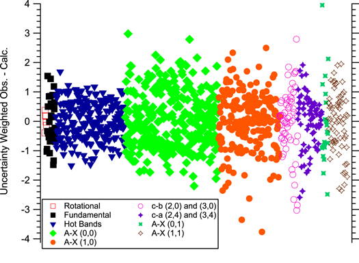
The weighted residuals for all the data sets show that the transitions are well distributed within ∼3σ, as can be seen in Figure 2. All the X state parameters are in good agreement with previous values (Rehfuss et al. 1992; Markus et al. 2016). It is difficult to directly compare the A state to the published parameters in Merer et al. (1975) and Rodgers et al. (2007) because the spin–orbit split levels were fit with separate origins for each spin component rather than using the spin–orbit parameters. Moreover, the definitions for the Λ-doubling parameters as defined here are not the same as those used by Merer et al. (1975). The value of the perturbation parameter, PLSe, is similar to Rodgers et al. (2007) and Merer et al. (1975), and this is the first reported distortion parameter for the perturbation term.
Figure 2. Residuals from the global fit. The ordinate is normalized by the uncertainty assigned to each data set, which effectively means the data is plotted against the standard deviation. Most of the the data are contained within 3σ indicating a good quality fit.
Download figure:
Standard image High-resolution image
The predissociation states were all fit simultaneously with the perturbation, and the molecular parameters, as reported in Table 4, are in reasonable agreement with those published by Rodgers et al. (2007), except in cases were additional higher-order distortion corrections were included in the fit. In those cases, the lower-order parameters were generally similar, but not in complete agreement. As compared to previous work, more transitions were fit together to determine the perturbation matrix element thereby taking advantage of more data to improve the accuracy of the value of the perturbation.
3.2. Astrophysical Implications
These molecular constants represent the first modern fitting of the A3Π–X3Σ− system. These new constants are particularly useful for rapid, easy simulations of spectra for both the optical and infrared using the program PGOPHER (Western 2017). Although PGOPHER can calculate the transition frequencies of for the submillimeter spectrum, because the hyperfine was not considered, it is preferable to use the values in CDMS (Endres et al. 2016) for calculating those spectral features.
The new constants for the X3Σ− state can be utilized in the search for infrared transitions. These spectral features are most likely important in shocked and highly ionized sources. Interference from telluric water absorption poses a challenge for ground-based observations. This work has also shown that the v = 5 − 4 vibrational band must be deleted from the list of known transitions as it may have been assigned in error by Rehfuss et al. (1992).
This work also is critically important for the analysis of optical spectra. There have been many examples of detections of OH+ in the near-UV since the first was done by Krełowski et al. (2010) (Gredel et al. 2011; Porras et al. 2014; Bhatt & Cami 2015; Zhao et al. 2015). Given the recent interest, it is important to revisit the uncertainties of the spectral features first measured by Merer et al. (1975).
In Merer et al. (1975), the precision of the fit is limited to only 0.09 cm−1, and the accuracy is about 0.02 cm−1. The accuracy of this work is equivalent to Stark et al. (1994) at 0.0005 cm−1, and it has an average precision of 0.025 cm−1. The precision of many of the higher signal-to-noise lines is substantially better. The analysis of de Almeida & Singh (1981) presented a list of the transitions expected to be detectable. Zhao et al. (2015) observed six transitions in translucent clouds. In many cases, this work represents a substantial improvement on the uncertainty of those lines, which are summarized in Table 6.
Table 6. A List of Astrophysically-relevant Transitions in Wavelength in Standard Air
| Transition | Merer et al.a (Å) | This Work (Å) |
|---|---|---|
| (0,0) qQ11(1) | 3587.923(15) | 3587.92650(16) |
| (0,0) rR11(0) | 3583.756(15) | 3583.75574(16) |
| (0,0) rR11(1) | 3579.471(15) | 3579.47011(15) |
| (0,0) qQ22(1) | 3577.134(15) | 3577.133(12)b |
| (0,0) rQ21(0) | 3572.648(15) | 3572.65187(33) |
| (0,0) rR22(1) | 3570.658(15) | 3570.6631(11) |
| (0,0) sR21(0) | 3566.445(15) | 3566.4458(11) |
| (0,0) rP31(0) | 3565.341(15) | 3565.34592(81) |
| (0,0) sQ31(0) | 3559.807(15) | 3559.8062(13) |
| (0,0) tR31(0) | 3553.329(15)c | 3552.325(12)b |
| (1,0) qQ11(1) | 3350.596(13) | 3350.5956(15) |
| (1,0) rR11(0) | 3346.960(13) | 3346.95559(74) |
| (1,0) rR11(1) | 3343.640(15) | 3343.6395(10) |
| (1,0) qQ22(1) | 3341.221(13) | 3341.223(11)b |
| (1,0) rQ21(0) | 3337.358(13) | 3337.3570(15) |
| (1,0) rR22(1) | 3335.957(13) | 3335.959(11) |
| (1,0) sR21(0) | 3332.177(13) | 3332.177(11)b |
| (1,0) rP31(0) | 3330.409(13) | 3330.409(11)b |
| (1,0) sQ31(0) | 3326.367(13) | 3326.369(11)b |
| (1,0) tR31(0) | 3319.971(13)c | 3319.967(11)b |
Notes. The values determined in this work are between 1 and 2 orders of magnitude more certain than the previous values recorded by Merer et al. (1975), although not all were observed. The non-observed transitions have been calculated with the new constants.
aData from Merer et al. (1975). bSimulated with new molecular constants. cSimulated with data from Merer et al. (1975) by Zhao et al. (2015).Download table as: ASCIITypeset image
One important note is that up until this point, the transition notation relied on the quantum number J, which is the total angular momentum (see especially Table 2 and Figure 1). Merer et al. (1975) and de Almeida & Singh (1981) used the quantum number N, which is the rotational angular momentum, in the transition labels. The relation between J and N is given by  , where
  is the electron spin. For this reason, the labels in Table 6 differ from those in Table 2 by 1 in the parenthesis.
The data in Table 6 are presented as wavelength in standard air using the updated index of refraction from Birch & Downs (1994) based on the work by Edlén (1966). The errors were propagated forward considering both the error in the index and the error in the wavenumber, and are directly compared to the original values by Merer et al. (1975), which were presented by de Almeida & Singh (1981) and Zhao et al. (2015). Although not all observations were reproduced, the ones that were all resulted in at least an order of magnitude of improvement. The average precision of the fit and the calibration are taken together to estimate the uncertainty in the simulated line positions. The largest discrepancy between the current work and that of Zhao et al. (2015) is the  transition, which was simulated in both cases. The error is ∼1 cm−1. Given the similarity with the decimal figures and the agreement between the two simulations for the
  transition, it is possible that the value reported in Zhao et al. (2015) is a typographical error. The most commonly observed transition is the feature at 3583.756 Å, and the new value is two orders of magnitude more certain. These values should be very useful in measuring Doppler shifts.
4. Conclusions
These molecular parameters are the best parameters for the calculating transition frequencies and energy levels that are currently published. The  Hamiltonian for a diatomic molecule using the program PGOPHER for a 3Π − 3Σ− transition is used to fit Kitt Peak FTS transitions in a hollow cathode that had not been analyzed previously. The interaction between the b1Σ+ state and the A3Π state has to be included. The inclusion of the available rotational, rovibrational data and predissociation laser spectroscopy spectra allowed for the completion of the most inclusive fit achieved to date.
The National Solar Observatory (NSO) is operated by the Association of Universities for Research in Astronomy, Inc. (AURA), under cooperative agreement with the National Science Foundation. The OH+ spectrum was recorded by J. Brault and R. Engleman, and were obtained from the NSO data archives. A. Wong assisted with SPFIT/SPCAT simulations. Support was provided by the NASA Laboratory Astrophysics program.