


Abstract
Spatio-temporal entropy (STE) analysis is used as an alternative mathematical tool to identify possible magnetic cloud (MC) candidates. We analyze Interplanetary Magnetic Field (IMF) data using a time interval of only 10 days. We select a convenient data interval of 2500 records moving forward by 200 record steps until the end of the time series. For every data segment, the STE is calculated at each step. During an MC event, the STE reaches values close to zero. This extremely low value of STE is due to MC structure features. However, not all of the magnetic components in MCs have STE values close to zero at the same time. For this reason, we create a standardization index (the so-called Interplanetary Entropy, IE, index). This index is a worthwhile effort to develop new tools to help diagnose ICME structures. The IE was calculated using a time window of one year (1999), and it has a success rate of 70% over other identifiers of MCs. The unsuccessful cases (30%) are caused by small and weak MCs. The results show that the IE methodology identified 9 of 13 MCs, and emitted nine false alarm cases. In 1999, a total of 788 windows of 2500 values existed, meaning that the percentage of false alarms was 1.14%, which can be considered a good result. In addition, four time windows, each of 10 days, are studied, where the IE method was effective in finding MC candidates. As a novel result, two new MCs are identified in these time windows.
Export citation and abstract BibTeX RIS
1. Introduction
A subset of Interplanetary Coronal Mass Ejections (ICMEs) has simple flux rope-like magnetic fields. These kinds of events, the so-called interplanetary magnetic clouds (MCs), have a magnetic field strength higher than the average Interplanetary Magnetic Field (IMF), a magnetic field direction that rotates smoothly through a large angle, and low proton temperature (Burlaga et al. 1981; Klein & Burlaga 1982; Gosling 1990). In many cases, their configurations could be described by a force-free model as a simple approximation useful in the interpretation of time series data (e.g., Lepping et al. 1990; Osherovich & Burlaga 1997; and references therein). Because MCs move faster than the surrounding solar wind (SW), plasmas and magnetic field typically accumulate in front of it, creating a preceding disturbed sheath.
The rapid decrease in the total pressure with solar distance is the main driver of the radial expansion of the flux rope (Démoulin & Dasso 2009). If the MC is moving at the same speed as the environment SW but still expanding, it will disturb both the solar wind ahead of and behind it, creating sheath-like structures (although they may not be bounded by a shock front). The signature of an MC is smooth field rotation, regardless of whether or not the upstream SW is disturbed. However, if an MC is moving slower than the surrounding SW (Klein & Burlaga 1982; Burlaga 1988; Zhang & Burlaga 1988; Ojeda et al. 2014b), then it is difficult to detect the sheath region, and consequently, to find the candidate MCs, when visual inspection of the data is performed. If the shock wave produced by the ICMEs is spatially greater than the MC, then sometimes a spacecraft can only detect the shock wave (Schwenn 2006).
Near  , MCs have a tube radius of
  , radius of curvature
  (Burlaga 1995), an average duration of
  , an average peak of the magnetic field strength of
  , and an average SW speed of
  (Klein & Burlaga 1982). Many authors (e.g., Zwickl et al. 1983; Richardson & Cane 1995) have noted that sometimes individual signatures may not be detected in all MCs, because they are not present and/or there are data gaps.
In order to find plasma beta values significantly lower than 1 to identify MCs, spacecraft measurements of magnetic field and plasma are required. Sometimes the temperature and density data on a spacecraft have many gaps during periods where the plasma instruments are saturated as a result of intense particle fluxes (for example, Bastille Day on the ACE spacecraft). If this condition occurs, it is impossible to calculate the plasma beta, but it is still possible to detect the MC using magnetometer data (e.g., Huttunen et al. 2005; Nieves-Chinchilla et al. 2005).
The SW plasma generates complex fluctuations in spacecraft-recorded signals, which can be investigated with techniques adopted from Nonlinear Dynamics Theory (Remya & Unnikrishnan 2010) but taking into account the physical processes related to MCs. To settle these difficulties mentioned above, we are proposing here a nonlinear technique as an auxiliary tool to identify MC candidates using only the available magnetic field data.
2. IMF Data Set
The Lagrangian point L1 is a gravitational and centrifugal force equilibrium point about 1.5 million km from the Earth and 148.5 million km from the Sun. It provides a very useful position for monitoring the SW before it reaches the Earth. At this position, plasma particles and magnetic fields detected by a satellite arrive at the magnetopause after about  . The Advance Composition Explorer (ACE) spacecraft has made such measurements while orbiting L1 since 1997 (Smith et al. 1998).
The Magnetic Field Experiment (MAG; Smith et al. 1998) and the Solar Wind Electron, Proton, and Alpha Monitor (SWEPAM; McComas et al. 1998) on board ACE provided the measurements used in this work. The IMF and solar wind plasma data used in this work correspond to events from two main lists of interplanetary phenomena. One is the MC identification by Huttunen et al. (2005), which has the event number, year, shock time (UT), MC start time (UT), and MC end time (UT) of each event. The other is a summary by Richardson & Cane (2010) of the ICME occurrences recorded in the SW that reached the Earth from 1996–2009. They gave a detailed list of such events based on in situ observations. The previous MC list was also used by Ojeda et al. (2013, 2014b, 2014a). All these papers are worthwhile efforts in developing new tools to help diagnose Interplanetary Coronal Mass Ejection (ICME) structures.
Ojeda et al. (2013) showed that time series with records from 2000 to 4000 points are the most adequate to calculate a stable Spatio-Temporal Entropy (STE) value (Kononov 2002). In an SW interval of 12 hr, with a time resolution of  , 2700 data points exist. Thus, in this work, we use data from the IMF GSM components with a time resolution of
  . Real-time ACE data have a resolution of 5 minutes, thus using this methodology for space weather alerts could be limited. In an MC interval of ∼12 hr with a 5 minute resolution, 144 data points exist. The STE calculation should only be used to study time series with 2000–4000 points, and in this case, the best results are obtained with the
  resolution.
3. Methodology
Here, we will apply the STE methodology in order to identify the MC-candidate regions in a semi-automatic way, without using MC regions identified by previous works. The MC-candidate regions must have STE values close to zero in MC regions, as obtained by the statistical work of Ojeda et al. (2013, technique validation). The STE is calculated for each time series of Bx, By, and Bz. We expect to find at least one IMF component inside an MC region with a close to zero STE value, as observed by Ojeda et al. (2013). In the following, we will define an Interplanetary Entropy (IE) index from the STE results. The IE index is implemented as an auxiliary tool to find MC regions using only IMF components, without previous MC region identification. This is done for the first time here. With the MC candidates in hand, we will define the MC boundaries using Minimum Variance Analysis (MVA).
3.1. Entropy Analyses
The concept of entropy is fundamental to the study of several branches of physics, such as statistical mechanics and thermodynamics (Kolmogorov 1958). Loosely interpreted, entropy is a thermodynamic quantity that describes or quantifies the amount of disorder in a physical system. Therefore, we can generalize this concept to characterize or quantify the amount of information stored in more general probability distributions of time series (Shannon & Weaver 1948; Boffetta et al. 2002).
Several methods for calculating entropy exist (e.g., Shannon & Weaver 1948; Kolmogorov 1958; Sinai 1959). The STE was developed only for the Shannon entropy, i.e., the Boltzmann–Gibbs entropic formula restated in the framework of information theory (Boffetta et al. 2002). The relationship between entropy and Lyapunov exponents in cellular automata was discussed by Boffetta et al. (2002). For cellular automata, a new method for calculating the entropy, called the spatial-temporal entropy density, was proposed. In their study, it was said that this entropy cannot be practically computed. It is necessary to fix L = constant (spatial size) to compute the quantity called temporal entropy.
However, in this paper, the calculation of STE will be performed using Eugene Kononov's Visual Recurrence Analysis (VRA) software (Kononov 2002). The VRA has been successfully used by several authors (e.g., Dasan et al. 2002; Hermann 2005; Marwan 2008; Crisan 2012; Alexa et al. 2015). In the VRA software, Eugene Kononov gives a qualitative explanation how the STE is computed: "To get some measure of how 'structured' the recurrence plot is, you can also calculate its STE. STE measures the image 'structureness' in both space and time domains. Essentially, it compares the global distribution of colors over the entire recurrence plot with the distribution of colors over each diagonal line of the recurrence plot. The higher the combined differences between the global distribution and the distributions over the individual diagonal lines, the more structured the image is. In physical terms, this quantity compares the distribution of distances between all pairs of vectors in the reconstructed state space with that of distances between different orbits evolving in time. The result is normalized and presented as a percentage of 'maximum' entropy (randomness). That is, 100% entropy means the absence of any structure whatsoever (uniform distribution of colors, pure randomness), while 0% entropy implies 'perfect' structure (distinct color patterns, perfect 'structureness' and predictability)."
The entropy proposed by Boffetta et al. (2002) and VRA has the same name, "STE," and both are based on the Shannon entropy. However, they are not the same method because one entropy is calculated over the cellular automata and the other over the recurrence plot.
The physical justification for using the STE method to study MCs was discussed by Ojeda et al. (2013). In the force-free model solution with constant alpha (Lundquist 1951; Burlaga 1988), the time series of the tangential component, BT, from the analytical solution is given by  , where
  is the sign providing the handedness of the field helicity, B0 is an estimate of the field at the axis of the cloud, R is the radial distance from the axis, and J1 is the Bessel function of order 1. Ojeda et al. (2013) found that the STE value of the tangential component BT is zero. The relevance of the previous result is that STE values of zero are found inside the MC region because of its magnetic structure. This fact is due to the well-organized structure of the magnetic field frozen inside the MC region. In many cases, as an approximation, part of the BT fit could be observed in one or two of the three IMF components. In any orthogonal reference system, e.g., GSE or GSM, the STE can be calculated from the three IMF components. Then, this peculiarity can be used to identify the existence of MCs or, in a more conservative approach, MC candidates. The comparison with other entropy methods in order to identify MC regions is not within the scope of this paper. Nonetheless, this topic was briefly discussed by Ojeda et al. (2013), without any deep investigation.
3.1.1. Interplanetary Entropy Index
Using the STE method, we analyzed IMF data using a time interval of 10 days, ensuring that a wide interval that contains the occurrence of at least one pre-identified MC will be used. As a criterion for IE index calculation, we select a convenient data interval of 2500 records moving forward by 200 record steps until the end of the time series. For every data segment, the STE is calculated at each step. It allows the analysis of the STE evolution along the series, with an adequate resolution defined by the chosen step. We select 2500 points because this interval represents an interval of  , and the MCs have a smooth magnetic field vector rotation on the order of 1 day, where the field reaches a peak and decreases (Burlaga 1988). With a temporal window size of
  and a resolution of
  , it is possible to cover the entire range of the trend in most MCs with time extension larger than
  . The STE calculation has stable values in time series with data points from 2000 to 4000 records (see Ojeda et al. (2013, Figure 2). Moreover, if this interval is shorter than 2500 points, then the STE value could be close to zero in places that are not cloud regions. Therefore, this methodology may not be applicable in identifying small and weak MCs. The STE values are calculated every
  (time resolution adopted, with 200 records) and represent ∼8% of the size of each temporal window. Thus, the variation of the STE values between two adjacent windows of
  must also be in the order of
  .
.

Figure 1. Scheme used to identify MCs.
Download figure:
Standard image High-resolution imageIn summary, higher STE value variation (close to 100%) indicates disorganization, i.e., no flux rope structure, while lower value variation (close to zero) indicates that organization has been reached, i.e., a flux rope-like structure.
Based on the MC magnetic structure, not all of the magnetic components are expected to have STE values close to zero simultaneously. We expect to find at least one component with entropy close to zero. However, this value should exist for two hours or longer. This is the reason for creating a standardized interplanetary entropy index (the so-called IE index). This index, joined with the STE, results for the three variables  , which are affected by the physical process, in an easily interpreted diagnosis. The index is the result of the multiplication of the STE values obtained from the calculation on each of the three variables, using a data set taken at the same time t, and normalized by 104. It is given by

This normalization is convenient for showing the IE index in the same scale as the STE, from 0% to 100%. The IE should be less than ≈1.5% (where zero is the best result) to consider the region an MC candidate. Therefore, the threshold chosen is ≈1.5%. We report the IE index as an approximate value.
3.2. Minimum Variance Analysis
The minimum variance analysis (MVA) is a traditional method of calculating the MC boundaries (Klein & Burlaga 1982; Bothmer & Schwenn 1998; Huttunen et al. 2005). For MCs with durations of 12 hr or less, Huttunen et al. (2005) performed MVA using 5 minute (WIND) or 4 minute (ACE) averaged data. The minimum variance analysis will look at matrix eigenvalue problems for the measured magnetic field data, where the three corresponding eigenvectors  of the matrix can be calculated. The cloud axis
  is calculated from the eigenvector components (Sonnerup & Scheible 1998). The axis
  can have any orientation over the ecliptic plane.
The coordinate system in which to calculate the MC axis angles  is as follows: the x-axis is the Earth–Sun line (in the Earth frame), the y-axis is in the ecliptic plane and perpendicular (in the east direction) to the Earth–Sun line, and the z-axis is normal to the ecliptic, toward the ecliptic north pole. Accordingly,
  and
and  are the poles of the magnetic field
  and the azimuthal
  angles, respectively. A flux-rope category (SEN-type) is often used to classify an MC where the magnetic field vector rotates from the south (S) at the leading edge and to the north (N) at the trailing edge, being eastward (E) at the axis. In order to classify MCs, eight flux rope categories are usually used (see Bothmer & Schwenn 1998; Huttunen et al. 2005, and references therein): for bipolar MCs (low inclination, i.e.,
  ) and flux-rope type, SWN, SEN, NES, and NWS; and for unipolar MCs (high inclination, i.e.,
  ) and flux-rope type, WNE, ESW, ENW, and WSE. Here, the properties of the MC flux-rope structure are studied. Therefore, we also use MVA to define the MC boundaries not identified by previous authors.
3.3. Identification of MC Occurrence
We use the STE and IE methods to identify the MC and/or MC candidates. If there is an MC or MC candidate, the boundaries are calculated using MVA. The step-by-step methodology scheme used to identify the MC occurrence is presented in Figure 1. Its description is divided into Part I and II as follows.
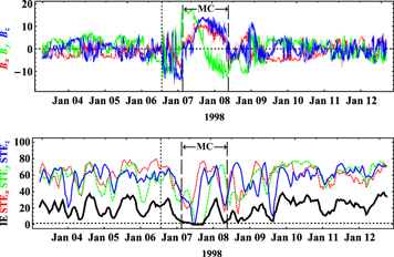
Figure 2. Values of the spatio-temporal entropy (STE) as a function of time for the time series of IMF  and the
  components in the SW. The thick curve represents the entropy index (IE) calculated over the analyzed period. The shock, start, and end times of the MC, given in Table 1, are represented by three vertical lines,
Download figure:
Standard image High-resolution imageIn Part I of the scheme, the IMF data (in any reference system) with the best time resolution are acquired. Then data in an arbitrary time interval are taken, using an interval large enough to contain a significant portion of an eventual MC. After that, records from the data taken within a convenient time length (called window) are selected in each displacement under a constant time step until the end of the data series. The STE value is then calculated in each window respectively for the 
 and Bz components, which allows the time evolution for the STE to be obtained. Finally, the IE values are calculated using Equation (1). When IE is close to zero
  for a period of time, then there is an MC-candidate region, and it can be examined in order to identify the MC boundaries.
In Part II of the scheme, after identifying the MC occurrence and its probable location, the evaluation of the MC boundaries can be done using the IMF data or, if available, by also using the SW plasma data, for more precise results. For the MC boundary analysis, MVA can be applied on the IMF data. A more complete analysis is done using plasma beta calculation resulting from the plasma data and IMF data together. The MC regions are characterized by a decrease in the plasma beta value, and here we use this characteristic to validate the MC candidates. In the end, both the identification and the characterization of MCs are done.
4. Results and Discussion
In this section, we will present the results of the MC candidate identification. In Part I, our positive and negative cases will be discussed, as well as the false alarms. In Part II, we will characterize two MC events not reported by previous authors.
4.1. Results: Part I
In order to test the proposed identification methodology and demonstrate its usefulness, three well-identified events by other authors are now used. Table 1 presents three MCs selected from the work of Huttunen et al. (2005). In Table 2, the SW intervals used to analyze these events are shown. An ICME (from Dal Lago et al. 2006) is also included to verify the quality of the method. This phenomenon is chosen to test the ability of the tool to distinguish MCs from other ICMEs.
Table 1. MC Events Identified by Huttunen et al. (2005)
| Year | Mon | Shock | Start | Stop | type |

|

|
|---|---|---|---|---|---|---|---|
| 1998 | Jan | 06, 13:19 | 07, 03:00 | 08, 09:00 | ENW | 21 | 52 |
| 1999 | Feb | 18, 02:08 | 18, 14:00 | 19, 11:00 | NWS | 96 | 06 |
| 2000 | Oct | 12, 21:36 | 13, 17:00 | 14, 13:00 | NES | 33 | −25 |
Note. Columns: year, month, shock time (UT), MC start time (UT), MC end time (UT), inferred flux-rope type, and direction of the MC axis ( ,
,  ).
).
Download table as: ASCIITypeset image
Table 2. Solar Wind Intervals Studied
| Year | Month | Start | Stop | Sist | Windows | Type |
|---|---|---|---|---|---|---|
| 1998 | Jan | 03, 00:00 | 12, 23:59 | GSM | 258 | MC |
| 1999 | Oct | 20, 00:00 | 25, 23:59 | GSM | 150 | no MC |
| 1999 | Feb | 14, 00:00 | 23, 23:59 | GSM | 258 | MC |
| 2000 | Oct | 08, 00:00 | 17, 23:59 | GSM | 258 | MC |
| 2010 | Apr | 01, 00:00 | 10, 23:59 | GSE | 258 | ?? |
Note. Columns: year, month, SW start time interval, SW stop time interval, coordinates system, total of 11.11 hour windows in the intervals, and type of event.
Download table as: ASCIITypeset image
4.1.1. Positive Cases
Based on the test case of the MC on 1998 January 6–8, (see Table 1), an SW data set of 10 days, from 1998 January 3–12 (see Table 2), is selected. The STE is calculated in a total of 256 time windows, each with 2500 records. In Figure 2, we show the STE values versus date for the time series of the IMF components for this interval. STE values for Bx, By, and Bz are plotted with a dotted line, dashed line, and continuous thin line, respectively. In addition, we investigate if ACE detected some other event during those 10 days.
Richardson & Cane (2010) reported two ICMEs in this interval: from January 7, 01:00, to January 8, 22:00, the event has an MC; while from 1998 January 9, 07:00, to January 10, 08:00, no event is classified as an MC. Thus, in Figure 2, we have one MC, one interplanetary disturbance not classified as an MC, and a quiet SW period. The MC was also reported by Huttunen et al. (2005), but with a different size.
In Figure 2 (both panels), the shock, start, and end of the MC are represented by three vertical lines, at the times listed in Table 1. In the top panel, components of the interplanetary magnetic field are plotted. In the bottom panel, the dashed horizontal line is the threshold of  . The previous line is plotted in other similar figures in this work where the IE is shown. The
  components have zero STE values
  only during the passage of the MC, approximately in its first half. The second minimum value of
  corresponds to the Bz component on January 9. On this date (January 9, 07:00–January 10, 08:00), Richardson & Cane (2010) detected one ICME. It is not classified as an MC. This result is very interesting, because in this interval of 10 days of SW data, only two magnetic components (
 ) have STE values of zero, and it is within the MC. Huttunen et al. (2005) first performed a visual inspection of the data to find the cloud candidates. This is always the first step in any work aimed at studying MCs. Although automatic ways of identification exist, the plasma data still need to be used in the usual tools (Lepping et al. 2005). Therefore, the calculation of the STE could be a very useful mathematical tool to help find MC candidates.
The thick curve in Figure 2 represents the IE calculated along the analyzed period. The IE value can only decrease close to zero  somewhere inside the MC. MCs have simple flux rope-like magnetic fields with enhanced strengths and which rotate slowly through a large angle. The time series of the IMF components show a trend toward more ordered dynamic behavior and a higher degree of correlation with its temporary neighbors (Ojeda et al. 2005, 2013). The aforementioned behavior is found only in the magnetic structures of the MCs or flux rope-like magnetic fields, a necessary condition for the threshold IE value.
4.1.2. Negative Cases
The IE methodology is required to validate that the STE is not zero for any other interplanetary disturbance, except for MCs. This is the reason why the term "negative case" is used here. Although it is not a true proof, this empirical test corroborates the results that have been obtained for a large number of SW data. This case, chosen to create a difficult situation for analysis because of its physical similarity with the MC, serves as an example of validation, or initial acceptance, of the method.
In Table 2, an SW data set of 6 days, from 1999 October 20–25, is indicated. The interface between the interplanetary ejecta and high-speed stream on 1999 October 22 is an excellent study case (Dal Lago et al. 2006). High-speed streams, originating in coronal holes, are often observed following ICMEs at 1 au (Klein & Burlaga 1982). Dal Lago et al. (2006) studied the 1999 October 17–22 solar-interplanetary event, which was associated with a very intense magnetic storm ( ).
).
Figure 3, bottom panel, shows the values of STE as a function of time for the time series of the IMF  components in the SW from 1999 October 20–25. In these SW data intervals, 150 time windows (each with 2500 records) were obtained. STE values of each of the three IMF components are calculated. Using Equation (1), the IE is calculated and plotted (thick curve) over the analyzed period in this figure.
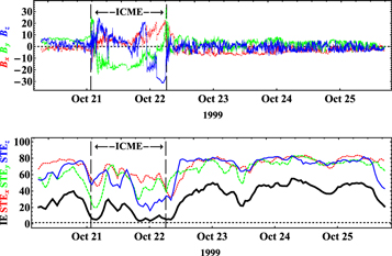
Figure 3. Values of STE as a function of time for the time series of the IMF  and
and  components in the SW. The thick curve represents the IE calculated over the analyzed period. The vertical lines represent the ICME reported by Dal Lago et al. (2006) from Oct 21, 01:34 UT to Oct 22, 06:15 UT.
Download figure:
Standard image High-resolution imageDal Lago et al. (2006) presented an analysis of pressure balance between the ICME observed on October 21–22 and the high-speed streams following it. Close to the Earth, at L1, an interplanetary shock was detected by the ACE magnetic field and plasma instruments on 1999 October 21, 01:34, shown in Figure 3 by the first vertical dotted line. The driver of this shock is an ICME, which can be distinguished from the normal SW by its intense magnetic field, of the order of  throughout most of October 21, and by its low plasma beta (∼0.1) (Dal Lago et al. 2006). The start of the ejecta was on October 21, 03:58. Toward the end of this ejecta, an increase of the magnetic field intensity was observed, starting on October 22, 02:30, reaching a peak value of
  (Dal Lago et al. 2006). At 06:15 UT on October 22 (the second vertical dotted line in Figure 3), the magnetic field dropped abruptly around
  . Dal Lago et al. (2006) defined this point as the end of the ICME. They were not sure whether or not this ICME has an MC according to the criteria of Burlaga et al. (1981), because the direction of the magnetic field does not rotate smoothly. Richardson & Cane (2010) also detected an ICME that was not classified as an MC, from 1999 October 21, 08:00, to October 22, 07:00.
It is clear that during the period of 1999 October 20–25, no event was identified as an MC. In Figure 3, the values of the STE are always different from zero, so the IE index is also different from zero. This result helps validate the use of IE in detecting MCs. The IE index methodology can differentiate when an ICME is not classified as an MC, because the IE index is only close to zero ( ) inside an MC. This capability is related to the correct diagnosis of the intrinsic magnetic field configuration existing in an MC, representing a very high organized plasma structure.
4.1.3. A Blind Test Case
With the idea of trying the method, we randomly selected one MC among the 80 MC events (73 MCs and 7 cloud candidates) identified by Huttunen et al. (2005). It is the second case in Table 1, identified as the MC event of 1999 February 18–19. Table 2 indicates the 10 day interval, 1999 February 14–23, of the collected SW data set to be analyzed. Considering a total of 256 time windows, the STE values are calculated. The result is shown in Figure 4, bottom panel. The STE reaches a value of zero for the Bx component. Thus, there is an IE index presenting a value of zero in the examined period.
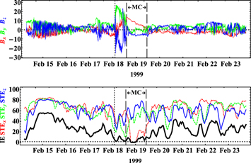
Figure 4. Plot of the IE as a function of time, 1999 February 14–23, but the three vertical lines correspond with the third event in Table 1. The format is the same as in Figure 2.
Download figure:
Standard image High-resolution imageRichardson & Cane (2010) detected an ICME that is not classified as an MC, from 1999 February 13, 19:00 to February 14, 15:00. Figure 4 shows the results of the calculation of the STE on 1999 February 14, 15:00, where the IE has a small, but non-zero, value. During 1999 February 18–21, the ACE spacecraft detected an ICME (that has an MC) (Richardson & Cane 2010). Inside the MC, which is delimited by the vertical lines in Figure 4,  only for one IMF component (in this case, for Bx). It generates an IE index with a value of zero only inside the MC region. Therefore, the IE index indeed shows the occurrence of one MC event in this data interval. So far, we often see MCs with STE values of zero only in one of the IMF components. However, the IE has always detected the existence of MCs through the threshold value. Thus, using the IE index, we can find the MC occurrence but not its boundaries (or time extension). The consistent results from other aleatory cases are not shown in this work.
4.1.4. How Successful is the IE Analysis versus Other Identifiers of MCs?
Thirty-three near-Earth ICMEs in 1999 have been chosen from the catalog of Richardson & Cane (2010, their Table 3). In the previous manuscript, a "2" in Column 15 indicates that the ICME includes an MC reported on the WIND MCs list (Wu et al. 2003) or by Huttunen et al. (2005). A "1" indicates that there is evidence of rotation in the magnetic field direction, but overall, the magnetic field characteristics do not meet those of an MC. Events with no MC-like magnetic field features are indicated by "0." Thirteen near-Earth ICME included MCs, of which seven are indicated with "1" and six with "2." In Table 3 from rows 1 to 3, the three previous cases are shown. Column 2 shows the total number of MCs. Column 3 shows the total number of MCs  in column 2 that were identified with the IE methodology, i.e., where the IE is less than 1.5%. A success rate of 100% is the best result. The successfulness of the IE index methodology is calculated using the equation (
 /Total) × 100%. The IE index analysis versus another identifier of MCs (Richardson & Cane 2010, Table 3) has an average successfulness of ≈70%. The unsuccessful cases (≈30%) are caused by small and weak MCs.
Table 3. Summary of Three Previous Studies That Identified MCs in 1999
| List of MCsa | Total | NIEb | Successfulnessc |
|---|---|---|---|
| 1 | 13 | 9 | 69.2% |
| 2 | 7 | 5 | 71.4% |
| 3 | 6 | 4 | 67.7% |
| 4 | 9 | 5 | 55.5% |
| 5 | 4 | 3 | 75.0% |
Notes. Successfulness of the IE methodology when compared with previous works.
aIn column 1: "1," Richardson & Cane (2010, Table 3); "2," Richardson & Cane (2010, Table 3) (events listed as "1" in the paper); "3," Richardson & Cane (2010, Table 3) (events listed as "2" in the paper); "4," Huttunen et al. (Table 2, 2005); "5," Wu et al. (/WIND list 2003). bMCs that have been identified by IE methodology, where the IE is less than 1.5%. c(NIE/Total) × 100%.Download table as: ASCIITypeset image
The same study explained in the above paragraph was performed with two other identifiers of MCs (see Huttunen et al. 2005, their Table 2, and Wu et al. 2003, /WIND list). In Table 3, the results are shown in the last two columns. The low successfulness (55.5%) with Huttunen et al. (2005) has an explanation. The IE methodology was unsuccessful in four events: one event was identified as a cloud candidate (cl) with a time extension of eight hours; two events were classified as MCs, however, on that date ICMEs were not reported; and the last MC was also identified by Wu et al. (2003, /WIND list, event 42 (September 21) with poor quality (3) and with a time extension of seven hours.
4.1.5. False Alarm Cases
Furthermore, we saw false alarm cases. False alarm cases are grouped into three categories: (1) non-MC ICMEs according to the catalog of Richardson & Cane (2010, Table 3) (20 of these cases were identified); (2) stream interaction regions (SIRs) according to the catalog of Jian et al. (2006, p. 367–371), where 36 SIRs were identified; (3) other cases (non-MC ICMEs and non-SIRs). In Table 4, the previous categories are shown. In the first category, 15% of false alarms are reported. This is important and can save time, e.g., when a specialist wants to identify new MCs in a large data period. These three cases could be MC-ICME; however, they are not studied in this work.
Table 4. Summary of Events That Are Not MCs Reported in 1999 and False Alarm Cases in the IE Analysis
| False Alarm Cases | Total | NIEa | Pb |
|---|---|---|---|
| Non-MC ICMEs | 20c | 3 | 15% |
| SIRs | 36d | 1 | 2.8% |
| Other cases (non-ICMEs and non-SIRs) | ⋯ | 5 | ⋯ |
Notes.
aNumber of false alarm cases, i.e., where .
bPercent of false alarm cases
.
bPercent of false alarm cases  /Total) × 100%).
cAdapted from Richardson & Cane (2010, Table 3), from 33 ICMEs: 13 were MCs-ICMEs and 20 were non-MC ICMEs.
dJian et al. (2006, p. 367–371).
/Total) × 100%).
cAdapted from Richardson & Cane (2010, Table 3), from 33 ICMEs: 13 were MCs-ICMEs and 20 were non-MC ICMEs.
dJian et al. (2006, p. 367–371).
Download table as: ASCIITypeset image
In the second category, there is only one false positive case. In summary, the IE methodology is not useful to identify SIRs. Finally, five cases are in the third category. These cases are interesting because disturbances in the IMF can be observed. In addition, we are left with two open questions. What really are these events? Why do they have low IE values, similar to an MC? We think that these cases could be flux ropes. However, further study should be done to investigate the above cases.
In summary, the IE methodology identified 9 from 13 MCs, and nine false alarm cases are emitted. In a year (1999), a total of 788 windows of 2500 values exist, which means that the percent of false alarms was 1.14%, which is a good result. However, we prefer to propose it as a preliminary result because one year is considered poor statistics to accept the result as a robust identifier of MCs. Despite the difficulties, we can conclude that the IE methodology is useful for studying MCs, and in the next section, the IE methodology is used to identify two MCs.
4.2. Results: Part II
After tests on efficiency, the methodology is applied to study some SW cases and also to demonstrate its utility. Some novelties are discovered. Table 1, last column, presents one MC identified by Huttunen et al. (2005). In Table 2, the last two columns, the SW data intervals used for the analysis are shown. All of them are intervals with 10 days of SW data.
4.2.1. Analysis of the 2000 October 12–14 Event
Using the same procedure applied to the earlier cases, a study is done on the period including the 2000 October 12–14 event (presented in Table 1). The extended 10 day interval is shown in Table 2. In Figure 5 (bottom panel), the STE values for each component as a function of time are plotted with different line types. The thick black curve represents the IE calculated along the analyzed period. The MC around October 14 is plotted with three vertical dashed lines (the shock and cloud boundaries). The properties of this cloud are described by Huttunen et al. (2005). During the passage of this MC, the  components have
  approximately in its first half, and the IE identifies this MC
  . As expected, the STE method was once again demonstrated to be useful and capable of producing valid results.
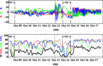
Figure 5. IE plotted as a function of time, 2000 October 8–17, but the three vertical lines correspond with the event in Table 1. The format is the same as in Figure 2.
Download figure:
Standard image High-resolution imageHowever, on October 8, the  components have STE values of almost zero (
 and
and  ), with
  . On this date, the presence of an ICME was not reported, but a small magnetic structure where the field had a smooth variation is noticeable.
To identify MC boundaries, a combination of analyses of plasma data with the MVA method is usually applied. The data was measured by ACE from 2000 October 7 to 9, with a 1 hr time resolution. Figure 6 is composed of six panels: (top panels) magnetic field strength and polar (Blat) angles of the magnetic field vector in the GSE coordinate system; (middle panels) azimuthal (Blong) angle and plasma beta; (bottom panels) maximum and minimum variance planes, respectively. The plasma beta minimum value was  on October 7 at 23:00 UT. We used the magnetic field rotation confined to one plane and the plane of the maximum variance
  to find the boundaries of the cloud; the dates are written in Table 5. In all panels of Figure 6, the first vertical line indicates the shock and the other two vertical lines indicate the MC interval. The MVA method gives the eigenvalue ratio
  , the angle between the first and the last magnetic field vectors
  , the orientation of the axis
  , the direction of minimum variance
  , and eigenvalues
 ![$[{\lambda }_{1},{\lambda }_{2},{\lambda }_{3}]=[124.6,41.8,0.9]$](https://content.cld.iop.org/journals/0004-637X/837/2/156/revision1/apjaa6034ieqn72.gif) . This MC has a flux rope-type SEN as can be seen in Figure 6, right top panel and left middle panel, respectively. The observed angular variation of the magnetic field is left-handed. An MC event has been characterized. The STE method demonstrates not only its usefulness, but also its capability to produce new results (or, at least, interesting cases for studies). However, a question remains: how is it possible to identify a cloud in a region without ICMEs? Therefore, we think that this event is caused by the partial-halo CME on 2000 October 4, 06:26:05, which leaves the Sun with a linear speed of 237 km s−1 (see the CME catalog, http://cdaw.gsfc.nasa.gov/CME_list/).
. This MC has a flux rope-type SEN as can be seen in Figure 6, right top panel and left middle panel, respectively. The observed angular variation of the magnetic field is left-handed. An MC event has been characterized. The STE method demonstrates not only its usefulness, but also its capability to produce new results (or, at least, interesting cases for studies). However, a question remains: how is it possible to identify a cloud in a region without ICMEs? Therefore, we think that this event is caused by the partial-halo CME on 2000 October 4, 06:26:05, which leaves the Sun with a linear speed of 237 km s−1 (see the CME catalog, http://cdaw.gsfc.nasa.gov/CME_list/).
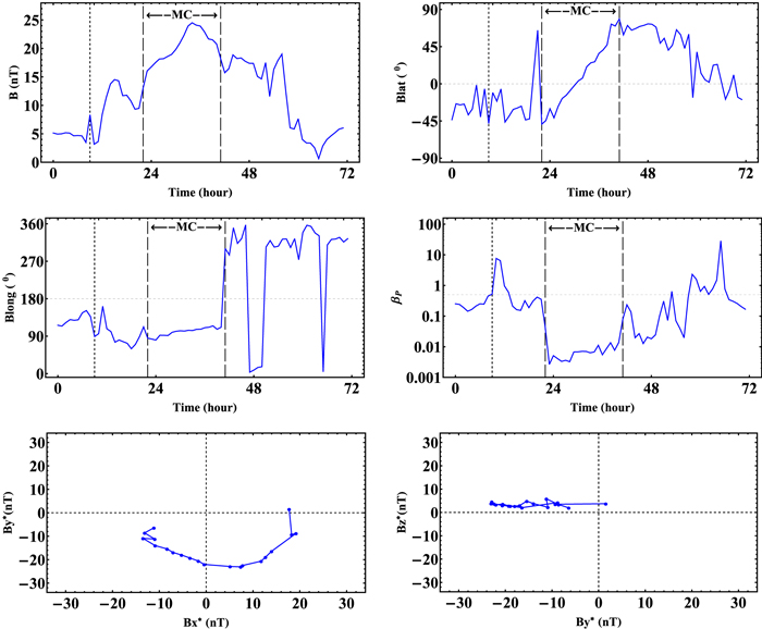
Figure 6. Bipolar MC observed by ACE on 2000 October 7–9 and identified in this work. The figure is composed of six panels, from (a) to (f): magnetic field strength, polar (Blat) and azimuthal (Blong) angles of the magnetic field vector in the GSE coordinate system, proton plasma beta, rotation of the magnetic field vector in the plane of maximum variance, and rotation of the magnetic field vector in the plane of minimum variance.
Download figure:
Standard image High-resolution imageTable 5. Magnetic Cloud from 2000 October 7–8
| Year | Shock | MC, start | MC, stop |
|---|---|---|---|
| 2000 | Oct 7 09:00 | Oct 7 22:00 | Oct 8 17:00 |
Download table as: ASCIITypeset image
4.2.2. Analysis of 2010 April 5–6 Event
On 2010 April 3, the Sun launched a cloud of material, known as a coronal mass ejection (CME), in a direction that reached the Earth. This CME was very fast, with a speed of at least  . The bulk of the CME passed south of the Earth, but a piece of it hit the Earth's magnetosphere on April 5, causing a geomagnetic storm (
 on April 6 at
  UT).
UT).
The ACE Magnetic Field Experiment data in level 2 (verified) were not available in 2010 April when the data were processed (2010 April–May). It was only possible to obtain such data for 16 s average IMF in RTN or GSE coordinates via anonymous ftp, from Caltech.7 For this reason, in Figure 7 (bottom panel), the STE values are calculated using data in GSE coordinates. This is not a problem, because the choice of the coordinate system, i.e, GSE, GSM, or RTN, does not affect the methodology for this study.
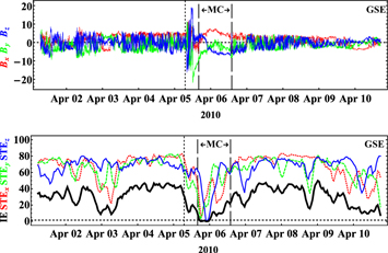
Figure 7. IE plotted as a function of time, for 2010 April 1–11. The shock and MC boundaries are shown with three vertical lines. Those dates were identified in this work. The format is the same as in Figure 2. The thick curve represents the IE calculated over the analyzed period. The MC is identified.
Download figure:
Standard image High-resolution imageIn Figure 7 (bottom panel), we find minimum values of  in the Bz component on April 5 at 21:33:20 and 22:26:40 UT. The Bx and By components had STE values less than 10% on April 5 from 18:00:00 to 18:53:20 UT, respectively. Then, the IE has a minimum value of less than 1.5% on day 5, from 18:00:00 to 23:20:00 UT. Thus the IE detects a structure with characteristics of a MC candidate.
We think that an MC exists inside of these ICMEs. The methodology implemented in this work identifies a region characteristic of an MC in the magnetic field data. Using the earlier treatments, the boundaries found for the MC candidate is delimited in the data shown in Figure 8.

Figure 8. SW windows observed by ACE from 2010 April 1 to 10, in the GSE coordinate system and with a  time resolution.
Download figure:
Standard image High-resolution image
In Figure 8, the data are measured by ACE from 2010 April 1–11, with a  time resolution. The figure is composed of six panels: (top panels) magnetic field strength and polar (Blat) angles of the magnetic field vector in the GSE coordinate system, (middle panels) azimuthal angle (Blong) and plasma beta, (bottom panels) planes of maximum and minimum variance, respectively. On 2010 April 5, at 07:00 UT, the proton density was
  , proton temperature
  , ratio of alphas/protons = 7 × 10⁻², proton speed
  , magnetic field magnitude
  , and plasma beta
  . One hour later, some parameters had changed:
  ,
,  , alphas/protons = 1.7 × 10⁻²,
  ,
,  , and
, and  . It is easy to identify a shock because the velocity, density, and magnetic field magnitude increase abruptly, and we believe that it is related to the arrival of an event at ACE. Eight hours after the time of the shock, at
  UT, the plasma beta decreases to
  , and it is the start of the MC.
The plasma beta minimum value was  on April 6 at 12:00 UT. We used the magnetic field rotation confined to one plane, the maximum variance plane
  , to find the boundaries of the MC. The dates are shown in Table 6. The minimum variance plane
  has a problem, because the plot is not in
  (there is an offset), and we report this MC to be of medium quality in the identification. Thus, in all panels of Figure 8, the first vertical line indicates the shock and the other two vertical lines show the MC interval. The MVA method gives the eigenvalue ratio
  , the angle between the first and the last magnetic field vectors
  , the orientation of the axis
  , the direction of minimum variance
  , and eigenvalues
 ![$[{\lambda }_{1},{\lambda }_{2},{\lambda }_{3}]=[16.8,3.6,0.2]$](https://content.cld.iop.org/journals/0004-637X/837/2/156/revision1/apjaa6034ieqn99.gif) . This MC has the flux rope-type NWS, as can be seen in Figure 8, right top panel and left middle panel, respectively. The observed angular variation of the magnetic field is left-handed. With the proposed methodology, we were able to identify a new MC.
. This MC has the flux rope-type NWS, as can be seen in Figure 8, right top panel and left middle panel, respectively. The observed angular variation of the magnetic field is left-handed. With the proposed methodology, we were able to identify a new MC.
Table 6. Magnetic Cloud from 2010 April 5–6
| Year | Shock | MC, start | MC, stop |
|---|---|---|---|
| 2010 | Apr 5 07:00 | Apr 5 16:00 | Apr 6 14:00 |
Download table as: ASCIITypeset image
By calculating the STE of the magnetic structures, evaluated by an IE index, the methodology proposed here allows MC candidates to be identified, as well as revealing some of them that present interesting features for further studies. The use of computational techniques to identify MC candidates seems better than performing an exhausting visual inspection of the data set to find the MC candidates, as done in other studies. Although there are other identification methodologies, another advantage of the IE index methodology is that it deals only with the IMF data. Finally, we should emphasize that this methodology is only an auxiliary identification tool, to be added to the others.
5. Conclusions
The STE, and consequently the IE index, is implemented as an auxiliary tool to find MC regions using only IMF components and without using MC regions previously identified by other authors. The results of this paper include detecting MCs compiled in earlier works (Wu et al. 2003; Huttunen et al. 2005; Richardson & Cane 2010), as well as new MC candidates with interesting features deserving further investigations. In addition, the use of MVA analysis is also possible, using only the IMF data to delimit the MC boundaries.
The IE index was tested in a whole year (1999) in order to validate it. Despite simplicity of the method, the proposed approach shows effective analysis with little computational effort. One advantage of this numerical tool is that it can indeed help the specialist, who only uses visual inspection, by allowing a pre-selection of MC candidate cases.
The IE index was proposed here for the first time. To build the methodology, we calculated the STE, as a function of time, for IMF components using magnetic records within time windows corresponding approximately to 11.11 hr, physical parameters representative of MC events, displaced consecutively by a proper time step until the end of the data series. The STE reached values extremely close to zero for at least one of the IMF components during the MC event, due to MC structure features. Not all of the magnetic components in MCs had STE values close to zero at the same time. The IE index was very convenient because it allowed the STE results of the three IMF components to be joined into one estimate parameter, which allowed for easy interpretation. Therefore, if the IE index was close to zero  , it indicated the occurrence of an MC candidate, and its probable time location.
In order to be clear about the STE approach, some comments can be made on the method's primary features. We did not use the techniques of bi-directional streaming of supra-thermal SW electrons (BDE) along magnetic field lines to find the MC candidates (Bame et al. 1981; Gosling 1990). On one hand, BDEs are also present in ICMEs without the MC structure, and we should also use plasma data to build it. On the other hand, calculation of the IE does not use plasma data. This is an advantage of the IE index over the BDE technique, added to the fact that IMF data usually have few or short gaps and a better time resolution. The capability of the strategy is to show how a mathematical tool like the STE, which allows an easy computational technique, can simply and quickly identify the occurrence of a flux rope-like structure associated with the cloud at about  .
.
In summary, the IE analysis versus other identifiers of MCs had a success rate of 70%. The unsuccessful cases (30%) were caused by small and weak MCs. The IE methodology identified 9 of 13 MCs, and nine false alarm cases were emitted. In 1999, a total of 788 windows of 2500 values existed, meaning that the percent of false alarms was 1.14%, which can be considered a good result. Also, two new MCs were identified here on 2000 October 7–8 and 2010 April 5–6.
This work was supported by grants from CNPq (grants 483226/2011-4, 307511/2010-3, 301441/2013-8, 165873/2015-9, 306038/2015-3, and 312246/2013-7, 306828/2010-3), FAPESP (grants 2012/072812-2 and 2007/07723-7), and CAPES (grants 1236-83/2012 and 86/2010-29). A.O.-G. thanks CAPES and CNPq (grant 141549/2010-6) for his PhD scholarship and CNPq (grant 150595/2013-1) for his postdoctoral research support. V.K. wishes to thank her financial support within the Programa Nacional de Pós-Doutorado (PNPD—CAPES) We are grateful to V.E. Menconni for helpful computational assistance. Acknowledgments are due to Eugene Kononov, author of the Visual Recurrence Analysis software. In addition, the authors would like to thank the ACE science team members for the data sets used in this work. Also, A.O.G. thanks the INPE for the financial support and facilities.