Observable Signatures of Energy Release in Braided Coronal Loops

Observations of the Sun's atmosphere reveal coronal loops with lengths from 1000 Mm down to 1 Mm (Peter et al. 2013), and widths down to at least 0.1 Mm (Brooks et al. 2013; Aschwanden & Peter 2017). The internal structure of these loops remains a controversial topic—in particular whether they are composed of discrete strands, and the length scales and heat distributions of such strands. A review of observations and modeling of coronal loops is presented in Reale (2014). The tangling of magnetic field lines within the corona has long been proposed as a mechanism for heating the Sun's atmosphere to the observed multi-million degree temperatures (Parker 1972, 1988). However, there remains a debate over whether the observations are consistent with such field line braiding; indeed most observed loops exhibit a "well combed" appearance, with this being used to argue against the braiding mechanism. On the other hand, López Fuentes et al. (2006) argued that the approximately constant cross section of observed loops (Klimchuk 2000) can be explained by a tangling of loop strands below observable scales inhibiting expansion toward the loop top. By contrast, considerations of cross-field particle diffusion and observations of coronal rain dynamics have been used to argue against significant field line tangling in loops (Galloway et al. 2006; Antolin & Rouppe van der Voort 2012; in the latter case, at least on perpendicular scales above a few hundred km). Schrijver (2007) claimed that the absence of strand tangling in loop observations could be explained by a continuous reconnection process that prevents the tangling occurring, although as pointed out by Berger & Asgari-Targhi (2009), the absence of a tangled appearance does not preclude internal braiding of loop strands. Recently, Cirtain et al. (2013) reported the first direct evidence of braided loops in the solar atmosphere. In this paper we move to clarify the interpretation of the observations by determining synthetic emission patterns during energy release events in braided magnetic fields.

Before proceeding further we address the following question: why should we expect energy release in a braided magnetic field? Pontin & Hornig (2015) demonstrated that any force-free equilibrium for such a tangled magnetic field must contain thin current layers, with these current layers being thinner for increasing levels of tangling (see Pontin et al. 2016 for a discussion of how this tangling can be quantified). Specifically, the current layer thickness in the equilibrium is shown to scale with the smallest scales present in the field line mapping (defined, for example, by the full width at half maximum of any quantity that is projected along field lines onto a loop cross section). Therefore, as the coronal field is driven toward a progressively more tangled configuration, it will inevitably reach a state containing current layers that are sufficiently thin/intense to undergo reconnection on a fast (Alfvénic) timescale—even at coronal plasma parameters. This critical level of field line braiding is difficult to determine precisely due to the absence of a well developed theory for reconnection onset in three dimensions (see the discussion of Pontin & Hornig 2015). However, we expect that the coronal field should exist in a statistically steady state of marginal stability around this critical braiding level. This marginally stable state is then maintained through a competition between the photospheric driving that acts to increase the field line tangling and magnetic reconnection that simplifies the topology (cf. Galsgaard & Nordlund 1996). In this paper we determine the observational signatures that arise following the onset of energy release in a braided magnetic field.

The High Resolution Coronal Imager (Hi-C; Cirtain et al. 2013; Kobayashi et al. 2014) provided unprecedented high-quality coronal images and first detected two locations of braided coronal structures in an active region corona. Hi-C images, with a spatial resolution of about 150 km and a cadence of 5 s, were obtained using a narrow passband filter centered at 193 Å, which is emitted by Fe xii at about 1.5 MK (Cirtain et al. 2013). Thalmann et al. (2014) constructed a nonlinear force-free field and verified the presence of these braided structures, also finding that these braided loops were rather low lying compared with other coronal loops (see also Del Zanna 2013). The large braided loop, numbered "1" in Cirtain et al. (2013), was very dynamic and produced more than 10 subflares—in many cases triggered externally due to interaction with an erupting coronal loop from underneath—over 4 hours of Solar Dynamics Observatory/Atmospheric Imaging Assembly (Lemen et al. 2012) observations (Tiwari et al. 2014).

A careful inspection of the Hi-C movie (see Figure 1) reveals emission patterns indicative of braiding on multiple spatial scales (perpendicular to the global loop geometry). In particular, there are several local/smaller braided structures apparent within the large magnetic braided structure "1" discovered by Cirtain et al. (2013). In Figure 1 we indicate by white arrows two locations of such apparent local braids out of several noticed in the movie (see the animation linked to Figure 1). The large braided magnetic structure can be rather easily identified in the normal intensity images (see the red arrow in Figure 1, and the same location in the animation). Additionally, we have created unsharp masked images that allow clearer identification of small-scale apparently twisted and/or braided structures within the loop (compare the locations indicated by arrows in the panels of Figure 1 and the associated animation). Unsharp masking is a technique that enhances the image quality by increasing the sharpness and contrast of images, thus allowing features to be identified more clearly. This technique has been successfully applied for solar image processing in the past (Aschwanden 2010; Cirtain et al. 2013; Alpert et al. 2016).

At several locations during the animation it appears as if two strands cross each other, co-spatial with local intensity enhancements. Thus the braiding of strands and heating of plasma seem to clearly be linked, at least in some cases. The standard interpretation is that such bright crossing loops correspond to energy release associated locally with two stressed bundles of magnetic field lines. We investigate the link between the emissions and magnetic field structure further in Section 6. The figure and the movie provide evidence for the braiding of strands and for localized heating at numerous locations (independently of whether a localized braid is found) throughout the large-scale braided region. This observed tangling on multiple scales is consistent with the behavior in the simulations presented in Section 4.

As discussed previously, the coronal magnetic field is expected to exist in a state of marginal stability in which field line braiding by boundary motions is balanced by reconnection events that act to untangle the field. However, accessing this state in computer simulations is impossible, since the small numerically accessible magnetic Reynolds number means that reconnection sets in too early (i.e., before the field has become sufficiently tangled that one would expect reconnection at coronal parameters). We therefore (artificially) separate the field line tangling process and the energy release process by supposing that the field has already been braided by the boundary motions. Specifically, we take a magnetic field with braided field lines as our initial condition, and analyze the turbulent relaxation that follows the onset of reconnection.

Here we consider two different magnetic braids. One unknown factor is the degree of braiding that one expects in the corona before the energy release process sets in. The degree of braiding that we consider is on the conservative side, being rather low compared to the predicted braiding required for reconnection onset in the corona (Pontin & Hornig 2015). The explicit expressions for the magnetic fields, referred to as Braid 1 and Braid 2, are presented in the Appendix, and some representative magnetic field lines are plotted in Figure 2. Both magnetic fields are based on the same "protocol" of alternating (in z) twists of opposite signs (offset in x). Braid 1 is the same field as considered in a series of works in recent years (Wilmot-Smith et al. 2009a, 2010; Pontin et al. 2011), and is characterized by an efficient tangling of field lines throughout the central portion of the domain ($\sqrt{{x}^{2}+{y}^{2}}\lesssim 2.5$)—see Figure 2(a). Braid 2 is a similar field in which the twist profile in each of the twist regions is modified, with a further six smaller twist regions also added. This produces three coherent flux tubes embedded within the tangled region—see the red, blue and black flux tubes in Figure 2(b). More quantitative insight can be gained into the structure of our two model braids by examining the mapping of field lines between the upper and lower boundaries ($z=\pm 24$) in each case. In a highly braided field, adjacent field lines may diverge rapidly from one another, leading to strong gradients in the field line mapping. This may be quantified by calculating the squashing factor Q associated with the mapping. By introducing

$$\begin{eqnarray}&&N=\sqrt{{\left(\displaystyle \frac{\partial X}{\partial x}\right)}^{2}+{\left(\displaystyle \frac{\partial X}{\partial y}\right)}^{2}+{\left(\displaystyle \frac{\partial Y}{\partial x}\right)}^{2}+{\left(\displaystyle \frac{\partial Y}{\partial y}\right)}^{2}},\end{eqnarray} \tag{ 1 }$$

the squashing factor is defined as

$$\begin{eqnarray}&&Q=\displaystyle \frac{{N}^{2}}{| {B}_{z}(x,y)/{B}_{Z}(X,Y)| },\end{eqnarray} \tag{ 2 }$$

where x and y are field line footpoints on $z=-24$, and X and Y are the corresponding footpoint locations on $z=Z=24$ (Titov et al. 2002; Pariat & Démoulin 2012). Now, as discussed by Wilmot-Smith et al. (2009b), the efficient tangling of field lines renders the distribution of Q to be a foliation of thin layers (individually referred to as quasi-separatrix layers) filling the braided region. This can be seen for Braid 1 in Figure 3(a), where we observe a relatively homogeneous tangling (i.e., thin layers of high Q are evenly distributed and spaced throughout $\sqrt{{x}^{2}+{y}^{2}}\lesssim 2.5$). By contrast, the coherent flux tubes present in Braid 2 can be seen—see Figure 3(e)—as "holes" in the foliation of Q layers, since within the flux tubes we have regular concentric flux surfaces without any significant stretching within the mapping.

Zoom In Zoom Out Reset image size

Zoom In Zoom Out Reset image size

Each of these magnetic fields is first ideally relaxed toward a force-free equilibrium using a magnetofrictional ideal relaxation scheme that exactly preserves the topology (Craig & Sneyd 1986) in order to smooth out the twist regions and extract some of the excess energy associated with this artificial initial condition. We then transfer the magnetic field to an MHD code using the method described in Wilmot-Smith et al. (2010). The code employed is the STAGGER code (Galsgaard & Nordlund 1997), which solves the standard induction, momentum, and continuity equations for single-fluid MHD, together with the following equation for the thermal energy $e=p/(\gamma -1)$, with p being the plasma pressure,

$$\begin{eqnarray}\displaystyle \frac{\partial e}{\partial t} & = & -{\rm{\nabla }}\cdot (e{\boldsymbol{v}})-(\gamma -1)e{\rm{\nabla }}\cdot {\boldsymbol{v}}+{H}_{v}+{H}_{J}\\ & & -{{\rm{\nabla }}}_{\parallel }\cdot ({\kappa }_{\parallel }{{\rm{\nabla }}}_{\parallel }T)-{{Fn}}_{e}{n}_{h}P(T),\end{eqnarray} \tag{ 3 }$$

where ${\boldsymbol{v}}$ is the plasma velocity; $\gamma =5/3$ is the ratio of specific heats; H_v and H_J are the viscous and Joule heating, respectively; ${\kappa }_{\parallel }=1.8\times {10}^{-10}({T}^{5/2}/\mathrm{ln}\,{\rm{\Lambda }}){\rm{W}}\,{{\rm{m}}}^{-1}\,{{\rm{K}}}^{-1}$ (Spitzer 1962); and for P(T) we use the function given by Klimchuk et al. (2008). F is a scaling parameter that we use to prevent the entire simulation domain from cooling too quickly—which is required since we do not continually resupply the plasma with energy through boundary driving. Rather, we consider a relaxation process with ${\boldsymbol{B}}$ line-tied and ${\boldsymbol{v}}=0$ on all boundaries (and the boundary values for e and the density ρ are then updated by locally solving the energy and continuity equations, respectively). We set F = 0.1 throughout. The equations include hyper-resistivity and hyper-viscosity terms that maximize the magnetic and fluid Reynolds numbers, and are solved over a uniformly spaced grid of ${360}^{2}\times 240$ points.

Dimensions in the simulations are chosen to match approximately with the Hi-C observations presented in Section 2 (though note that we do not claim to reproduce this particular event). We take a computational domain that is 12 Mm × 8 Mm × 48 Mm in size, centered at the origin, with the braided portion of the loop approximating a cylinder of length 48 Mm and diameter 2.5 Mm. The magnetic field strength is set by taking ${B}_{0}=100$ G. The initial state comprises a uniform plasma of density 2 × 10⁻¹¹ kg m⁻³, $T=7\times {10}^{5}$ K, meaning that in the initial state, $\beta \approx 0.013$. The simulation is run until t = 380 s.

Pontin et al. (2011) showed that, following the onset of reconnection in a braided magnetic field (whose free magnetic energy is initially concentrated at large scales), a turbulent cascade ensues, characterized by an array of both temporally and spatially localized current sheets. To quantify this we plot in Figure 4 the power spectrum of $| {{\boldsymbol{B}}}_{{xy}}{| }^{2}$, since the energy cascade takes place primarily perpendicular to the dominant field component along the loop, B_z (obtained by first performing an FFT in xy and then averaging over z). We note that at t = 0 the magnetic energy is predominantly at large scales. (One should take care not to confuse the scales of ${\boldsymbol{B}}$, which at t = 0 are large, with those exhibited by the field line mapping (Figure 3), which at t = 0 are small—this is a characteristic feature of magnetic braids.) The bump on the curve at high k_xy is an artefact of the interpolation method used to create the initial condition, and it quickly disappears. We observe during the simulation a transfer of energy to progressively smaller scales as the turbulent cascade develops. As shown in Figure 4, a spectrum with approximately constant gradient is then maintained between $t\approx 40\,{\rm{s}}$ and $t\approx 120\,{\rm{s}}$. We emphasize that the development of a turbulent field in the loop occurs self-consistently, being a natural consequence of the global field line complexity in the braided field. We note that due to the finite difference approach employed and moderate resolution, the inertial range is not clear to identify—however, as shown in Pontin et al. (2016), the inertial range extends as we reduce η (which here would correspond to an increased resolution). This generation of a turbulent cascade in the loop is consistent with previous theoretical studies addressing loop heating (e.g., Rappazzo & Velli 2011; Reale 2014; Velli et al. 2015; Dahlburg et al. 2016, and references therein) and with some of the latest loop observations (De Moortel et al. 2014), as well as being compatible with at least one interpretation of observed line broadening (e.g., Asgari-Targhi et al. 2014; Reale 2014, and references therein).

Zoom In Zoom Out Reset image size

The net result of the turbulent relaxation is that the field becomes less tangled, achieved through multiple small-scale reconnection events within the loop (and we emphasize that the boundaries are held fixed throughout). This reduction in the field line tangling can be observed by examining the evolution of the squashing factor Q in the domain, as shown in Figure 3. Clearly evident is a significant simplification of the field line mapping by the end of the simulation (seen as a reduction in the average of Q over field lines, indicating on average weaker divergence of neighboring field lines). This simplification begins, broadly speaking, once the turbulence begins to decay at $t\approx 100\,{\rm{s}}$. The relaxation (and associated untangling that is facilitated by many reconnections within the loop) finally yields a nonlinear force-free field—approximate due to the finite gas pressure—of much simpler topology than the initial braid (see Yeates et al. 2015, for a discussion of what determines the structure of this final state). The evolution of Braid 1 during the MHD simulations we perform is very similar to that described in Pontin et al. (2011). The only differences between the simulations are the inclusion of thermal conduction and radiative losses in the energy equation—which do not materially affect the magnetic field evolution due to the low plasma-β—and the use of hyper-resistivity rather than uniform resistivity, meaning that the current distribution is even more fragmented during the relaxation.

The resistive relaxation of Braid 2 follows the same qualitative behaviour as Braid 1: initial current layer formation is followed by the development and subsequent decay of a turbulent cascade, during which the field unbraids itself through many localized reconnection events. One primary difference, however, is that the presence of the coherent flux tubes in Braid 2 means that the current sheets that form during the relaxation are not homogeneously distributed throughout the loop as in the relaxation of Braid 1, but form preferentially on the surfaces of the coherent flux tubes (in addition to more "randomly" throughout the rest of the loop). As a result, there are certain flux bundles that are heated preferentially during the relaxation, which will be important when we come to consider the emission signatures. After $t\approx 50\,{\rm{s}}$, the coherent flux tubes are destroyed by the reconnection; see the significant shrinkage in the "holes" in the Q distribution that correspond to these coherent flux tubes between Figures 3(e) and (f). The turbulent relaxation again leads eventually toward a smooth nonlinear force-free equilibrium.

Synthetic emission patterns, integrated along various lines of sight, are obtained for the simulations using the FoMo package (Antolin & van Doorsselaere 2013; Van Doorsselaere et al. 2016) that has previously been used to forward model coronal loops supporting various wave modes (e.g., Antolin et al. 2014; Yuan et al. 2015). Line-integrated emission signatures are calculated for Fe xii (193 Å, $\sim 1.5\times {10}^{6}$ K) and Fe xv (284 Å, $\sim 2\times {10}^{6}$ K) lines by making use of CHIANTI v7 (Landi et al. 2013), and in particular the coronal abundances of Schmelz et al. (2012). The emission patterns do not change significantly if other coronal abundances are used—for example, using the abundances of Feldman (1992), who takes a higher iron abundance, leads to brighter emission though the same spatial distribution.

Emission patterns calculated for the Braid 1 simulation are plotted in Figure 5. The peak temperature attained during the simulation is $1.9\times {10}^{6}$ K. The heating occurs in numerous strands during the simulation, consistent with the fact that multiple thin current layers are formed. (Note that here we use "strand" to refer simply to a heated magnetic flux bundle; there is no significant density or $| {\boldsymbol{B}}|$ structuring across our loop due to the simplified plasma treatment.) We observe in the figure no obvious crossing of strands or braided appearance, although the heating seen as intense brightenings remains localized along more or less elongated strands. Toward the end of the simulation, the entire loop reaches a relatively homogeneous temperature, the heat being deposited relatively uniformly over the loop cross section. It is worth noting that the viewing angle can significantly affect the visual properties of the loop (Figure 5(b) and associated animation)—in particular for a line of sight (LOS) parallel to the x-axis, the loop gives the appearance of having a coherent twist, while the heating seems to be localized along longer strands. We note similarities to the emission patterns found by Botha et al. (2011), who studied a coherently twisted, kink-unstable loop, demonstrating that extreme care must be exercised in inferring twist or braiding from emission patterns. A further item of interest to note is that the spatial emission patterns are relatively unaffected if one "switches off" the conduction and radiation terms in the simulation—see the animation associated with Figure 5(a), although in that case the emission is more intense due to the absence of cooling and conduction. This indicates that in simulations with uniformly high plasma-β throughout the domain, qualitative emissions patterns can be approximated without the high computational expense of including these terms.

The Fe xii emission during the relaxation of Braid 2 is shown in Figures 6(a)–(d). Note that the 2Mm of the domain at either end of the loop is excluded from the plots, because strong heating occurs there at intermediate times in the simulations fuelled by a density evacuation. This is a well-known pitfall in MHD simulations of employing boundaries closed to mass flow—in reality we would expect evaporation to fill these cavities and thus reduce the extreme temperatures. (This artificial heating partially contaminates the footpoint regions in Figure 6(d).) What is evident from the emission patterns in the loop body for Braid 2 is a much clearer heating of many particular strands, and crossings of these strands, in contrast to Braid 1. This is because, as discussed previously, currents tend to focus on the surfaces of the coherent flux tube structures, which thus provide preferential locations for heat deposition. For Braid 2, the maximum temperature attained is also higher—since more heat is deposited on selected flux bundles (and therefore less on others)—reaching $5.6\times {10}^{6}$ K. Thus significant emission can also be observed in Fe xv, as shown in Figures 6(e)–(h). In this higher temperature line we naturally see fewer strands, and thus the braiding of the strands is less clear, unless one refers also to the Fe xii emission. By the end of the loop relaxation (Figure 6(d)), the entire loop reaches a homogeneous temperature, as for Braid 1, though with the heating spread over a broader radius. This is to a large extent though an artefact of the selected emission line—the loop is homogeneously heated at the end of the Braid 1 simulation, but much of the plasma has cooled below the temperature of the selected line.

In order to investigate what inferences we can draw from the LOS-integrated emissions, we have analyzed the relation between the observed bright strands and the magnetic field line structure. One typical interpretation is that bright crossing strands correspond to a "local braid," assumed to be a site of energy release. We would like to determine whether this is a valid conclusion based on the simulation results. We have analyzed a number of strand crossings at different times during both simulations. For clarity, here we describe an illustrative case taken from the Braid 2 simulation at t = 61 s.

Figure 7 shows the case of a bright "V-shape" of apparently crossing strands identified close to the loop center (between approximately z = 0 and z = 4), circled in frame (a), which is a close-up of Figures 6(b), (f). We note that on the outside of the Fe xii V-shape is a less pronounced, broader V-shape in the Fe xv emission. In frame (b) we show a 3D rendering of the Fe xii emission along the same LOS as in (a), and identify a number of features that appear to be co-spatial with the V-shaped structure (marked by red arrows). Field lines are plotted from the cores of these intensity enhancements (magenta, yellow, white, cyan field lines). The first thing that we note is that while the alignment of the magnetic field lines and the emission strands is generally good, it is not always perfect. In general we find that strands on the periphery of the braided tube (where reconnection events are infrequent) show almost perfect alignment, while those near the tube center (in this case particularly the yellow field lines in the figure) exhibit a finite angle between the field lines and emission strands. We hypothesize that this is due to the continuous reconnection of field lines in many small current layers in the center of the tube, leading to a situation in which field line connectivity changes cannot be neglected on the timescales of the motion of conduction fronts parallel to the field lines.

Zoom In Zoom Out Reset image size

Now, we would like to know whether the bright crossing strands correspond to local braids (i.e., energy release events). It turns out that the right leg of the "V" in the emission is formed by one fairly well defined strand in 3D space, corresponding to the magenta field lines. The alternative viewpoint in Figure 7(c) shows that the left half of the "V" consists of three separate strands of emissions at different depths in the field of view. While one of these (yellow field lines) is relatively close to the magenta field lines at the apparent point of crossing, the other two (white, cyan field lines) are at far separated locations. We find this to be fairly typical. In particular, at early times (e.g., t = 45 s, Figures 6(a), (e)) when there are fewer individual strands, bright crossing features are found to correspond in most cases to flux tubes that cross rather close to one another. However, at later times (e.g., $t\in [60\,{\rm{s}},80\,{\rm{s}}]$ when there are more strands and more crossings) it is much more likely that apparent crossing strands do not ever come close to one another, indicating that their crossing is simply an artefact of the direction of projection.

We now analyze in more detail the field structure in the vicinity of two adjacent crossing strands, to determine whether the local structure is as expected in the typical picture of energy release in braided fields. The model of Parker (1972) involves energy release at tangential discontinuities of ${\boldsymbol{B}}$ in the ideal limit. The finite resistivity of the simulation means that we would expect instead a rapid rotation of the field vector across current sheets, and the question is whether the crossing strands in the domain are related to such structures. In Figures 7(d), (e) we show in detail the emission patterns, current density, and field lines in the vicinity of the identified adjacent crossing strands (yellow and magenta field lines). While these strands are associated with locally tight bundles of field lines, we observe in the figure a rapid divergence of the field lines (green) between these two bundles, indicating a local rotation of the field vector. This is consistent with the presence of a current concentration (purple shading) between the two strands. We note further that the strands are actually located relatively far out on the flanks of this current layer: the plasma close to the current layer is actually emitting in Fe xv (and in the core of the current layer appears to be even hotter). Plasma associated with these inner regions is at least partly responsible for the "V" observed in the Fe xv LOS-integrated emission, but the legs of this "V" appear much broader probably due to the LOS along which they are viewed.

We have performed similar analyses to those described here at various times during the relaxation of Braid 1. We find many cases of crossings of adjacent bundles of field lines like those depicted in Figures 7(d), (e), without observing any clearly braided strands in the emission (see Figure 5). This indicates that the absence of clearly observed crossing strands in the LOS-integrated emission does not preclude a complex field line tangling in the loop.

This discussion leads to the conclusion that extreme care must be taken in interpreting strand crossings (or their absence) within observed coronal loops:

• 1.  
  The presence of bright crossing strands does not necessarily imply the local presence of a current sheet (energy release event)—the strands may be well-separated along the LOS.
• 2.  
  Observed strands need not match one-to-one with magnetic flux tubes, depending on the relative rates of field line connectivity change and thermal conduction.
• 3.  
  The appearance of any local energy release region is highly wavelength-dependent—depending on whether one views plasma from near the core of the current sheet or in the "inflow" (pre-reconnecttion) or "outflow" (post-reconnection) regions, very different strand configurations are observed.
• 4.  
  There may be a natural geometrical effect that hides much of the field line braiding from us in emissions: the highest intensities in LOS-integrated emissions will be obtained when the LOS is parallel to the long axis of the current sheet. However, from this angle there is no shear between field lines. With an LOS perpendicular to this direction, one observes crossing field lines, but the emission is more diffuse due to the geometry of the heated region of plasma (see the broad "V" shape in the Fe xv emission noted earlier in this section).
• 5.  
  One thing that can certainly be concluded is that the presence of numerous observed crossing strands indicates a globally complex tangling (or braiding) of the magnetic field. However, the absence of observed crossing strands does not imply that no field line tangling is present.

Our study of the emission signatures of energy release in braided coronal loops leads to the following principal conclusions:

• 1.  
  Energy release and heating in braided fields may or may not give a clear visual "braided" appearance to the loop.
• 2.  
  If the field line tangling in the loop is very efficient and the turbulence associated with the energy release is subsequently relatively homogeneous (across the loop), then we expect a uniformly heated loop without visible "strands," as in Braid 1. This may be the most common scenario on the Sun, where we expect the presence of continual photospheric driving and the much higher magnetic Reynolds number to lead to a more fully developed turbulence in the loop than obtained here in our simulations.
• 3.  
  If, in contrast to the above, the loop contains more structure (such as coherent flux tubes as in Braid 2, or perhaps separatrices as envisaged by, e.g., Priest et al. 2002), then we have demonstrated that we can expect enhanced heating on certain strands with less heating on others. This then leads to a braided appearance, as in Braid 2 that is consistent with the braided structures identified in the Hi-C observations in Section 2 and by Cirtain et al. (2013).
• 4.  
  We have identified in the Hi-C observations tangling of heated strands on a range of different perpendicular length scales—there appear to exist "sub-braids" within the larger scale braided loop. This is consistent with the behaviour in the simulations, as is clearly evident for example in Figures 6(b), (c). In general one would expect tangling on a range of scales within a given coronal loop, determined by the hierarchy of photospheric velocity scales that created the tangling. In the observations there are numerous local brightenings not apparently associated with crossing strands. There are a number of factors that influence the signatures of local energy release, and as such these brightenings may well also be associated with local "magnetic braids" (i.e., crossing bundles of magnetic field lines), in spite of the absence of crossing strands in the emission.
• 5.  
  As per the issues highlighted at the end of the previous section, care must be taken in drawing conclusions regarding observed crossing of bright features in loops. The existence of bright crossing strands does not necessarily imply local energy release. The presence of numerous crossing strands does, however, indicate a global complex tangling (or braiding) of the magnetic field in the loop.

The number and thickness of observable strands in any braided coronal loop undergoing heating will be dependent on a number of factors, in addition to the structure of the field as discussed previously. As shown by Pontin et al. (2011), the number of current sheets that forms during the braid relaxation depends on the magnetic Reynolds number of the simulation—and as such this also controls the distribution of energy deposition on strands. Furthermore, the geometry of the current sheets that form—planar or curved—should affect how many strands are visible. These factors and our simplified geometry can explain to some extent the differences between the observed and modeled braids. For example, the braided structure "1" in Cirtain et al. (2013) is described as having a "pinched" region (red arrow in Figure 1), and its net twist is found to increase with time (Cirtain et al. 2013; Thalmann et al. 2014), neither of which are the case in our simulation. Despite these differences, it is encouraging to note that the Fe xii emission intensities are comparable to those observed by Hi-C, perhaps indicating that the free energy (degree of field line tangling) we considered is not too unrealistic. One further shortcoming of the present simulations is the reduced radiative losses employed, meaning that heated strands take longer to cool than in reality. A future study will consider the use of a parameterized heating term and full radiative losses, to address timescale questions more accurately. In particular, the relationship between the timescales for field line tangling, relaxation (energy deposition), and cooling will be crucial to further explore signatures of field line braiding. In the future a more complete treatment of the loop plasma, including the full thermodynamics as well as effects of, for example, atmospheric stratification and partial ionization, should be pursued.

D.P. acknowledges financial support from the UK's STFC (grants ST/K000993, ST/N000714). S.K.T.'s research was supported by an appointment to the NASA Postdoctoral Program at NASA MSFC, administered by USRA under contract with NASA. Hi-C: MSFC/NASA led the Hi-C mission and partners include the SAO in Cambridge, Massachusetts; Palo Alto, California; UCLan in the United Kingdom; and LPIRAS in Moscow. Support by a research grant (VKR023406) from VILLUM FONDEN is acknowledged. The authors are grateful for discussions with P. Antolin, T. Van Doorsselaere, R. Moore. Visualizations in Figure 7 were made using the package VAPOR www.vapor.ucar.edu.

The two magnetic field expressions used to initialize the simulations are given for Braid 1 by

$$\begin{eqnarray}{\boldsymbol{B}} & = & {B}_{0}\left(1{{\boldsymbol{e}}}_{z}+\displaystyle \sum _{i=1}^{6}\kappa {(-1)}^{i}\right.\exp \left(-\displaystyle \frac{{(x-{x}_{i})}^{2}+{y}^{2}}{2}\right.\\ & & -\left.\displaystyle \frac{{(z-{z}_{i})}^{2}}{4}\right)\times \,(-y\,{{\boldsymbol{e}}}_{x}+(x-{x}_{i}){{\boldsymbol{e}}}_{y})),\end{eqnarray} \tag{ 4 }$$

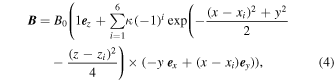
and for Braid 2 by

$$\begin{eqnarray}{\boldsymbol{B}} & = & {B}_{0}\left(1{{\boldsymbol{e}}}_{z}-\displaystyle \sum _{i=1}^{6}\displaystyle \frac{2\kappa {(-1)}^{i}}{\sqrt{\pi }\,\mathrm{erf}(2)}\exp (-2{({(x+2{x}_{i})}^{2}+{y}^{2})}^{2}\right.-{(z-{z}_{i})}^{2}/4)\times \,(-y\,{{\boldsymbol{e}}}_{x}+\,(x+2{x}_{i}){{\boldsymbol{e}}}_{y})\\ & & \left.\,+\,\left\{\begin{array}{cc}\displaystyle \sum _{i=1}^{6}0.506{(-1)}^{i}\kappa \sqrt{\pi }\exp \left(-\displaystyle \frac{{(z-{z}_{i})}^{2}}{4}\right){\left(1-{\left(\displaystyle \frac{{r}_{i}}{2.5}\right)}^{6}\right)}^{4}\times (-y\,{{\boldsymbol{e}}}_{x}+(x-{x}_{i}){{\boldsymbol{e}}}_{y})\,\,\,\, & {r}_{i}\leqslant 2.5\\ 0 & \mathrm{otherwise}\end{array}\right.\right).\end{eqnarray} \tag{ 5 }$$

where $\kappa =1$, ${{r}_{i}}^{2}={(x-{x}_{i})}^{2}\,+\,{y}^{2}$, ${x}_{i}={(-1)}^{i+1}$, and ${z}_{1..6}\,=\{-20,-12,-4,4,12,20\}$.