


Abstract
We present a promising new technique, the g-distribution method, for measuring the inclination angle (i), the innermost stable circular orbit (ISCO), and the spin of a supermassive black hole. The g-distribution method uses measurements of the energy shifts in the relativistic iron line emitted by the accretion disk of a supermassive black hole due to microlensing by stars in a foreground galaxy relative to the g-distribution shifts predicted from microlensing caustic calculations. We apply the method to the gravitationally lensed quasars RX J1131–1231 (zs = 0.658, zl = 0.295), QJ 0158–4325 (zs = 1.294, zl = 0.317), and SDSS 1004+4112 (zs = 1.734, zl = 0.68). For RX J1131−1231, our initial results indicate that rISCO ≲ 8.5 gravitational radii (rg) and i ≳ 55° (99% confidence level). We detect two shifted Fe lines in several observations, as predicted in our numerical simulations of caustic crossings. The current ΔE distribution of RX J1131–1231 is sparsely sampled, but further X-ray monitoring of RX J1131–1231 and other lensed quasars will provide improved constraints on the inclination angles, ISCO radii, and spins of the black holes of distant quasars.
Export citation and abstract BibTeX RIS
1. Introduction
One technique for measuring the innermost stable circular orbit (ISCO) and spin parameter a ( , where J is the angular momentum) of active galactic nuclei (AGNs) relies on modeling the relativistically blurred Fe Kα fluorescence lines originating from the inner parts of the disk (e.g., Fabian et al. 1989; Laor 1991; Reynolds & Nowak 2003). This relativistic iron line method has be applied to about 20 relatively bright, nearby Seyferts where the line is detectable with a high signal-to-noise ratio (S/N; Reynolds 2014 and Vasudevan et al. 2016). The sample sizes are starting to become large enough where the distribution of the spin parameter can be calculated and compared to simulated ones such as those presented in Volonteri et al. (2013). Even then, the Fe Kα line in most Seyferts is typically very weak, and constraining the spin and accretion disk parameters of Seyferts requires considerable observing time on XMM-Newton and Chandra. Moreover, the accuracy of the relativistic Fe line method for constraining the spin of a black hole from the broadened red wing of the Fe line profile is also questioned (e.g., Miller et al. 2009; Sim et al. 2012). We note, however, that independent measurements of the size of the corona from microlensing and reverberation mapping indicate that the X-ray source is compact, consistent with the lamppost model assumed in the relativistic Fe iron line method. Additional support for the relativistic Fe line method is provided by 3–50 keV observations with NuSTAR, such as the recent observations of Mrk 335 that indicate a spin parameter of >0.9 at 3σ confidence. The high-energy NuSTAR spectra can help to constrain the reflection component and better distinguish between models (Parker et al. 2014). Most of the measured spin parameters in Seyfert galaxies are found to be ≳0.9 (e.g., Reynolds 2014 and references therein). This may be the result of a selection bias in flux-limited samples (Vasudevan et al. 2016). Specifically, high-spin black holes are more luminous and hence brighter for a given accretion rate, and therefore will simply be more highly represented in flux-limited surveys. Recent observations and simulations (Fabian 2014; Keck et al. 2015; Vasudevan et al. 2016) also suggest that rapidly spinning black holes will tend to have stronger reflected relative to direct X-ray emission, making it easier to measure the spin parameter in these objects.
The relativistic iron line method has been applied to the gravitationally lensed quasars RX J1131–1231 (Reis et al. 2014) and Q2237+0305 (Reynolds et al. 2014), as well as to a stacked spectrum of 27 lensed 1.0 < z < 4.5 quasars observed with Chandra (Walton et al. 2015). Specifically, the relativistic disk reflection features were fit with standard relativistic Fe Kα models to infer inclination angles and spin parameters of  and
and  for RX J1131–1231 (Reis et al. 2014) and i ≲ 11
 5 and
5 and  for Q2237+0305 (Reynolds et al. 2014).
These studies have not, however, correctly accounted for the effects of gravitational microlensing. Gravitational microlensing is a well-studied phenomenon in lensed quasars (e.g., see the review by Wambsganss 2006, and references therein) where stars near the lensed images produce time-variable magnification of source components whose amplitude depends on the location and size of the emission region. In particular, in our analysis of the X-ray spectra of lensed quasars (Chartas et al. 2016), we have frequently observed structural changes in the Fe Kα emission, indicating that the line emission is being differentially microlensed. Thus, applying the relativistic Fe Kα line method to stacked spectra of lensed quasars, without accurately accounting for microlensing, is likely to lead to unreliable and unrealistic results.
In Section 2 we present the X-ray observations and analyses of the Chandra observations of RX J1131–1231, QJ 0158–4325, and SDSS 1004+4112. In Section 3 we discuss our recently developed technique based on microlensing to provide a robust constraint on the inclination angle, the location of the ISCO, and the spin parameter, and we present an analytic estimate of the fractional energy shifts g = Eobs/Erest and numerical simulations of microlensing events. In Section 4 we present our results from modeling the observed distribution of g and the distribution of the measured energy separations of shifted Fe Kα lines in cases where two shifted lines are detected in an individual spectrum. Finally, in Section 5 we rule out several alternative scenarios to explain the shifted iron lines and present a summary of our conclusions. Throughout this paper we adopt a flat Λ cosmology with H0 = 67 km s−1 Mpc−1, ΩΛ = 0.69, and ΩM = 0.31 (Planck Collaboration et al. 2016).
2. X-Ray Observation and Data Analysis
We have performed multiwavelength monitoring of several gravitationally lensed quasars (e.g., see Table 1 of Chartas et al. 2016 and references within) with the main scientific goal of measuring the emission structure near the black holes in the optical, UV, and X-ray bands in order to test accretion disk models. The X-ray monitoring observations were performed with the Chandra X-ray Observatory (hereafter Chandra). The optical observations (B, R, and I bands) were made with the SMARTS Consortium 1.3 m telescope in Chile. The UV observations were performed with the Hubble Space Telescope. In this paper we focus on constraining the inclination angles, ISCO radii, and spin parameters of quasars RX J1131–1231, QJ 0158–4325, and SDSS 1004+4112 using the Chandra observations of these objects.
RX J1131–1231 (hereafter RXJ1131) was observed with the Advanced CCD Imaging Spectrometer (ACIS; Garmire et al. 2003) on board the Chandra X-ray Observatory 38 times between 2004 April 12 and 2014 July 12. Results from the analysis of observations 1–6 of RXJ1131 were presented in Chartas et al. (2009) and Dai et al. (2010), and those for observations 7–29 are in Chartas et al. (2012). Results from the analysis of a subset of these observations have also been presented in Blackburne et al. (2006), Kochanek et al. (2007), and Pooley et al. (2012). Here we describe the data analysis for the remaining nine observations, but we will use the results from all 38 observations in our microlensing analysis. QJ 0158–4325 (hereafter QJ0158) was observed with ACIS 12 times between 2010 November 6 and 2015 June 10, and SDSS 1004+4112 (hereafter SDSS1004) was observed with ACIS 10 times between 2005 January 1 and 2014 June 2. Results from the analysis of the first six observations of QJ0158 and the first five observations of SDSS1004 were presented in Chen et al. (2012).
We reanalyzed all of the Chandra observations of RXJ1131, QJ0158, and SDSS1004 using the software CIAO 4.8 with CALDB version 4.7.2, provided by the Chandra X-ray Center (CXC). Logs of the observations for each object in our study that include observation dates, observation identification numbers, exposure times, ACIS frame times, and the observed 0.2–10 keV counts are presented in Tables 1–3. The properties of our sample are presented in Table 4. We used standard CXC threads to screen the data for status, grade, and time intervals of acceptable aspect solution and background levels.
Table 1. Log of Observations of Quasar RX J1131–1231
| Chandra | Exposure | ||||||||
|---|---|---|---|---|---|---|---|---|---|
| Epoch | Observation | JDa | Observation | Time | tfb | NAc | NBc | NCc | NDc |
| Date | (days) | ID | (ks) | (s) | counts | counts | counts | counts | |
| 1 | 2004 Apr 12 | 3108 | 4814 | 10.0 | 3.14 |

|

|

|

|
| 2 | 2006 Mar 10 | 3805 | 6913 | 4.9 | 0.741 |

|

|

|

|
| 3 | 2006 Mar 15 | 3810 | 6912 | 4.4 | 0.741 |

|

|

|

|
| 4 | 2006 Apr 12 | 3838 | 6914 | 4.9 | 0.741 |

|

|

|

|
| 5 | 2006 Nov 10 | 4050 | 6915 | 4.8 | 0.741 |

|

|

|

|
| 6 | 2006 Nov 13 | 4053 | 6916 | 4.8 | 0.741 |

|

|

|

|
| 7 | 2006 Dec 17 | 4087 | 7786 | 4.88 | 0.841 |

|

|
417
|

|
| 8 | 2007 Jan 01 | 4102 | 7785 | 4.70 | 0.441 |

|

|

|

|
| 9 | 2007 Feb 13 | 4145 | 7787 | 4.71 | 0.441 |

|

|

|

|
| 10 | 2007 Feb 18 | 4150 | 7788 | 4.43 | 0.441 |

|

|

|

|
| 11 | 2007 Apr 16 | 4207 | 7789 | 4.71 | 0.441 |

|

|

|

|
| 12 | 2007 Apr 25 | 4216 | 7790 | 4.70 | 0.441 |

|

|

|

|
| 13 | 2007 Jun 04 | 4256 | 7791 | 4.66 | 0.441 |

|

|

|

|
| 14 | 2007 Jun 11 | 4263 | 7792 | 4.68 | 0.441 |

|

|

|

|
| 15 | 2007 Jul 24 | 4306 | 7793 | 4.67 | 0.441 |

|

|

|

|
| 16 | 2007 Jul 30 | 4312 | 7794 | 4.67 | 0.441 |

|

|

|

|
| 17 | 2008 Mar 16 | 4542 | 9180 | 14.32 | 0.741 |

|

|
1337
|

|
| 18 | 2008 Apr 13 | 4570 | 9181 | 14.35 | 0.741 |

|

|
1453
|

|
| 19 | 2008 Apr 23 | 4580 | 9237 | 14.31 | 0.741 |

|

|
1279
|

|
| 20 | 2008 Jun 01 | 4619 | 9238 | 14.24 | 0.741 |

|

|

|

|
| 21 | 2008 Jul 05 | 4653 | 9239 | 14.28 | 0.741 |

|

|
1001
|

|
| 22 | 2008 Nov 11 | 4782 | 9240 | 14.30 | 0.741 |

|

|

|

|
| 23 | 2009 Nov 28 | 5164 | 11540 | 27.52 | 0.741 | 36024
|

|
2420
|
3827
|
| 24 | 2010 Feb 09 | 5237 | 11541 | 25.62 | 0.741 |

|

|
2059
|
2437
|
| 25 | 2010 Apr 17 | 5304 | 11542 | 25.67 | 0.741 |

|

|
1962
|
2813
|
| 26 | 2010 Jun 25 | 5373 | 11543 | 24.62 | 0.741 | 18521
|

|
1522
|
1487
|
| 27 | 2010 Nov 11 | 5512 | 11544 | 25.56 | 0.741 |

|

|
1821
|
1730
|
| 28 | 2011 Jan 21 | 5583 | 11545 | 24.62 | 0.741 |

|

|
1008
|

|
| 29 | 2011 Feb 25 | 5618 | 12833 | 13.61 | 0.441 |

|

|

|

|
| 30 | 2011 Nov 9 | 5875 | 12834 | 13.61 | 0.441 |

|

|

|

|
| 31 | 2012 Apr 11 | 6229 | 13962 | 13.67 | 0.441 |

|

|

|

|
| 32 | 2012 Nov 7 | 6239 | 13963 | 14.57 | 0.441 |

|

|

|

|
| 33 | 2012 Nov 18 | 6250 | 14507 | 9.13 | 0.441 |

|

|

|

|
| 34 | 2012 Dec 12 | 6274 | 14508 | 9.13 | 0.441 |

|

|

|

|
| 35 | 2013 Nov 30 | 6627 | 14509 | 9.13 | 0.441 |

|

|

|

|
| 36 | 2014 Jan 3 | 6661 | 14510 | 8.75 | 0.441 |

|

|

|

|
| 37 | 2014 Jun 13 | 6822 | 14511 | 9.13 | 0.441 |

|

|

|

|
| 38 | 2014 Jul 7 | 6851 | 14512 | 10.04 | 0.441 |

|

|

|

|
Notes.
aJulian Date–2450000. bACIS frame time. cBackground-subtracted source counts for events with energies in the 0.2–10 keV band. The counts for images A and B of RX J1131–1231 are corrected for pileup. Images C and D are not affected by pileup.Download table as: ASCIITypeset image
Table 2. Log of Observations of Quasar Q J0158−4325
| Chandra | Exposure | ||||||||
|---|---|---|---|---|---|---|---|---|---|
| Epoch | Observation | JDa | Observation | Time | tfb |
 c
c
|
 c
c
|
 c
c
|
 c
c
|
| Date | (days) | ID | (ks) | (s) | counts | counts | counts | counts | |
| 1 | 2009 Nov 06 | 5142 | 11556 | 5.03 | 1.74 | 103 ± 10 | 43 ± 7 | 35 ± 6 | 11 ± 3 |
| 2 | 2010 Jan 12 | 5209 | 11557 | 5.02 | 1.74 | 125 ± 11 | 61 ± 8 | 35 ± 6 | 19 ± 4 |
| 3 | 2010 Mar 10 | 5266 | 11558 | 5.04 | 1.74 | 146 ± 12 | 48 ± 7 | 38 ± 6 | 8 ± 3 |
| 4 | 2010 May 23 | 5340 | 11559 | 4.94 | 1.74 | 131 ± 11 | 38 ± 6 | 38 ± 6 | 10 ± 3 |
| 5 | 2010 Jul 28 | 5406 | 11560 | 4.95 | 1.74 | 144 ± 12 | 34 ± 6 | 35 ± 6 | 7 ± 3 |
| 6 | 2010 Oct 06 | 5476 | 11561 | 4.94 | 1.74 | 122 ± 11 | 39 ± 6 | 28 ± 5 | 14 ± 4 |
| 7 | 2013 Mar 26 | 6378 | 14483 | 18.62 | 1.74 | 375 ± 19 | 100 ± 10 | 110 ± 10 | 24 ± 5 |
| 8 | 2013 Apr 24 | 6407 | 14484 | 18.62 | 1.74 | 314 ± 18 | 93 ± 10 | 90 ± 10 | 34 ± 6 |
| 9 | 2013 Dec 5 | 6632 | 14485 | 18.62 | 1.74 | 458 ± 21 | 99 ± 10 | 119 ± 11 | 31 ± 6 |
| 10 | 2013 Dec 28 | 6655 | 14486 | 18.61 | 1.74 | 339 ± 18 | 134 ± 12 | 138 ± 12 | 45 ± 7 |
| 11 | 2014 May 29 | 6807 | 14487 | 18.62 | 1.74 | 557 ± 24 | 137 ± 13 | 166 ± 13 | 59 ± 8 |
| 12 | 2014 Jun 10 | 6819 | 14488 | 18.62 | 1.74 | 520 ± 23 | 163 ± 12 | 150 ± 12 | 55 ± 7 |
Notes.
aJulian Date–2450000. bACIS frame time. cBackground-subtracted source counts for events with energies in the 0.2–10 keV band.Download table as: ASCIITypeset image
Table 3. Log of Observations of Quasar SDSS 1004+4112
| Epoch | Observation | JDa | Chandrab | Timec | NAd | NBd | NCd | NDd |
|---|---|---|---|---|---|---|---|---|
| Date | (days) | ObsID | (ks) | counts | counts | counts | counts | |
| 1 | 2010 Mar 8 | 5264 | 11546 | 5.96 | 53 ± 7(16 ± 4) | 82 ± 9(19 ± 4) | 66 ± 8(20 ± 4) | 90 ± 9(20 ± 4) |
| 2 | 2010 Jun 19 | 5367 | 11547 | 5.96 | 44 ± 7(16 ± 4) | 44 ± 7(15 ± 4) | 97 ± 10(29 ± 5) | 84 ± 9(14 ± 4) |
| 3 | 2010 Sep 23 | 5463 | 11548 | 5.96 | 51 ± 7(13 ± 4) | 65 ± 8(17 ± 4) | 66 ± 8(22 ± 5) | 58 ± 8(20 ± 4) |
| 4 | 2011 Jan 30 | 5592 | 11549 | 5.96 | 29 ± 5(7 ± 3) | 36 ± 6(14 ± 4) | 115 ± 11(27 ± 5) | 85 ± 9(28 ± 5) |
| 5 | 2013 Jan 27 | 6320 | 14495 | 24.74 | 192 ± 14(60 ± 8) | 425 ± 21(118 ± 11) | 360 ± 19(94 ± 10) | 223 ± 15(74 ± 9) |
| 6 | 2013 Mar 1 | 6353 | 14496 | 24.74 | 164 ± 13(88 ± 9) | 414 ± 20(139 ± 12) | 338 ± 18(124 ± 11) | 184 ± 14(83 ± 9) |
| 7 | 2013 Oct 5 | 6571 | 14497 | 24.13 | 179 ± 13(87 ± 9) | 355 ± 19(97 ± 10) | 356 ± 19(114 ± 11) | 182 ± 14(48 ± 7) |
| 8 | 2013 Nov 16 | 6613 | 14498 | 23.75 | 171 ± 13(53 ± 7) | 358 ± 19(98 ± 10) | 406 ± 20(92 ± 10) | 250 ± 16(83 ± 9) |
| 9 | 2014 Apr 29 | 6777 | 14499 | 23.32 | 139 ± 12(65 ± 8) | 284 ± 17(94 ± 10) | 245 ± 16(82 ± 9) | 151 ± 12(59 ± 8) |
| 10 | 2014 Jun 2 | 6811 | 14500 | 24.74 | 132 ± 11(56 ± 8) | 422 ± 21(132 ± 11) | 261 ± 16(85 ± 9) | 138 ± 12(45 ± 7) |
Notes. The ACIS-S frame-time for all observations is 3.1 s.
aJulian Date–2450000. bObservation ID. cEffective exposure time after applying filters. dSoft band: 0.2–2 keV; hard band: 2–10 keV counts.Download table as: ASCIITypeset image
In Figures 1–3 we show the 0.2–10 keV light curves of the images of RXJ1131, QJ0158, and SDSS1004. The light curves have been shifted by the time delays estimated by Tewes et al. (2013), Faure et al. (2009), and Fohlmeister et al. (2008), respectively. Microlensing will affect the images differently, resulting in uncorrelated variability between images. Large uncorrelated events are noticeably present in the images of RXJ1131, QJ0158, and SDSS1004, indicating that the X-ray emission regions are significantly smaller than the projected Einstein radius of the stars and thus are affected by microlensing (e.g., Chartas et al. 1995, 2009; Dai et al. 2003, 2010; Blackburne et al. 2006; Pooley et al. 2007; Mosquera et al. 2013) .
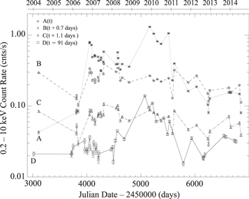
Figure 1. Total (0.2–10 keV) light curves of images A, B, C, and D of RX J1131–1231 shifted by the time delays estimated by Tewes et al. (2013). The total counts for images A and B have been corrected for pileup effects, while pileup is unimportant for images C and D. The new X-ray data begin after epoch 29 (2011 February, JD–2450000 = 5618).
Download figure:
Standard image High-resolution image
Figure 2. Total (0.2–10 keV) light curves of images A and B of QJ 0158–4325 shifted by the time delay of  = −14.5 days estimated by Faure et al. (2009). The new X-ray data begin after epoch 6 (2010 October, JD–2450000 = 5476).
Download figure:
Standard image High-resolution image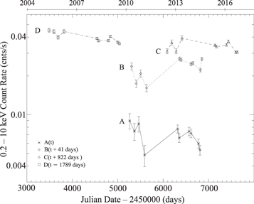
Figure 3. Total (0.2–10 keV) light curves of images A, B, C, and D of SDSS 1004+4112 shifted by the time delays estimated by Fohlmeister et al. (2008, 2016). We have added offsets of 0.01 counts s−1, 0.02 counts s−1, and 0.03 counts s−1 to the light curves of the images B, C, and D, respectively, for clarity. The new X-ray data begin after epoch 5 (2013 March, JD–2450000 = 6353).
Download figure:
Standard image High-resolution imageFor the spectral analyses, we followed the approach described in Chartas et al. (2012). We extracted events from circular regions with radii of 1.5 arcsec slightly off center from the images to reduce contamination from nearby images. The backgrounds were determined by extracting events within an annulus centered on the mean location of the images with inner and outer radii of 7.5 arcsec and 50 arcsec, respectively. Spectral fits were restricted to events with energies in the range 0.4–10 keV. Spectra with fewer than ∼200 counts were fit using the C statistic (Cash 1979),8 as appropriate for fitting spectra with low S/N. Spectra with a larger number of counts were fit using both the C and χ2 statistics.
Table 4. Properties of Samples
| Object | zs | zl | LBol/LEdd |

|

|

|
RE/ve | 10rg/ve | ve | μ |
|---|---|---|---|---|---|---|---|---|---|---|
| (M⊙) | (cm) | (cm) | (years) | (months) | (km s−1) | |||||
| RXJ1131 | 0.658 | 0.295 | 0.01–0.42 | 7.9–8.3 | 16.4 | 13.1–13.5 | 11.1 | 0.64–1.6 | 720 | 57 |
| QJ0158 | 1.29 | 0.317 | 0.4 | 8.2 | 16.5 | 13.4 | 18.0 | 1.5 | 600 | 5 |
| SDSS1004 | 1.73 | 0.68 | 0.05 | 8.6 | 16.4 | 13.8 | 9.4 | 2.9 | 785 | 70 |
Note. MBH and RE are the black hole mass and Einstein radius  with rg = GMBH/c2. RE/ve and rg/ve are the crossing times given the effective velocity ve (see Mosquera & Kochanek 2011). μ is the total flux magnification of the background quasar. For the estimate of the Eddington ratios, we assumed a 2–10 keV bolometric correction factor of κ2–10 keV ∼ 30.
Download table as: ASCIITypeset image
We fit the Chandra spectra for each epoch with a model that consists of a power law with neutral intrinsic absorption at the redshift of the source. Galactic column densities in the directions of RXJ1131, QJ0158, and SDSS1004 were fixed to NH = 3.60 × 1020 cm−2, NH = 1.88 × 1020 cm−2, and NH = 1.13 × 1020 cm−2, respectively (Dickey & Lockman 1990). Measurements of the differential X-ray absorption between images in lensed quasars SBS 0909+523, FBQS 0951+2635, and B 1152+199 by Dai & Kochanek (2009) have been used to successfully constrain the dust-to-gas ratio of the lens galaxies, and we plan to present the application of this method to our lens sample in a future paper. We next added one or two Gaussian emission lines to the model and tested for the significance of the added lines. The significance of the emission lines was determined by varying the energy and width of the iron line and its flux to calculate the χ2 of the fit as a function of the Fe line energy and iron line flux. In several cases, two emission lines are detected in a single spectrum. We record all cases where one or more emission lines are detected above the 90% and 99% confidence levels. Note that all these lines are detected in single epochs and not from stacked observations.
The confidence levels between the iron line flux and energy were created using the steppar command in XSPEC. As pointed out by Protassov et al. (2002), this approach may not apply for models near a boundary, such as in cases where the line flux normalization is constrained to have only positive values. To account for this limitation, we allowed the line flux normalization to obtain both positive and negative values. Protassov et al. (2002) proposed a more robust approach of estimating the significance of the shifted iron line based on Monte Carlo simulations to determine the distribution of the F statistic between different models. We followed this approach and constructed the simulated probability density distribution of the F statistic between spectral fits of models that included a simple absorbed power law (null model), and one that included one or two Gaussian emission lines (alternative model). Specifically, for each observed spectrum, we simulated 1000 data sets using the XSPEC fakeit command. We fit the null and alternative models to the 1000 simulated data sets and computed the F statistic for each fit. Finally from the Monte Carlo simulations we computed the probability of obtaining an F value larger than the one obtained from the fits of the null and alternative models to the observed spectrum. In Tables 5–7 we provide the F statistic between the null and alternative models and the probability of exceeding this value as determined from the Monte Carlo simulations.
Table 5. Properties of Shifted Fe Kα Line and Continuum in RX J1131–1231
| IDa | Imb | EFec | σFed | EWFee | NFef | Ncontg | Γ | cstath | dofi | Pj | Fk | PFl |
|---|---|---|---|---|---|---|---|---|---|---|---|---|
| (keV) | (keV) | (keV) | ||||||||||
| 4814 | 1 |

|

|

|

|

|

|
118.44 | 163 | 1 | 6.41 | <0.001 |
| 4814 | 2 |

|
<0.12 |

|

|

|

|
491.61 | 491 | 1 | 3.94 | 0.013 |
| 6912 | 2 |

|
<0.25 |

|

|

|

|
217.63 | 264 | 1 | 2.57 | 0.033 |
| 6913 | 1 |

|

|

|

|

|

|
116.63 | 152 | 1 | 4.35 | 0.003 |
| 6913 | 1 |

|
<0.12 |

|

|

|

|
116.63 | 152 | 1 | 4.34 | 0.004 |
| 6913 | 4 |

|
<0.15 |

|

|

|

|
52.03 | 77 | 0 | 7.81 | <0.001 |
| 6914 | 1 |

|

|

|

|

|

|
146.05 | 191 | 1 | 2.99 | 0.03 |
| 6914 | 2 |

|

|

|

|

|

|
175.40 | 234 | 0 | 11.96 | <0.001 |
| 6914 | 4 |

|
<0.60 |

|

|

|

|
92.55 | 95 | 1 | 2.24 | 0.1 |
| 6915 | 1 |

|

|

|

|

|

|
445.59 | 476 | 0 | 7.43 | <0.001 |
| 6915 | 1 |

|

|

|

|

|

|
445.59 | 476 | 1 | 7.42 | <0.001 |
| 6915 | 2 |

|
<0.07 |

|

|

|

|
333.73 | 343 | 0 | 6.65 | 0.001 |
| 6916 | 1 |

|
<0.30 |

|
15.8
|

|
1.58
|
440.07 | 479 | 1 | 4.30 | 0.001 |
| 6916 | 1 |

|
<0.50 |

|
16.2
|

|

|
440.07 | 479 | 1 | 4.36 | 0.002 |
| 7785 | 2 |

|
<0.10 |

|
12.8
|

|

|
295.14 | 312 | 0 | 9.40 | <0.001 |
| 7785 | 2 |

|
<0.10 |

|
7.0
|

|
1.86
|
295.14 | 312 | 1 | 9.40 | <0.001 |
| 7786 | 2 |

|
<0.20 |

|
9.7
|
89.0
|
1.70
|
331.99 | 384 | 1 | 4.64 | 0.003 |
| 7787 | 1 |

|

|

|
12.0
|

|

|
421.39 | 439 | 1 | 4.10 | 0.023 |
| 7787 | 1 |

|
<0.08 |

|
9.4
|

|

|
421.39 | 439 | 0 | 4.10 | 0.012 |
| 7788 | 1 |

|
<1.10 |

|
13.6
|
136.0
|

|
362.37 | 423 | 1 | 2.46 | 0.033 |
| 7789 | 1 |

|
<0.40 |

|
11.4
|
146.0
|

|
330.18 | 429 | 1 | 2.50 | 0.097 |
| 7789 | 2 |

|
<0.11 |

|

|

|

|
300.51 | 339 | 0 | 4.97 | 0.006 |
| 7790 | 3 |

|

|

|
13.0
|

|

|
25.96 | 29 | 1 | 4.46 | 0.007 |
| 7791 | 2 |

|
<0.10 |

|
5.82
|

|

|
294.67 | 340 | 1 | 2.08 | 0.04 |
| 7792 | 1 |

|
<0.50 |

|

|
145.0
|

|
342.32 | 407 | 1 | 2.46 | 0.073 |
| 7792 | 2 |

|

|

|

|

|

|
333.74 | 363 | 1 | 2.81 | 0.1 |
| 7793 | 1 |

|
<0.16 |

|
6.7
|

|
1.75
|
343.24 | 400 | 1 | 3.49 | 0.013 |
| 7793 | 2 |

|

|

|

|

|

|
312.71 | 346 | 1 | 2.44 | 0.023 |
| 7793 | 2 |

|
<0.55 |

|

|
84.4
|
1.83
|
312.71 | 346 | 1 | 3.47 | 0.0033 |
| 7793 | 3 |

|
<0.12 |

|
3.1
|
7.1
|

|
85.62 | 82 | 1 | 4.45 | 0.014 |
| 7794 | 2 |

|
<0.75 |

|
8.0
|

|

|
375.19 | 401 | 1 | 4.10 | 0.0033 |
| 7794 | 3 |

|
<0.14 |

|
3.0
|

|
1.89
|
166.94 | 221 | 1 | 3.76 | 0.01 |
| 9180 | 1 |

|

|

|
5.8
|

|

|
558.90 | 596 | 1 | 2.17 | 0.1 |
| 9180 | 3 |

|
<0.17 |

|

|
33.7
|

|
368.30 | 385 | 1 | 2.60 | 0.02 |
| 9181 | 1 |

|

|

|
18.2
|

|
1.65
|
632.52 | 638 | 0 | 6.16 | 0.001 |
| 9181 | 1 |

|
<0.12 |

|
7.2
|

|

|
632.52 | 638 | 1 | 6.14 | 0.001 |
| 9181 | 4 |

|
<0.12 |

|
1.5
|
12.0
|
1.84
|
192.77 | 227 | 1 | 2.2 | 0.02 |
| 9237 | 2 |

|
<0.13 |

|

|
90.2
|

|
560.80 | 584 | 1 | 2.07 | 0.037 |
| 9237 | 3 |

|

|

|

|
30.7
|

|
322.8 | 353 | 0 | 7.88 | <0.001 |
| 9237 | 4 |

|

|

|
3.3
|
6.8
|
1.7
|
183.75 | 195 | 0 | 5.56 | <0.001 |
| 9238 | 3 |

|

|

|
5.8
|

|

|
253.35 | 316 | 0 | 6.93 | 0.056 |
| 9238 | 3 |

|

|

|
2.8
|

|
1.85
|
253.35 | 316 | 0 | 2.88 | 0.033 |
| 9239 | 2 |

|

|

|
4.9
|

|

|
503.17 | 514 | 1 | 3.25 | 0.053 |
| 9240 | 2 |

|
<0.10 |

|

|

|

|
498.60 | 495 | 1 | 2.97 | 0.046 |
| 9240 | 2 |

|

|

|

|

|

|
498.60 | 495 | 1 | 4.18 | 0.026 |
| 9240 | 4 |

|
<0.06 |

|
1.8
|

|

|
228.56 | 260 | 1 | 3.75 | 0.063 |
| 11540 | 2 |

|
<0.10 |

|

|

|

|
678.26 | 681 | 1 | 3.52 | 0.03 |
| 11540 | 2 |

|
<0.12 |

|

|

|

|
678.26 | 681 | 1 | 3.01 | 0.057 |
| 11540 | 3 |

|

|

|

|

|

|
411.79 | 496 | 1 | 2.69 | 0.02 |
| 11542 | 1 |

|

|

|

|

|

|
963.88 | 822 | 0 | 8.30 | <0.001 |
| 11542 | 1 |

|

|

|

|

|

|
963.88 | 822 | 0 | 2.63 | 0.01 |
| 11542 | 2 |

|
<0.10 |

|

|

|

|
633.02 | 641 | 1 | 2.82 | 0.02 |
| 11543 | 1 |

|
<0.13 |

|

|

|

|
233.51 | 184 | 1 | 2.56 | 0.01 |
| 11543 | 1 |

|
<0.07 |

|

|

|

|
233.51 | 184 | 0 | 4.79 | 0.01 |
| 11543 | 3 |

|
<0.10 |

|

|

|

|
354.98 | 408 | 1 | 2.66 | 0.06 |
| 11543 | 3 |

|
<0.10 |

|

|

|

|
354.98 | 408 | 1 | 1.91 | 0.01 |
| 11544 | 3 |

|
<0.28 |

|

|

|

|
104.89 | 130 | 1 | 3.72 | 0.003 |
| 11545 | 3 |

|
<0.10 |

|

|

|

|
319.40 | 348 | 0 | 3.51 | 0.016 |
| 11545 | 3 |

|

|

|

|

|

|
319.40 | 348 | 0 | 6.09 | 0.004 |
| 12833 | 1 |

|
<0.2 |

|

|

|

|
492.66 | 577 | 0 | 4.80 | 0.005 |
| 12833 | 2 |

|

|

|

|

|

|
497.50 | 542 | 1 | 2.93 | 0.037 |
| 12833 | 3 |

|

|

|

|

|

|
337.96 | 346 | 1 | 2.98 | 0.036 |
| 12834 | 2 |

|

|

|

|

|

|
496.96 | 522 | 1 | 3.58 | 0.023 |
| 12834 | 4 |

|
<0.15 |

|

|

|

|
160.98 | 184 | 1 | 3.11 | 0.04 |
| 13962 | 1 |

|
<0.80 |

|

|

|

|
423.80 | 454 | 1 | 5.10 | 0.001 |
| 13962 | 1 |

|

|

|

|

|

|
423.80 | 454 | 0 | 5.10 | 0.002 |
| 13962 | 3 |

|

|

|

|

|

|
267.15 | 324 | 0 | 3.97 | 0.003 |
| 13962 | 4 |

|
<0.12 |

|

|

|

|
241.22 | 278 | 1 | 3.00 | 0.053 |
| 13963 | 1 |

|

|

|

|

|

|
401.43 | 403 | 1 | 4.32 | 0.007 |
| 13963 | 1 |

|
<0.30 |

|

|

|

|
401.43 | 403 | 1 | 4.32 | 0.01 |
| 13963 | 2 |

|

|

|

|

|

|
463.75 | 506 | 1 | 3.94 | 0.0033 |
| 13963 | 2 |

|

|

|

|

|

|
463.75 | 506 | 1 | 3.95 | 0.001 |
| 13963 | 3 |

|

|

|

|

|

|
240.66 | 294 | 1 | 3.01 | 0.013 |
| 14507 | 1 |

|
<0.14 |

|

|

|

|
268.03 | 282 | 1 | 3.28 | 0.03 |
| 14507 | 2 |

|

|

|

|

|

|
309.99 | 361 | 0 | 6.85 | <0.001 |
| 14507 | 3 |

|

|

|

|

|

|
150.66 | 198 | 1 | 3.93 | 0.002 |
| 14508 | 3 |

|

|

|

|

|

|
195.38 | 249 | 1 | 6.20 | 0.01 |
| 14510 | 4 |

|

|

|

|

|

|
46.62 | 61 | 1 | 6.81 | <0.001 |
Notes.
aChandra Observation ID. bImage numbers 1, 2, 3, and 4 correspond to images A, B, C, and D of RX J1131–1231. cObserved-frame energy of the shifted Fe line. dObserved-frame energy width of the shifted Fe line. eRest-frame equivalent width of the shifted Fe line. fFlux of the shifted Fe line in units of ×10−6 photons cm−2 s−1. gFlux density of the continuum in units of ×10−5 photons keV−1 cm−2 s−1 at 1 keV. hCash statistic. iDegrees of freedom. jP values of 0 and 1 correspond to confidence detection levels of the shifted Fe line of >99% and >90%, respectively. kF statistic between the null and alternative model. lThe probability of exceeding this F value as determined from the Monte Carlo simulations.Table 6. Properties of Shifted Fe Kα Line and Continuum in QJ 0158–4325
| IDa | Imb |
 c
c
|
σFed | EWFee | NFef | Ncontg | Γ | cstath | dofi | Pj | Fk | PFl |
|---|---|---|---|---|---|---|---|---|---|---|---|---|
| (keV) | (keV) | (keV) | ||||||||||
| 14487 | 2 |

|

|

|

|

|

|
101.83 | 111 | 1 | 3.56 | 0.040 |
| 14486 | 1 |

|

|

|

|

|

|
157.29 | 170 | 0 | 9.43 | <0.001 |
| 14485 | 1 |

|

|

|

|

|

|
166.84 | 191 | 0 | 6.50 | <0.001 |
| 14485 | 1 |

|

|

|

|

|

|
166.84 | 191 | 0 | 6.50 | <0.001 |
| 14484 | 1 |

|
<1.9 |

|

|

|

|
152.69 | 168 | 1 | 3.92 | 0.023 |
| 14484 | 2 |

|

|

|

|

|

|
68.33 | 80 | 1 | 4.92 | 0.006 |
| 11561 | 1 |

|

|

|

|

|

|
55.67 | 81 | 1 | 6.63 | 0.003 |
| 11561 | 2 |

|

|

|

|

|

|
30.53 | 41 | 1 | 2.91 | 0.037 |
| 11560 | 1 |

|

|

|

|

|

|
106.62 | 105 | 1 | 4.72 | 0.005 |
| 11557 | 1 |

|

|

|

|

|

|
76.04 | 88 | 1 | 5.07 | 0.008 |
Notes.
aChandra Observation ID. bImage numbers 1 and 2 correspond to images A and B of QJ 0158–4325. cObserved-frame energy of the shifted Fe line. dObserved-frame energy width of the shifted Fe line. eRest-frame equivalent width of the shifted Fe line. fFlux of the shifted Fe line in units of ×10−6 photons cm−2 s−1. gFlux density of the continuum in units of ×10−5 photons keV−1 cm−2 s−1 at 1 keV. hCash statistic. iDegrees of freedom. jP values of 0 and 1 correspond to confidence detection levels of the shifted Fe line of >99% and >90%, respectively. kF statistic between the null and alternative model. lThe probability of exceeding this F value as determined from the Monte Carlo simulations.Download table as: ASCIITypeset image
Table 7. Properties of Shifted Fe Kα Line and Continuum in SDSS 1004+4112
| IDa | Imb |
 c
c
|
σFed | EWFee | NFef | Ncontg | Γ | cstath | dofh | Pj | Fk | PFl |
|---|---|---|---|---|---|---|---|---|---|---|---|---|
| (keV) | (keV) | (keV) | ||||||||||
| 11549 | 4 |

|
<0.1 |

|

|

|

|
57.68 | 80 | 0 | 6.76 | 0.004 |
| 14495 | 2 |

|
<0.16 |

|

|

|

|
152.36 | 185 | 0 | 6.03 | 0.003 |
| 14495 | 4 |

|

|

|

|

|

|
124.95 | 150 | 0 | 14.3 | <0.001 |
| 14496 | 2 |

|
<0.12 |

|

|

|

|
185.30 | 200 | 1 | 4.12 | 0.02 |
| 14496 | 3 |

|
<0.20 |

|

|

|

|
159.62 | 196 | 0 | 9.07 | <0.001 |
| 14498 | 1 |

|
<0.37 |

|

|

|

|
94.73 | 124 | 0 | 7.59 | <0.001 |
| 14498 | 1 |

|
<0.11 |

|

|

|

|
94.73 | 124 | 0 | 7.54 | <0.001 |
| 14500 | 2 |

|
<0.10 |

|

|

|

|
178.21 | 204 | 1 | 4.59 | 0.008 |
Notes.
aChandra Observation ID. bImage numbers 1, 2, 3, and 4 correspond to images A, B, C, and D of SDSS 1004+4112. cObserved-frame energy of the shifted Fe line. dObserved-frame energy width of the shifted Fe line. eRest-frame equivalent width of the shifted Fe line. fFlux of the shifted Fe line in units of ×10−6 photons cm−2 s−1. gFlux density of the continuum in units of ×10−5 photons keV−1 cm−2 s−1 at 1 keV. hCash statistic. iDegrees of freedom. jP values of 0 and 1 correspond to confidence detection levels of the shifted Fe line of >99% and >90%, respectively. kF statistic between the null and alternative model. lThe probability of exceeding this F value as determined from the Monte Carlo simulations.Download table as: ASCIITypeset image
In Figure 4 we show a typical example of the Monte Carlo simulated distribution of the F statistic between fits of the null and alternative models to the observed spectrum of image C of RXJ1131 obtained in 2009 November 28 (obsid = 11540). We find that in this spectrum the probability of obtaining an F value larger than 2.69 is P = 0.018. In all cases listed in Tables 5–7, we confirm the significance of the shifted lines, and in all cases the significance inferred from the Monte Carlo analysis is similar or larger than the lower limits provided by the 90% and 99% χ2 confidence contours.
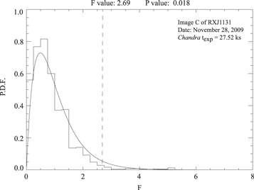
Figure 4. Monte Carlo simulated (histogram) and theoretical (smooth curve) probability density distributions of the F statistic between fits of models that included a simple absorbed power law (null model), and one that included one Gaussian emission line (alternative model) to the observed spectrum of image C of RXJ 1131 obtained in 2009 November 28 (obsid = 11540). We find that the probability of obtaining an F value larger than 2.69 is P = 0.018.
Download figure:
Standard image High-resolution imageIn Figures 5–7 we show typical examples of Fe Kα lines detected in the spectra of individual images and epochs from RXJ1131, QJ0158, and SDSS1004, respectively. We also show the respective χ2 contours of the detected lines. Tables 5–7 provide the line and continuum properties for all these detections. For RX J1131 we have 78 line detections out of the 152 spectra (38 epochs × 4 images) at >90% confidence, of which 21 lines are detected at >99% confidence. For the six Chandra observations of QJ0158 with exposure times of ∼19 ks, we detect 10 iron lines in 12 spectra (6 epochs × 2 images) at >90% confidence, of which three iron lines are detected at >99% confidence. For the 10 Chandra observations of SDSS1004, we detect the iron line in eight out of the 40 spectra (10 epochs × 4 images) at >90% confidence, of which six iron lines are detected at >99% confidence. For several closely separated observations, we detect energy shifts of the Fe Kα line in consecutive and closely separated epochs most likely produced by the same caustic crossing. For example, Figure 6 shows a likely caustic crossing in QJ0158 during 2013 December.

Figure 5. Left: spectra of images A, B, C, and D of RXJ1131 at four different epochs showing the shifted iron lines. The best-fit model is composed of a power law, one or two Gaussian lines, and Galactic and intrinsic absorption. Right: the 68%, 90%, and 99% χ2 confidence contours for the line energies and flux normalizations.
Download figure:
Standard image High-resolution image
Figure 6. Left: spectra of image A of QJ0158 at three different epochs showing the shifted iron lines. The best-fit models are composed of a power law, one or two Gaussian lines, and Galactic and intrinsic absorption. Right: the 68%, 90%, and 99% χ2 confidence contours for the line energies and flux normalizations.
Download figure:
Standard image High-resolution image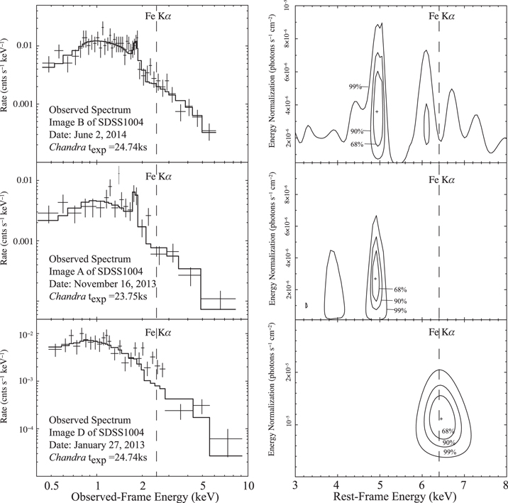
Figure 7. Left: spectra of images B, A, and D of SDSS1004 at three different epochs showing shifted iron lines. The best-fit models are composed of a power law, a Gaussian line, and Galactic and intrinsic absorption. The model for image D does not include the Gaussian line to better show the residual line emission near the instrumental edge at ∼2 keV. Right: the 68%, 90%, and 99% χ2 confidence contours for the line energies and flux normalizations.
Download figure:
Standard image High-resolution imageIn Figure 8 we show the generalized Doppler shift parameter g of the Fe line as a function of the equivalent width (EW) of the iron line in RXJ1131. We find a correlation between g and the EW with a Kendall's rank correlation coefficient of τ = 0.28 significant at >99.9% confidence. One possible explanation of this correlation is that blueshifted line emission is Doppler boosted, resulting in the observed EWs of the blueshifted lines being larger than the redshifted lines.
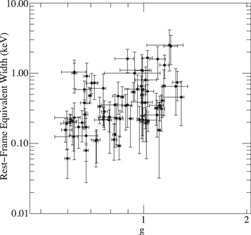
Figure 8. Fe line equivalent width as a function of the generalized Doppler shift parameter g for all images of RXJ1131. Only cases where the Fe line is detected at >90% confidence are shown.
Download figure:
Standard image High-resolution imageIn Figure 9 we show the flux of the Fe line as a function of the flux of the continuum, where the line flux is the normalization of the Gaussian line component of the best-fit model, and the continuum flux is the normalization of the power-law component of the best-fit model calculated at 1 keV. We find a strong correlation between the line and continuum fluxes, with a Kendall's rank correlation coefficient of τ = 0.5 that is significant at >99.9% confidence. The flux of the X-ray continuum relative to the Fe Kα line flux depends on a variety of accretion disk parameters and geometries, including the emissivity profile of the disk, the distance of the caustic from the black hole, the geometry of the corona, the geometry of the disk emission, the caustic crossing angle, and the inclination angle. Variations of the X-ray continuum and the Fe Kα line flux during caustic crossing have been simulated in Popović et al. (2006) for a variety of accretion disk parameters and geometries. These simulations indicate that once the magnification caustic has passed over the black hole, the microlensing magnifications of the line and continuum regions are similar, and both the line and continuum decay in a similar manner with distance from the black hole. This may explain part of the observed correlation between these quantities.

Figure 9. Flux of the Fe Kα line as a function of the continuum flux for Fe Kα lines detected at >90% confidence in RXJ1131. The line flux is the normalization of the Gaussian line component of the best-fit model. The continuum flux is the normalization of the power-law component of the best-fit model calculated at 1 keV.
Download figure:
Standard image High-resolution image3. The g and ΔE Distributions
We have recently developed a new technique based on microlensing that provides a robust constraint on the disk inclination angle and on the location of the ISCO, which in turn may provide an estimate of the spin of the black hole. Our technique is very simple. The stars near each lensed image produce magnification patterns with a characteristic Einstein radius of
where  is the mean mass of the lensing stars, the Dij are the angular diameter distances, and the subscripts L, S, and O refer to the lens, source, and observer, respectively.
These patterns contain caustic curves on which the magnification diverges. As the observer, lens, and source move, the quasar experiences a time-varying magnification whose amplitude is determined by the size of the source, with larger sources showing lower amplitudes because they more heavily smooth the magnification patterns (e.g., Wyithe et al. 2000, 2002; Kochanek 2004). If the X-ray emission is dominated by the inner edge of the disk, then the characteristic source size is rs ∼  ∼ 1015(MBH/109 M⊙) cm where rg = GMBH/c2. The effective source velocity across the pattern for our three quasars is in the range ve ∼ 600–785 km s−1 (see Mosquera & Kochanek 2011), leading to two characteristic timescales for variability: the Einstein crossing time RE/ve, typically several years, and the source crossing time rs/ve, typically a few months (see Table 4).
As a caustic crosses the accretion disk, it differentially magnifies the Fe Kα line emission to produce changes in the line profile. We will observe these as shifts in the line energy that we use to calculate the distribution of the fractional energy shifts g = Eobs/Erest (the "g distribution"). We first present an analytic estimate of the energy shift of the iron line caused by microlensing and compare these analytic estimates with the observed energy shifts. Numerical simulations of microlensing events are presented later in the section. The observed energy, Eobs, of a photon emitted near the event horizon of a supermassive black hole will be shifted with respect to the emitted rest-frame energy, Eemit, due to general relativistic and Doppler effects. The ratio between the observed energy and the emitted rest-frame energy is often referred to as the generalized Doppler shift and is defined as
where the Doppler factor δ is
 ,
,  ,
,  , and θc is the angle between the direction of the orbital velocity vϕ of the emitting plasma and our line of sight, neglecting the general relativistic effect of the bending of the photon trajectories and relativistic aberration (see appendix for details). In Section 4 we compare our analytic estimate of the generalized Doppler factor g with the observed limits of the g distributions of RXJ1131.
We next use numerical simulations to evaluate if the microlensing of the X-ray emission from a mass-accreting supermassive black hole can indeed produce energy spectra similar to the observed ones. The simulations assume that RXJ1131 accretes through a standard geometrically thin, optically thick accretion disk (Novikov & Thorne 1973; Shakura & Sunyaev 1973) described by the analytical general relativistic equations of Page & Thorne (1974). This assumption seems to be well justified for two reasons. Sluse et al. (2012) estimate that the black hole of RXJ1131 has a mass MBH between 8 × 10⁷ M⊙ and 2 × 10⁸ M⊙ and a bolometric luminosity of LBol ≈ 1045 erg s−1. The inferred ratio of LBol/LEdd is therefore expected to range between 0.01 and 0.42. It is therefore likely that RXJ1131 is accreting in the regime in which accretion is believed to be dominated by a geometrically thin, optically thick accretion disk (see, e.g., the discussion in McKinney et al. 2014). General relativistic (radiation) magnetohydrodynamic simulations indicate that the analytical equations describe accretion disks reasonably accurately (Kulkarni et al. 2011; Noble et al. 2011; Penna et al. 2012; Sa̧dowski 2016). However, optical and UV observations of microlensing events in quasars indicate that accretion disks are larger than predicted by thin-disk theory (Morgan et al. 2010), and similar discrepancies are found using measurements of continuum lags in the nearby Seyferts NGC2617 (Shappee et al. 2014) and NGC5548 (Edelson et al. 2015; Fausnaugh et al. 2016).
We use a general relativistic ray-tracing code (Krawczynski 2012; Beheshtipour et al. 2016; Hoormann et al. 2016) to track photons of initially unspecified energy from a lamppost corona (Matt et al. 1991) to the observer, accounting for the possibility that the photons impinge on the accretion disk and either reflect or prompt the emission of Fe Kα photons. The compactness of the corona has been observationally and independently confirmed via microlensing (e.g., Pooley et al. 2007; Morgan et al. 2008, 2012; Chartas et al. 2009, 2016; Dai et al. 2010; Mosquera et al. 2013; Blackburne et al. 2014, 2015; MacLeod et al. 2015) and reverberation studies (Fabian et al. 2009; de Marco et al. 2011; Kara et al. 2013, 2014, 2016; Cackett et al. 2014; Emmanoulopoulos et al. 2014; Uttley et al. 2014). The reverberation studies in many cases constrain the distance between the corona and central black hole to lie in the range of 3–10rg.
In our simulations, the corona is located above the black hole at a radial Boyer–Lindquist (BL) coordinate r = 5 rg slightly offset from the polar axis (θ = 10°) and emits isotropically in its rest frame. The zero component of the wave vector kμ of the photon packet is proportional to the energies of the photons, and we assume that the corona emits a power-law SED with a photon number power law of dN/dE ∝ E−Γ with Γ = 1.75. After transforming the photon packet's wave vector into the global BL coordinates, the code integrates the geodesic equation until the photon packet either comes too close to the black hole horizon (when we assume it will enter the black hole), impinges on the accretion disk, or arrives at a fiducial stationary observer at robs = 10,000 rg.
We assume that the accretion disk extends from the ISCO to 100 rg. We use simple prescriptions for treating the absorption, reflection, and reprocessing in the disk's photosphere. If a photon packet hits the disk, it is absorbed with probability pabs, it scatters with probability  , or it prompts the emission of a monoenergetic Fe Kα photon with probability
  so that
  . Although we use pabs = 0.9 and R = 1, the results do not depend strongly on the specific choice (see Ross & Fabian 2005; García et al. 2013, for more detailed treatments). The Fe Kα photons are always emitted with an energy of 6.4 keV in the rest frame of the accretion disk with a statistical weight that depends on the net redshift or blueshift g incurred between the emission of the photon in the corona and its absorption in the accretion disk. More specifically, the weight is given by
  with
with

Here,  and
and  denote the four velocities of the corona and the accretion disk plasmas, respectively, and
  and
and  denote the photon packet wave vectors in the rest frames of the corona plasma and accretion disk plasma (before the absorption of the photon packet), respectively. The scattering model is based on the classical treatment by Chandrasekhar (1960) of scattering by an indefinitely deep electron atmosphere. Tracking photon packets forward in time allows us to model multiple interactions of the photon packets with the accretion disk before or after a photon packet prompts the emission of a Fe Kα photon packet (see also Schnittman & Krolik 2009, 2010, and references therein). Our treatment neglects the possibility that Fe Kα photons return to the accretion disk and may prompt the emission of another Fe Kα photon, but this is a very small correction. When a photon packet reaches the observer, its wave vector is transformed from the global BL frame into the reference frame of a coordinate stationary observer. Although we simulated 10 million photon packets for a range of black hole spins (a = 0, 0.1, 0.2, ..., 0.9, 0.95, 0.98, 0.998), we will show here only example results for a = 0.3. The results for other black hole spins will be presented in a forthcoming paper (H. Krawczynski et al. 2017, in preparation).
In this paper we use the general parameterization of the microlensing magnification μ close to caustic folds above the magnification μ0 outside the caustic (see, e.g., Schneider et al. 1992; Chen et al. 2013):
with y⊥ giving the position of the origin of the emission in the source plane along a coordinate axis perpendicular to the fold, K is the caustic amplification factor, and H is the Heaviside function (i.e., H(y⊥) = 0 for y⊥ < 0 and H(y⊥) = 1 for y⊥ ≥ 0). For microlensing by a random field of stars, K/μ0 is given by (Witt et al. 1993; Chartas et al. 2002)

where β is a constant of order unity, and ζE is the Einstein radius for stars of average mass  In this paper, we show results for β = 0.5 and ζE = 1640 rg, corresponding to
  and MBH = 108 M⊙. For each simulated black hole spin, we simulate caustic crossings at crossing angles θc (the angle between the normal of the caustic fold and the black hole spin axis) between 0° and 360° in 20° steps and for −30 rg to +30 rg offsets of the caustic from the center of the black hole. An angle of θc = 0 corresponds to a caustic fold perpendicular to the black hole spin axis with the positive side of the caustic (the side with μ > 1) pointing in the θ = 0 direction.
The left panel of Figure 10 shows a 2D map of the surface brightness of the Fe Kα line emission in the source plane after convolving it with a caustic magnification (a = 0.3, i = 825, θc = π/2). An actual observer would see a different surface brightness distribution, as Figure 10 accounts for the flux magnification but not for the image distortion caused by the gravitational lensing. The magnification pattern of Equation (5) can clearly be recognized by a sudden jump from μ = 1 to μ ≫ 1, followed by the gradual return of the magnification to μ ≈ 1. The right panel shows the resulting Fe Kα energy spectrum. Similar to the Chandra energy spectra shown in Figure 5, the simulated energy spectrum exhibits two distinct peaks. Scrutinizing similar maps and energy spectra for different caustic crossing angles and offsets reveals that double peaks appear naturally (but not only) when the positive side of the caustic magnifies lower surface brightness emission that is not as strongly Doppler boosted as the emission from the portions of the accretion disk approaching the observer with near-relativistic speed.

Figure 10. The left panel shows an image of the surface brightness of the Fe Kα line emission as seen by an observer at 104 rg and an inclination of i = 825 from a black hole of spin a = 0.3 for a caustic crossing angle of θc = π/2. The surface brightness scale is logarithmic with an arbitrary absolute scale. The surface brightness exhibits a left–right asymmetry owing to the motion of the accretion disk plasma toward (left) or away from (right) the observer. The right panel shows the resulting energy spectrum of the Fe Kα emission in the rest frame of the source.
Download figure:
Standard image High-resolution imageFigure 11 shows a 2D map of the g factors of the Fe Kα photons for the same parameters as in Figure 10. The image clearly shows the highest blueshifts from regions of the accretion disk moving toward us with near-relativistic speed.
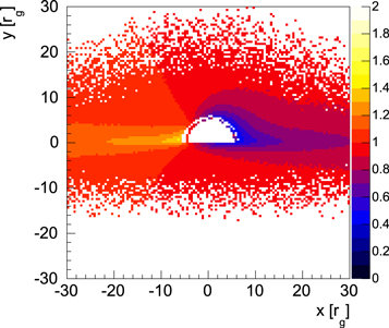
Figure 11. Map of the g factors of the Fe Kα emission originating in the accretion disk. The net g factors result from the motion of the accretion disk plasma relative to the observer shown in Figure 9 and the propagation of the photon through the curved spacetime for the same parameters as were used in Figure 9.
Download figure:
Standard image High-resolution imageNote that the gravitational redshift wins over the Doppler blueshift very close to the event horizon. The minimum and maximum g values are 0.42 and 1.4, respectively, and are in good agreement with the observed values. We have explored the dependence of the observed g values on the coronal height. We find that for larger coronal heights the g distribution becomes narrower, as the inner edge of the disk is not illuminated as much as it is for low coronal heights, and thus the extreme g-factor emission is less intense. We conclude that for larger coronal heights the observed gmax value for RXJ1131 would imply even higher inclinations.
We analyzed the energy spectra for all caustic crossing angles and offsets with an algorithm identifying the most prominent peaks and fitting them with Gaussians. The algorithm first finds the highest peak in the photon number energy spectrum (dN/dE) and then searches for an additional peak that rises more than 10% above the valley between the two peaks. Figure 12 shows the distribution of all the peak energies found in this way (singles and doubles). Figure 13 presents all simulated and observed double peak energies. Although a statistical analysis of the results is outside the scope of this paper, we will see in Section 4 that the simulated results do resemble the observed ones at least on a qualitative level.

Figure 12. Simulated distribution of the single and double peak Fe line energies for a black hole with a spin of a = 0.3 seen at an inclination of i = 825.
Download figure:
Standard image High-resolution image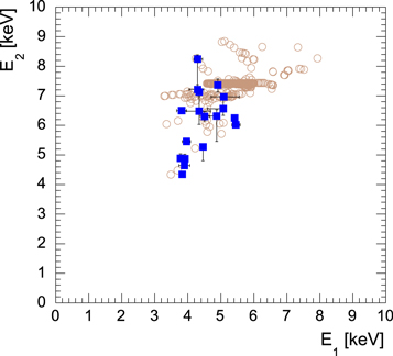
Figure 13. Scatter between the peak energies of simulated (open circles) and observed (solid squares) double-peaked line profiles. The simulations are for a black hole with a spin of a = 0.3 seen at an inclination of i = 825.
Download figure:
Standard image High-resolution image4. Results
We detect shifted and broadened Fe Kα lines in almost every image of RXJ1131 that has an exposure time of >20 ks, as shown in Figure 5 and Table 5. Relativistically broadened Fe Kα lines detected in the spectra of unlensed AGNs are produced from emission originating from the entire inner accretion disk. In contrast, the microlensed Fe Kα lines in the spectra of lensed AGNs are produced from a relatively smaller region on the disk that is magnified as a microlensing caustic crosses the disk. We therefore expect microlensed Fe Kα lines to be in general narrower and with larger EWs than those detected in unlensed AGNs. The observed EWs of Fe Kα lines in RXJ1131 are significantly affected by microlensing of both the direct continuum emission of the corona and the reflected line and continuum from the disk. The relative microlensing magnification of the direct and reflected emission was simulated in Popovic et al. (2006) for a variety of accretion disk parameters and geometries. Chen et al. (2012) compared the properties of a sample of lensed quasars with nonlensed ones and found that the EWs of the Fe lines detected in lensed quasars are systematically higher than those found in nonlensed ones, and this can be explained as the result of microlensing of both the continuum and line emission.
The presence of these energy shifts is evidence that most of the shifted iron line emission detected in RXJ1131 does not originate from reflection from a torus or other distant material but from material near the event horizon of the black hole. The evolution of the energy and shape of the Fe Kα line during a caustic crossing depends on the ISCO, spin, inclination angle of the disk, and caustic angle. The extreme shifts are produced when the microlensing caustic is near the ISCO of the black hole. Measurements of the distribution of the fractional energy shifts g = Eobs/Erest of the Fe Kα line due to microlensing therefore provide a powerful limit on the g distribution that can be used to estimate the ISCO, spin, and inclination angle of the disk.
In Figure 14 we show the g distribution (multiplied by the rest-frame energy of the Fe Kα line, Erest = 6.4 keV) of the Fe Kα lines with >90% and >99% detections in RXJ1131 for all images and epochs. One important feature of this iron line energy-shift distribution is the significant limits of the distribution at rest-frame energies of Emin = 3.78 keV and Emax = 8.24
 keV, where the error bars for both Emin and Emax are at the 90% confidence level, for iron lines detected at >90% confidence. These limits represent the most extremely redshifted and blueshifted Fe Kα lines. If we interpret the largest energy shifts as being due to X-ray emission originating close to the ISCO, we obtain upper limits on the size of the ISCO and inclination angle of RXJ1131. In Figure 15 we show the g distribution for the individual images of RXJ1131. The apparent differences of the distributions between images can be a result of several factors, including the differences in the frequency of microlensing along different lines of sight, the differences in the S/N of the spectra (D being the faintest image), and differences in caustic crossing angles. The observed g distributions of Figures 14 and 15 closely resemble the simulated distribution of all peaks shown in Figure 12.
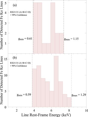
Figure 14. Distribution of the Fe Kα line energies for all images and all 38 epochs of data for RXJ1131. Only cases where the iron line is detected at >99% (a) and at >90% confidence (b) are shown. The vertical lines mark the extreme limits of the distribution used to determine upper limits on the ISCO and inclination angle.
Download figure:
Standard image High-resolution image
Figure 15. Distribution of the Fe Kα line energies for the individual images A, B, C, and D and all 38 epochs of data for RXJ1131. Only cases where the iron line is detected at >90% confidence are shown.
Download figure:
Standard image High-resolution imageThe energies of photons emitted from a ring at the ISCO are bounded by maximum and minimum values, gmax and gmin, of the generalized Doppler shift. The maximum blueshift of the Fe line places a constraint on the inclination angle. Specifically, for RXJ1131 the measured generalized Doppler factor gmax = 1.29 ± 0.04 (90% confidence) constrains the inclination angle to be ≳64°, for any values of the spin parameter and caustic crossing angle, as shown in Figure 16, assuming that the thin accretion disk extends all the way down to the ISCO. If we also require that the measured gmin and gmax shifts are produced by photons emitted from the same radius, then the inclination angle is required to be i ≳ 76° for photons emitted from a radius of r ∼ 8.5 rg for any values of the spin parameter and caustic crossing angle, as also shown in Figure 16. We conclude that the current observed values of gmin and gmax place an upper limit on the ISCO radius of rISCO ≲  and a disk inclination angle of i ≳ 76°. If we only consider energy shifts detected above the 99% confidence level, the upper limit on the ISCO radius is rISCO ≲
  and the lower limit on the disk inclination angle is i ≳ 55°.

Figure 16. Extremal shifts of the Fe Kα line energy for spin values ranging between 0.098 and 0.998 in increments of 0.1. Horizontal lines represent the observed values of g = Eobs/Erest of the most redshifted and blueshifted Fe Kα lines from all 38 epochs and all images of RXJ1131. The extreme g values are for Fe Kα lines detected at >90% confidence. (a) The extremal shifts for an inclination angle of i = 64°. (b) The extremal shifts for an inclination angle of i = 76°. The inner radius of the accretion disk is constrained to be rISCO < 
Download figure:
Standard image High-resolution imageThe gmin value provides an estimate of the radius of the emission region closest to the center of the black hole. If one assumes that the innermost emission region is near the ISCO radius, one can obtain a constraint on the spin of the black hole based on the relation between ISCO and spin. However, recent 3D MHD simulations of thin accretion disks indicate slight bleeding of the iron line emission to the region inside the ISCO (e.g., Reynolds & Begelman 1997). Reynolds & Fabian (2008) have attempted to estimate the systematic error on inferred black hole spin using the relativistic iron line method to infer the true spin of a black hole. They find that the systematic errors can be significant for slowly spinning black holes but become appreciably smaller as one considers more rapidly rotating black holes. In a future paper we plan to perform an analysis of the systematic errors on inferred black hole spin derived from the g distribution method and from the distribution of energy separations of double peaked lines caused by the possible bleeding of the iron line emission to the region inside the ISCO.
We also detect energy shifts in the Fe line in QJ0158 and SDSS1004, but they have not been monitored as frequently as RXJ1131. In Figure 17 we show the g distributions of the Fe Kα lines with >90% confidence detections in QJ0158 and SDSS1004 for all images and epochs. These g distributions of QJ0158 and SDSS1004 are too sparsely populated to provide statistically significant constraints on the ISCO radii with the available data but demonstrate that these lenses also have microlensed Fe emission.
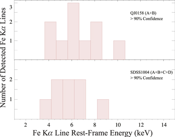
Figure 17. Distribution of the Fe Kα line energies for all images of QJ0158 (top, 12 epochs) and SDSS1004 (bottom, 10 epochs). Only cases where the iron line is detected at >90% confidence are shown.
Download figure:
Standard image High-resolution imageIn several observations we detect two shifted Fe lines, as shown in Figures 6 and 7. Specifically, the numbers of detected double lines in the spectra of images A, B, C, and D of RXJ1131 are 9, 5, 3, and 0, respectively. All of the cases are detected at the >90% confidence level. In the following, we call energy spectra with one peak "singles" and energy spectra with two peaks "doubles." We searched for possible correlations between the energies of the doubles. A moderately significant correlation, with a Kendall's rank correlation coefficient of τ = 0.6 and a significance of >98% confidence, is detected between the observed Emin and Emax values in image A. The observed energies of the double lines detected in the spectra of image A and the spectra of all images are shown in Figures 18 and 19, respectively. We performed a straight-line least-squares fit to the data with the FITEXY routine (Press et al. 1992), which takes into account errors in both coordinates. Based on the magnification maps of RX J1131–1231 (see Figures 4–6 of Dai et al. 2010), we expect a limited range of caustic crossing angles over ∼10 years. Any change in the caustic crossing angle over time will contribute to the scatter in the observed Emin and Emax values of doubles. The scatter in the Emin and Emax values detected in all images is even larger, as we would expect from the differences in the caustic structures and their directions of motion in different images (Kendall's τ = 0.4, significant at >97% confidence).
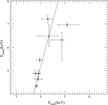
Figure 18. Rest-frame energies of the shifted double Fe lines detected in image A of RXJ1131 at the >90% confidence level. We also show the straight-line least-squares fit to the data in the solid line.
Download figure:
Standard image High-resolution image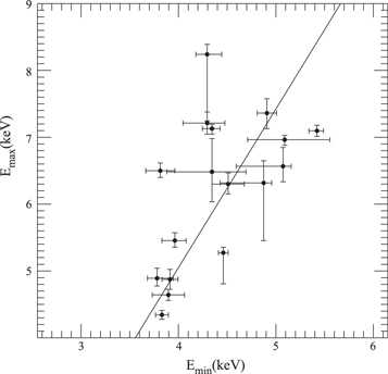
Figure 19. Rest-frame energies of the shifted double Fe lines detected in all images of RXJ1131 at the >90% confidence level. We also show the straight-line least-squares fit to the data in the solid line.
Download figure:
Standard image High-resolution imageIn Figure 20 we show the ΔE distribution of the rest-frame energy separations for the Fe line pairs detected in all images of RXJ1131 at the >90% confidence level, where ΔE =  and Emax and Emin are the rest-frame energies of the shifted lines. As we discussed in Section 3, our numerical simulations show that the peak energy of the ΔE distribution depends strongly on the spin parameter. Specifically, our simulations indicate that the ΔE distributions of RX J1131–1231 for input spin parameters of a = 0 and a = 0.98 peak at 1.8 ± 0.2 keV and 3.2 ± 0.2 keV, respectively. We find that the maximum of the observed ΔE distribution of RX J1131–1231 peaks at ∼3.5 ± 0.2 keV, implying a spin parameter of a ≳ 0.8. Additional observations of RXJ1131 will provide more representative and complete g and ΔE distributions and place tighter constraints on the disk inclination angle, the ISCO radius, and the spin.

Figure 20. Observed distribution of the rest-frame energy separations for shifted double Fe lines detected in all images of RXJ1131 at the >90% confidence level.
Download figure:
Standard image High-resolution image
5. Discussion and Conclusions
Our systematic spectral analysis of all the available Chandra observations of lensed quasars RXJ1131, QJ0158, and SDSS1004 has revealed the presence of a significant fraction of lines blueshifted and redshifted with respect to the energy of the expected Fe Kα fluorescence line. We interpret these energy shifts as being the result of ongoing microlensing in all of the images. This seems logical given the prior detections of microlensing of the optical, UV (e.g., Blackburne et al. 2006; Fohlmeister et al. 2007; Morgan et al. 2008; Motta et al. 2012; Fian et al. 2016), and X-ray continuum (e.g., Chartas et al. 2009, 2012, 2016; Dai et al. 2010; Chen et al. 2011, 2012) in all three sources. We consider several alternative scenarios and examine whether they can explain the observed shifted iron lines.
(a) Nonmicrolensed emission from hot spots and patches from an inhomogeneous disk. Redshifted Fe emission lines have been reported in observations of a few bright Seyfert galaxies (i.e., Iwasawa et al. 2004; Turner et al. 2004, 2006; Miller et al. 2006; Tombesi et al. 2007). Correlated modulation of redshifted Fe line emission and the continuum were reported in NGC 3783 (Tombesi et al. 2007). Specifically, the spectrum of NGC 3783 shows, in addition to a core Fe Kα line at 6.4 keV, a weaker redshifted wing and redshifted Fe emission line component. The redshifted line and wing appear to show an intensity modulation on a 27 ks timescale similar to that of the 0.3–10 keV continuum. Tombesi et al. (2007) argue that the lack of Fe line energy modulation disfavors the orbiting flare/spot interpretation for NGC 3783. We note that the relative intensity of the core Fe line to the redshifted Fe line component in NGC 3783 is about a factor of 9. The core Fe Kα line has an EW of about 120 eV and the redshifted line of ∼13 eV. Redshifted lines are also reported to be present in the spectrum of Mrk 766 (Turner et al. 2004, 2006), where a weak component of the Fe line with an EW of  eV shows a periodic variation of photon energy. The proposed scenario by Turner et al. (2006) is that the energy variation is caused by a hot spot on the disk within ∼100 rg orbiting with a period of about ∼165 ks. The average spectrum of Mrk 766 shows a broad iron line center near 6.7 keV with an EW of about 90 eV (possibly from reflection off an ionized disk) and a narrower component at 6.4 keV (possibly from reflection from distant material).
The shifted Fe lines detected in our gravitationally lensed quasar sample have very different properties from those reported in NGC 3783 and Mrk 766, while our our microlensing interpretation is consistent with the observed properties of the energy-shifted lines. Specifically, the EWs of the energy-shifted lines in the lensed quasar sample range from EW = 500 to 3000 eV compared to the EW = 13 eV and EW = 15 eV in the shifted lines detected in NGC 3783 and Mrk 766, respectively. Nonmicrolensed emission from hot spots and patches from an inhomogeneous disk lie below the detection threshold of the individual spectra of the lensed quasars. The nonmicrolensed emission from the Fe Kα line at 6.4 keV is not detected in individual spectra of RX J1131–1231, but is detected in the stacked spectra of RX J1131–1231 with  keV and EW =
  eV (Chartas et al. 2012, 2016). In the cases of Seyfert galaxies NGC 3783 and Mrk 766, the redshifted weak Fe lines are always accompanied by a significantly stronger core component near 6.4 keV, whereas this is not the case for the lensed quasars. Another point supporting the microlensing interpretation is the detection of a significant number of double lines in RX J1131–1231, as predicted in our numerical simulations of magnification caustics crossing an accretion disk. The intensities of these doubles are not consistent with nonmicrolensed Fe emission from hot spots and patches from an inhomogeneous disk.
(b) Possible intrinsic absorption mimicking two apparent lines in RX J1131–1231. Our analysis of the 4 × 38 spectra of RX J1131–1231 does not find any significant intrinsic absorption of the continuum spectra (Chartas et al. 2012), and there are no absorption lines detected in the spectra that contain doubles.
(c) Possible ionization of accretion disk. In Figure 9 of Chartas et al. (2012) we showed a stacked spectrum of image C of RXJ1131 covering a period of about seven years filtering for epochs where microlensing was not significant in this image. A significant Fe Kα line is detected in the stacked spectrum of image C at an energy of  keV with an EW of
  eV. This detected energy of the Fe Kα line in image C is consistent with the presence of a nonionized disk in RXJ1131. The expected energy of the iron line for an ionized disk would be 6.67 keV (He-like Fe) or 6.97 keV (H-like iron).
We conclude that the variability in the flux and energy of the iron line detected in the Chandra observations of RXJ1131, QJ0158, and SDSS1004 is due to ongoing microlensing of all of the images.
Large magnification events are typically inferred from the departure of the time-delay-corrected flux ratios of images from a constant, and images that show significant uncorrelated variability are significantly affected by microlensing. We note, however, that a relatively large number of the shifted Fe lines were found in images that do not show significant variability of their flux ratios or significant uncorrelated variability. This implies that the line profiles found using stacked spectra taken over multiple epochs, even when excluding spectra from images that show variability of their flux ratios, are also distorted by microlensing, and that applying the relativistic Fe Kα method as used to analyze local Seyferts will not lead to reliable results. Any apparent broadening of the iron line in a stacked spectrum of a lensed quasar is a combination of both microlensing and the relativistic blurring seen in unlensed Seyferts. The average stacked spectrum of a microlensed quasar differs significantly, especially near the Fe Kα line, from that of an unlensed one. The main reason for this difference is that the reflection and direct (coronal) components of a stacked spectrum of a microlensed quasar are not a simple, uniform magnification of the reflection and direct components of unlensed quasars. Caustic magnification patterns (e.g., see Figures 12–16 of Kochanek 2004) move along a certain direction with respect to the source (that differs between images), and the caustic magnification is not uniform. Stacked spectra of lensed quasars will thus not result in uniformly magnified reflection and direct spectral components but will produce spectra that have been selectively magnified by caustics moving along a limited range of caustic crossing angles. The caustic magnification factor K will also vary between caustic crossings, making the stacked spectrum deviate even more than a uniformly magnified quasar spectrum.
We summarize our main conclusions from the X-ray observations of RXJ1131, QJ0158, and SDSS1004 as follows:
(1) Redshifted and blueshifted Fe lines with rest-frame EWs ranging between 500 and 3000 eV are detected in the individual epoch spectra of lensed quasars RXJ1131, QJ0158, and SDSS1004. We interpret these energy shifts as the result of microlensing of Fe line emission within ∼20 rg of the black hole.
(2) The g distribution of the observed energy shifts in RXJ1131 is compared to analytic and numerical models, and both models provide similar constraints on accretion disk parameter. Specifically, the maximum value of gmax =  constrains the inclination angle to be i ≳ 76°, and the minimum value gmin = 0.59 constrains
  . If we only consider energy shifts detected above the 99% confidence level, the upper limit on the ISCO radius is
  and the lower limit on the disk inclination angle is i ≳ 55°. One of the strengths of the g-distribution method is that the energies of the shifted Fe lines are more robustly detected than the extreme weak red wings of the relativistic Fe Kα line that are found mostly in nearby Seyfert galaxies. For example, the energies of the shifted lines are not sensitive to the modeling of the underlying continuum, while the shape of the relativistic Fe Kα red wing is very sensitive to the continuum model. The g-distribution method can be applied to infer the inclination angles, ISCO radii, and spins of distant quasars, where the relativistic Fe Kα red wing is typically too faint to constrain these parameters in distant quasars. One of the weaknesses of the g-distribution method is that there are additional model parameters related to describing the gravitational lens.
(3) Several spectra show two shifted Fe lines, which we refer to as doubles. The peak energies of the doubles are moderately correlated. Our numerical simulations reproduce the double lines during caustic crossings, and we find that the distribution of the separations of the peak energies is strongly dependent on the spin parameter. The maximum of the observed ΔE distribution of RX J1131–1231 peaks at ∼3.5 ± 0.2 keV, suggesting a high spin parameter. Although a statistical analysis of the results still needs to be performed, inspection of the mean energy, peak energy, and shape of the distribution indicates a rather high value of the spin a ≳ 0.8. The available ΔE distribution of RX J1131–1231 is sparsely populated, and additional observations are required to better constrain the peak energy of this distribution and infer the spin parameter more accurately.
(4) We find several correlations in the microlensed spectra of RXJ1131, and the results are summarized in Table 8. Specifically, we find a correlation between the rest-frame EW of the iron lines and the generalized Doppler shift parameter g of the iron line (τ = 0.28, P > 99.9%). The flux of the shifted Fe line is found to be correlated with the flux of the continuum for Fe Kα lines detected at >90% confidence in all images of RXJ1131 (τ = 0.5, P > 99.9%). The energies of the doubles in image A are also found to be correlated (τ = 0.6, P > 98%).
Table 8. Correlation Results of RX J1131–1231
| TEST | QUANTITY I | QUANTITY II |
 a
a
|
STATISTIC | CHANCE PROBABILITY |
|---|---|---|---|---|---|
| Spearman's (ρ) | Eminb | Emaxb | 9 | 0.78 | 0.015 |
| Kendalls's (τ) | Eminb | Emaxb | 9 | 0.61 | 0.022 |
| Spearman's (ρ) | Eminc | Emaxc | 17 | 0.52 | 0.032 |
| Kendalls's (τ) | Eminc | Emaxc | 17 | 0.39 | 0.031 |
| Spearman's (ρ) | EWFe | g | 78 | 0.42 | 1.6 × 10⁻⁴ |
| Kendalls's (τ) | EWFe | g | 78 | 0.28 | 2.4 × 10⁻⁴ |
| Spearman's (ρ) | NFe | Ncont | 78 | 0.69 | 4.4 × 10⁻¹² |
| Kendalls's (τ) | NFe | Ncont | 78 | 0.50 | <1 × 10⁻¹² |
Notes. Spearman's (ρ) and Kendalls's (τ) rank correlations of two sample populations labeled QUANTITY I and QUANTITY II.
aThe number of elements in the sample. bRest-frame energies of the shifted double Fe lines in image A detected at the >90% confidence level. cRest-frame energies of the shifted double Fe lines in all images detected at the >90% confidence level.Download table as: ASCIITypeset image
(5) Our numerical simulations of microlensing caustic crossings reproduce the observed distribution of energy of single and double shifts in microlensed spectra and predict the correlations observed in the spectra.
Scheduled future monitoring observations with Chandra of the lensed quasars RXJ1131, QJ0158, SDSS1004, and Q 2237+0305 with sufficiently long exposure times to improve the significance of the detections will provide more representative and complete distributions of the generalized Doppler shift g values of the Fe Kα line in these objects. The g-distribution method and modeling of doubles are expected to provide robust constraints on inclination angle, the ISCO radii, and spins of the black holes of these distant lensed quasars. With the Large Synoptic Survey Telescope coming online in the near future, we expect ∼4000 new lensed systems to be discovered, opening up the possibility of measuring black hole and accretion disk parameters over a wide range of redshifts and quasar Eddington ratios LBol/LEdd.
We acknowledge financial support from NASA via the Smithsonian Institution grants SAO GO4-15112X, GO3-14110A/B/C, GO2-13132C, GO1-12139C, and GO0-11121C. C.W.M. gratefully acknowledges support from NSF Award AST-1211146. C.S.K. is supported by NSF grant AST-1515876.
Appendix: Calculating the Generalized Doppler Shifts g
The generalized Doppler shifts g were calculated for the case of a spinning black hole (Kerr 1963) using the formalism described in Bardeen et al. (1972), Müller & Camenzind (2004), and Karas & Sochora (2010). The azimuthal velocity is

where  and
and  are given by


For r > rms, a Keplerian velocity profile is assumed, and
For r ≤ rms, a constant specific angular momentum is assumed, and the angular velocity Ω is given by

where
All quantities with the subscript ms are calculated at the marginal stable orbit.
For these calculations, we assumed the radial and toroidal velocity components vr and vθ of the radiating plasma of the accretion disk in the zero angular momentum observer frame to be relatively small. For a given inclination angle i, the angle between the direction of the orbital velocity vϕ of the plasma and our line of sight is assumed to range between a minimum and maximum value that will depend on the inclination angle i and the angle between the caustic direction of motion and the projection of our line of sight onto the disk plane.
Footnotes
- 8
The spectra were binned to have at least one count per bin.