


Abstract
We provide observational evidence for the existence of large-scale cylindrical (or conic-like) current sheets (CCSs) at high heliolatitudes. Long-lived CCSs were detected by Ulysses during its passages over the South Solar Pole in 1994 and 2007. The characteristic scale of these tornado-like structures is several times less than a typical width of coronal holes within which the CCSs are observed. CCS crossings are characterized by a dramatic decrease in the solar wind speed and plasma beta typical for predicted profiles of CCSs. Ulysses crossed the same CCS at different heliolatitudes at 2–3 au several times in 1994, as the CCS was declined from the rotation axis and corotated with the Sun. In 2007, a CCS was detected directly over the South Pole, and its structure was strongly highlighted by the interaction with comet McNaught. Restorations of solar coronal magnetic field lines reveal the occurrence of conic-like magnetic separators over the solar poles in both 1994 and 2007. Such separators exist only during solar minima. Interplanetary scintillation data analysis confirms the presence of long-lived low-speed regions surrounded by the typical polar high-speed solar wind in solar minima. Energetic particle flux enhancements up to several MeV/nuc are observed at edges of the CCSs. We built simple MHD models of a CCS to illustrate its key features. The CCSs may be formed as a result of nonaxiality of the solar rotation axis and magnetic axis, as predicted by the Fisk–Parker hybrid heliospheric magnetic field model in the modification of Burger and coworkers.
Export citation and abstract BibTeX RIS
1. Introduction
It is thought that the heliospheric current sheet (HCS) represents the only long-lived structure that carries an electric current through the heliosphere at low and middle heliolatitudes. Although the HCS is very dynamic, it never disappears, even during its complicated interactions with different solar wind streams such as interplanetary coronal mass ejections and corotating interaction regions. Interplanetary scintillation (IPS) measurements show that the shape of the HCS varies from flat to split, sometimes resembling rose leaves (Khabarova et al. 2015a, 2015b, 2016). In the latter case, it can reach rather high latitudes, but temporarily. Despite the tendency of the HCS to maintain a simple wavy form, it may sometimes have large cylindrical parts for a prolonged time (Wang et al. 2014). Wang et al. (2014) provided evidence for the existence of stable cylindrical current sheets that enclosed low-latitude coronal holes that appear at low heliolatitudes in the maximum of solar activity. This finding is very important for understanding the nature of current sheets in the heliosphere. If the HCS can stably possess a nonplanar form, then long-lived current sheets of the same form and non-HCS origin may exist as well.
Indeed, quasi-stable large-scale current sheets should occur at both high and low latitudes in the solar corona as separators of the dipole and multipole solar magnetic field (Kuijpers et al. 2015; Nisticò et al. 2015; Stevenson et al. 2015), but there is no information on their stability farther from the Sun, and there are no corresponding observations in the solar wind either. Purely technically, it is very difficult to distinguish such current sheets in situ owing to the absence of multipoint magnetic field measurements at high and middle heliolatitudes. Furthermore, it is quite possible that some crossings of those large-scale current sheets have been misattributed to the HCS crossings, but this puzzle will have not been solved until proper data has been obtained from future high-latitude missions. In terms of observations, non-HCS cylindrical/conic current sheets (CCSs) that represent a continuation of corresponding magnetic separators are more likely to be identified from data of a single spacecraft, as they are rather small scale and may be recognized as closed-form structures, carrying the electric current.
We present here the first in situ observations of high-latitude cylindrical or CCSs obtained from Ulysses, the only spacecraft that measured plasma and magnetic field characteristics far above the ecliptic plane (http://www.jpl.nasa.gov/missions/ulysses/). Ulysses measurements over the South Pole were performed during two solar minima in 1994 and 2007. The Ulysses projection on the solar disk for the periods of interest is shown in Figures 1(a) and (b) by red lines (see also the corresponding figures in Heliospheric Trajectory Book 3, http://omniweb.gsfc.nasa.gov/coho/helios/book3/book3.html). The highest latitudes reached by Ulysses were −80 2 on 1994 September 10–15 (Figure 1(a)) and −797 on 2007 February 5–11 (Figure 1(b)).
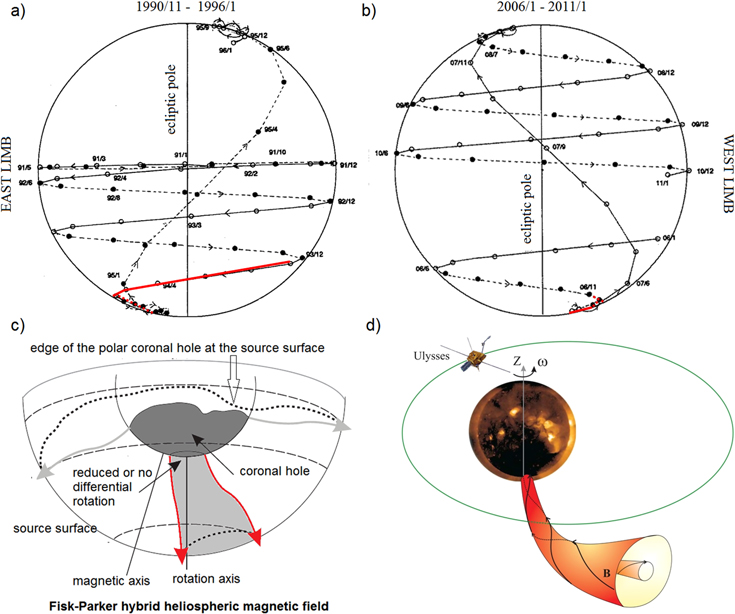
Figure 1. Projection of the Ulysses path on the solar surface for the (a) first and (b) third solar orbit, according to Heliospheric Trajectory Book 3. The projection during the period of interest is shown by the red curve. (c) The conic-like light-gray region separating the Fisk-type and pure Parker magnetic field has a border shown by red arrows, representing a current sheet. Adapted from Burger et al. (2008). (d) Ulysses schematic trajectory while crossing the conic-like current sheet at high heliolatitudes.
Download figure:
Standard image High-resolution imageThe existence of conic-like magnetic separators in high latitudes was foreseen by Burger et al. (2008) in their version of the Fisk–Parker hybrid field model (Fisk 1996), which supposes that a region bordering the pure Parker magnetic field and the hybrid field should occur at high heliolatitudes. However, it has not been confirmed observationally. The model of Burger et al. (2008) takes into account differential photospheric rotation and rigid coronal hole rotation, which produces a separate conic polar region inside a coronal hole. Magnetic field footpoint motion occurs only through diffusive reconnection in that region (Burger et al. 2008). If so, the border of the region should be a current sheet, as there are conditions favorable for its formation in the solar corona (Stevenson et al. 2015). Edges of coronal holes also represent current sheets with the confirmed effect of magnetic reconnection on the boundary between open and closed magnetic flux (Edmondson et al. 2009; Higginson et al. 2016). The question is, how stable are such conic-like current sheets are, and how far from the Sun can they be observed in situ?
The schematic representation of field lines according to Burger and coworkers' modification of the Fisk–Parker hybrid field model is shown in Figure 1(c), adapted from Burger et al. (2008). The light-gray conic Fisk–Burger region with no differential rotation is located inside the dark-gray coronal hole. The real shape of the current sheet, bordering it from Parker-like solar wind, may be more complicated over the Alfvén radius (being, for example, spiral-like), but it cannot be distinguished by a single spacecraft. Figure 1(d) represents the continuation of Figure 1(c) into the solar wind and shows Ulysses, crossing a conic-like current sheet inside the coronal hole flow (not to scale). As we will show below, the CCS is a magnetic tornado-like formation and its internal fine structure may be rather complicated, as secondary embedded current sheets with a varying magnetic field direction occur inside the main CCS, but the key feature of the CCS is the solar wind plasma of low velocity and high beta.
A high-latitude large coronal hole that contained a CCS was observed for several months in 1994, being much smaller in the beginning of 2007 February and fully developed just by the end of the month, according to Yohkoh Soft X-ray Telescope and SOHO EIT images (see http://ylstone.physics.montana.edu/ylegacy/ and http://sohowww.nascom.nasa.gov/data/archive/index_ssa.html or http://www.ias.u-psud.fr/eit/movies/). The image used for the sketch in Figure 1(d) is from Yohkoh, taken on 1994 February 6. It should be noted again that a single, point-like crossing of a high-latitude current sheet by Ulysses does not allow us to distinguish between the conic and cylindrical form. However, as we will show below, all typical signatures of tube-like current sheets can be observed in situ.
2. Observations of High-latitude Current Sheets
2.1. Multiple Crossings of the CCS in 1994
Unusually sharp variations in the solar wind speed, temperature, density, and IMF were detected several times during the first Ulysses flyby in the south polar heliosphere with a quasi-periodicity of about 1 month during a prolonged period from 1994 January 17 to November 8. Key plasma and IMF parameters observed by Ulysses are plotted in Figures 2(a) and (b) with daily resolution. The horizontal axis in Figure 2(a) is for a heliolatitude, while the longitude varies from 93° to 234° and the heliocentric distance changes from 3.75 to 1.9 au. The Ulysses position closest to the pole is indicated by the arrow in Figure 2(a).
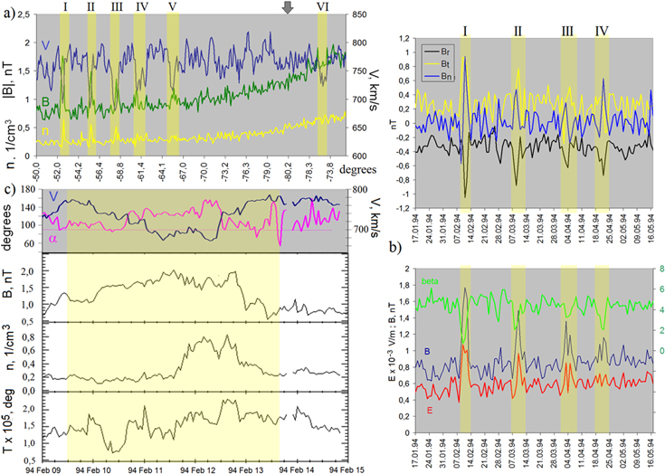
Figure 2. Signatures of a long-lived conic/cylindrical current sheet (CCS) observed by Ulysses at high heliolatitudes during its passage far above the ecliptic plane in 1994. (a) Quasi-periodical decreases in the solar wind speed V and simultaneous increases in density n and the IMF strength B. Daily averages. Periods of crossings of the rotating CCS are indicated by yellow stripes. (b) From top to bottom: the three IMF components in the RTN coordinate system compared to the plasma beta, B and the electric field, E for crossings I–IV indicated in (a). Daily averages. (c) From top to bottom: V and the angle between V and the IMF direction (α), B, n, and the temperature T for the first crossing as seen from hourly Ulysses data.
Download figure:
Standard image High-resolution imageThe sharp changes in solar wind plasma and interplanetary magnetic field (IMF) parameters indicated by yellow stripes in Figure 2(a) are characteristic for crossings of large-scale structures with neutral lines that carry the electric current and possess not a simple, planar form, but a conic or cylindrical shape; in other words, such features are quite typical for CCSs (Zelenyi & Milovanov 1992; Kocharovsky et al. 2009; Popoudin et al. 2012). Inside the CCSs, the solar wind speed V decreases sharply in the background of the fast solar wind typical for open magnetic field lines at high latitudes in solar minima.
During the entire period shown in Figure 2(a), a coronal hole was well formed in the polar region, and the corresponding flow was characterized by a V mean value of 762.4 km s−1 with a standard deviation of 24.5 km s−1 as measured by Ulysses. However, during the CCS crossings V experienced a dramatic drop below 700 km s−1. At the same time, the solar wind density n and the IMF strength B both demonstrated significant increases, as seen in Figure 2.
CCS crossings I–V occurred with a quasi-periodicity of about 1 month, which corresponds to periods of rotation of the Sun in high latitudes. Both plasma and IMF signatures of CCSs become unclear if one analyzes the low-resolution data closer to the South Pole; therefore, we do not indicate the following crossings in Figure 2, although one can find them from the analysis of hourly resolution data. The detailed analysis shows that CCSs were not detected in highest heliolatitudes above 78° in 1994, but the CCS was crossed again when Ulysses moved further from the pole (Figure 2(a), crossing VI).
The IMF and plasma features discussed above could hypothetically be attributed to crossings of the HCS, but there was no corresponding IMF sector change. Even if one tried to interpret the features as crossings of the strongly wrapped HCS, then sizes of the hypothetical "wraps," the periodicity of their detection, a striking similarity of the plasma and IMF behavior inside the structures, and the obvious location of the Ulysses spacecraft inside a coronal hole flow altogether would be in disfavor of such a hypothesis. The most probable explanation of the observed quasi-periodicity of the phenomenon is that Ulysses repeatedly crossed the same rotating CCS inclined to the ecliptic plane.
Figure 2(b) shows variations in the IMF components and the electric field perpendicular to the IMF direction (E), identifying CCS crossings. E is computed through calculations of the V component perpendicular to B. The angle α between the instant B direction and V is shown in the upper panel of Figure 2(c). The normal component of the IMF in the RTN coordinate system shown in Figure 2(b) practically plays the role of the IMF component along the tube, because the IMF azimuthal angle at high and middle latitudes is much larger than predicted by the Parker model (Balogh et al. 1995). The analysis of the IMF topology and dominant IMF directions in 1994 was also performed in Forsyth et al. (1995). In other words, the IMF direction is nearly perpendicular to the plasma flow direction, which is predominantly radial, as reflected in α, which is about 90 before and after the crossing of the CCS.
E increases in the typical way for CCSs at edges of the tube (see Popoudin et al. 2012). The plasma beta, which exceeds 4 in the coronal hole flow surrounding the CCS, strongly decreases inside the CCS, showing that the stability of the CCS is governed by the magnetic field, which is quite unusual so far from the Sun.
The first crossing (CCS I) is shown in detail in Figure 2(c). Parameters n and T are generally in antiphase with V, which is in agreement with modeling of CCSs. There is a slight asymmetry in the behavior of the plasma parameters determined by purely topological factors, as the Ulysses spacecraft crossed the CCS not through the central axis, but closer to the periphery. The IMF outside of the tube is directed toward the Sun, but the higher-resolution data analysis reveals a complex system of CCSs with changing direction of the magnetic field embedded in the main CCS (not shown here; see Figures 5 and 6 for details), which reflects the intrinsic feature of all current sheets in the solar wind to be multiscale (Malova et al. 2017).
An instant (local) IMF direction varies significantly during the crossings of these structures and sometimes may be different from and even opposite to the out-of-tube IMF direction for a short time period when the spacecraft is inside an embedded secondary tube (as illustrated in Figure 1(d)). As we will show below for the CCS observed in 2007, this feature may be evident even under low 1-day resolution from sharp changes in α that often turns to more than 90° and back within a short time period while Ulysses crosses the tube (see Figure 4(c) below and compare with Figure 2(c)).
To understand the local topology of the CCS better, one can calculate components of V with regard to the instant (local) IMF direction and find that the magnetic tube edges are oriented nearly perpendicular to the radial direction as shown in the upper panel of Figure 2(c), since α is close to or larger than 90°. As noted before, the V direction at 1–3 au is predominantly radial, as the radial V component exceeds the other two by an order or two. Changes in α from 90° to almost 180° and back across the CCS, shown in the upper panel of Figure 2(c), correspond to the rotation of instant  regarding
  inside the CCS.
Figure 3(a) illustrates the fact of local magnetic field rotation inside the tube, showing a hodogram of V components perpendicular (Vperp) and parallel (Vpar) to the local  direction through the entire structure. The hodograph rotates in a way that suggests a spiral twisting of the magnetic field regarding V. Analogically, if one calculates Bperp and Bpar with regard to the instant V direction, the rotation is obvious between the nearest embedded conic-like current sheets. Figure 3(b) shows the behavior of the IMF components inside the CCS from Figure 2(c), closer to the edge, from 13 UT to 23 UT on 1994 February 10. The left large panel in Figure 3(b) illustrates the IMF rotation in RTN coordinates with 1-minute resolution, and the small upper right panel shows the same with 1 hr resolution to be sure that the rotation is gradual from point to point. The small lower right panel is an analog of Figure 3(a), but calculated for B with regard to V.

Figure 3. (a) Velocity component hodogram. A half circle seen in the hodogram of the V components perpendicular and parallel to the local IMF direction reflects the spiral rotation of the IMF through the CCS from 09:10 UT, 1994 February 09, to 16:00 UT, 1994 February 13. Hourly averages. (b) Hodograms of B that illustrate the rotation of the instant magnetic field inside the CCS. The left panel shows the radial vs. tangential IMF components plotted with 1 minute resolution, and the right panels show the gradual B rotation in the hodogram of the hourly averaged magnetic field components.
Download figure:
Standard image High-resolution imageTherefore, the whole structure is stabilized by the spiral magnetic field, like in the case of magnetic tornadoes (see, e.g., Wedemeyer-Böhm et al. 2012). Summarizing, the high-latitude CCS may be described as a magnetically governed, low-plasma-beta and low-velocity structure observed in the background of the high-speed polar solar wind typical for the solar minimum.
2.2. Ulysses Observations in 2007: A Solitary CCS above the South Pole
In 2007 February, Ulysses detected unprecedented changes in plasma and IMF parameters during its passage over the South Pole (see Figures 4(a)–(c)). An unusual region was crossed by Ulysses inside the solar wind flow from a small developing coronal hole that finally formed at the end of 2007 February. Two current sheets at the edges of the coronal hole are shown by thin arrows in Figure 4(a).

Figure 4. Crossing of the CCS as observed by Ulysses over the South Pole in 2007. (a) The CCS is indicated by the yellow stripe. The solar wind density (yellow), the IMF strength (green), the electric field (red), and the radial IMF component experience a sharp decrease right over the point closest to the South Pole, indicated by the wide arrow. Two thin arrows show the crossing of current sheets representing the borders of a coronal hole, inside which the CCS was observed. (b) The solar wind speed (dark blue) and the plasma beta (light green) are remarkably low during the CCS crossing. (c) Variations in plasma/IMF parameters shown with higher resolution, similar to Figure 2(c). (d) Velocity component hodogram, analogous to Figure 3(a).
Download figure:
Standard image High-resolution imageThe solar wind speed dropped below 400 km s−1 in the background of the typical high-latitude solar wind having values of about 800 km s−1. The plasma beta was as low as 0.5 during the crossing of some structure in the point closest to the South Pole (Figure 2(b)). E shown in Figure 4(a) and α shown in Figure 4(c) varied similarly to the previous case (see Figure 1); however, embedded secondary current sheets were clearly seen under both low and high resolutions from sharp variations in α (Figure 4(c)), the IMF components (Figures 5, 6), and the IMF angles (not shown here; see Neugebauer et al. 2007 for details). The hodogram of the speed components calculated regarding the IMF direction also illustrates the tornado-like behavior of the IMF through the structure (Figure 4(d)). Therefore, the main signatures of the CCS crossing were observed by Ulysses in this particular case too.
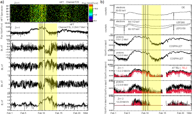
Figure 5. Ulysses measurements of energetic electron and ion flux in 1994 February. The CCS is highlighted by yellow. From top to bottom: (a) energetic ion flux in 32 sectors, Z ≥ 1 ion flux in 0.29–6.7 MeV energy channel; radial, tangential, and normal components of the IMF and its strength; (b) electron counts in two energy channels, proton flux in two energy channels up to 3 MeV, Z ≥ 1 ion flux, proton flux, and Z ≥ 2 ion flux in corresponding energy channels shown in the panel.
Download figure:
Standard image High-resolution image
Figure 6. Analogous to Figure 5. From top to bottom: electron and ion counts in corresponding energy channels, proton flux, and the IMF field variations across the CCS in 2007 February.
Download figure:
Standard image High-resolution imageThe behavior of plasma and IMF parameters shown in Figure 4 is quite characteristic for CCSs and resembles the CCS crossings shown in Figure 2 and discussed above. At the same time, there is an unusual decrease in n instead of its expected increase. Fortunately, this puzzling peculiarity has been noticed in only work dedicated to this unusual event (Neugebauer et al. 2007).
Neugebauer et al. (2007) have interpreted the event as the crossing of a cometary plasma tail. However, the solar wind density should increase inside the cometary tail in the case of the ordinary interaction of a comet with the solar wind owing to conservation of momentum and energy, as mentioned in Neugebauer et al. (2007). Furthermore, both recent observations and simulations do not support the idea that the cometary tail can be traced unambiguously in the solar wind as a separated plasma structure so far from the nucleus (see Reyes-Ruiz et al. 2010; Broiles et al. 2015; Rubin et al. 2015; Volwerk et al. 2016 and references therein). Plasma features that allows one to distinguish the cometary plasma tail from the surrounding solar wind depend on the comet's position, but generally they get masked by the surrounding solar wind as far as ∼0.5 au from the comet, and the cometary tail can be traced further mainly by the presence of cometary ions in the solar wind. Comet McNaught associated with the event was at 0.7 au, while Ulysses was at 2.4 au. As reported in Neugebauer et al. (2007, p. 1263), some weak signatures of the typical plasma tail crossing were observed before the main drop of the parameters, but the subsequent behavior of the parameters associated with a structure identified by us as a CCS was not consistent with theoretical expectations of a cometary plasma tail crossing.
Comparing and combining the obtained results with previous findings, one can suggest that the unusual variations in V, B, and n are due to the prolonged interaction of the CCS with comet McNaught, which approached the South Pole during the period of interest. Hot cometary ions force the solar wind ions out of the tube to maintain the momentum and energy balance, which is observed as the n drop. As reported before, comet McNaught possessed the tail composed of neutral Fe atoms, and there were signatures of the formation of a diamagnetic cavity near the nucleus (Fulle et al. 2007), which could produce the effect of enhanced magnetic tube after the cometary plasma tail interaction with the CCS close to the Sun. Therefore, the discussed event is likely a consequence of the cometary plasma tail disconnection by a current sheet, which is a well-known phenomenon (Niedner & Brandt 1978; Yi et al. 1996). The uniqueness of the event is merely in the form of the current sheet that was interacting with the comet, as current sheets in the solar wind are supposed to be predominantly flat, and CCS–comet interactions have never been investigated before.
2.3. Ulysses Observations of Energetic Particle Enhancements Associated with Crossings of CCSs
The existence of long-lived CCSs in the high-latitude solar wind could shed light on how energetic particles reach high latitudes. Ulysses observations raised the problem of the unusual presence of energetic particles of MeV energies at high heliolatitudes, which is still poorly understood (see, e.g., Smith et al. 2001; Sanderson et al. 2003; Lario et al. 2004; Sanderson 2004; Malandraki et al. 2009). Energetic particles of such energies should propagate mainly along magnetic field lines, but if a source is an active region at low latitudes, it is not clear how they get to high latitudes, being detected there sometimes with a very short time delay with in-ecliptic observations that cannot correspond to particle diffusion across magnetic field lines. Observations of keV–MeV energetic particles in polar regions in quiet times of solar minima are also puzzling.
Malandraki et al. (2009) have shown that the unusual energetic particle events observed in 2006 December were associated with particle propagation along magnetic field lines without crossing them. The finding of CCSs lets us suggest that energetic particles can be produced by magnetic reconnection either at the edges of a CCS in the solar corona or directly in the solar wind. In the case of coexistence of a high-latitude CCS and an active region at lower latitudes, a multiple wave-like interchange reconnection initiated in the active region and propagating to the pole can provide easy access of solar energetic particles to the CCS (see also Edmondson et al. 2009; Higginson et al. 2016). Reconnection-driven polar jets (Szente et al. 2017) that occur at the borders of a CCS can be potential sources of accelerated particles during quiet times as well.
Indeed, energetic particle flux enhancements were observed by Ulysses at edges of CCSs in both 1994 and 2007 (Figures 5 and 6). In 1994 this effect was clearer, perhaps because the equipment worked better than in 2007 and the time-intensity profiles were not so noisy.
Figure 5(a) shows energetic particle flux measurements by COSPIN (COsmic Ray and Solar Particle INvestigation) presented from the Low Energy Telescope, High Flux Telescope (HFT), and Anisotropy Telescope. Electron counts are from the Low-Energy Magnetic/Foil Spectrometers (LEMS DE and LEFS) as parts of the Ulysses heliosphere instrument for spectra, composition, and anisotropy at low energies (HI-SCALE). The description of corresponding instruments can be found at http://www.cosmos.esa.int/web/ulysses/instruments. The IMF components shown in the bottom panels of Figures 5(a) and 6 vary in a way typical for crossings of current sheets embedded in the main CCS. The three clearest crossings at one side of the CCS are shown in Figure 5(a) to highlight corresponding local enhancements in the ion flux observed in the 0.29–6.7 MeV channel (HFT) in the background of a larger-scale energetic particle flux enhancement with a maximum outside the edge of the CCS, which may be a signature of the combination of magnetic reconnection ongoing inside the tube and solar energetic particle propagation along the borders of the CCS. Similar variations are seen in electron and proton/ion flux in Figure 5(b).
In 2007, local particle acceleration associated with the CCS crossing was clear for ions with energies up to 130 keV, and a larger-scale enhancement near one of the CCS edges was observed for electrons with energies of 40–65 keV and protons possessing energies up to 3 MeV (Figure 5).
3. Evidence for a High-latitude CCS from Reconstructions of the Magnetic Field and Speed to the Source Surface
3.1. Coronal Magnetic Field Reconstructions
The occurrence of the CCS at high heliolatitudes during solar minima can be indirectly confirmed via the reconstruction of the 3D structure of the coronal magnetic field. Magnetic field lines shown in Figure 7 are calculated from the Wilcox Solar Observatory (WSO) daily synoptic maps (magnetograms), using an analog of the potential field source surface model, as described in Obridko et al. (2000). Magnetic field lines are reconstructed from the photosphere to the source surface.
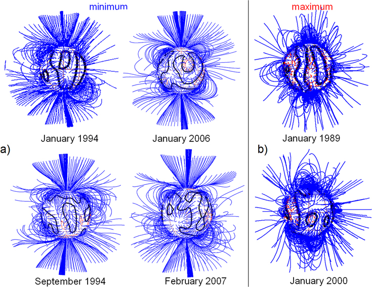
Figure 7. Configurations of coronal magnetic field lines based on extrapolation of photospheric magnetic fields to the source surface. (a) Solar minima; (b) solar maxima.
Download figure:
Standard image High-resolution imageFigure 7(a) clearly demonstrates long-lived CCS-like structures occurring in polar regions. Interestingly, in the beginning of 1994, the structure over the South Pole is declined from the rotation axis much more strongly than in 2006–2007, which is in accordance with in situ observations. Figure 7(b) is given to illustrate the absence of such structures during solar maxima, as found from the analysis of the whole available WSO database.
The obtained observational results are in agreement with solar measurements and confirm the idea that polar coronal holes are not simple monopolar structures, but rather complicated formations that may contain regions with closed magnetic field lines (Chertok et al. 2002; Obridko & Shelting 2011). Therefore, we confirm that the complexity of the polar coronal region seen in magnetic field measurements is reflected in the solar wind in situ observations. The CCS in 2007 was observed in the solar wind that could not be attributed to a well-formed coronal hole; however, the existence of open field lines assured the high-speed outflow from the polar region for a prolonged time in 2007 February. The difference between two types of the fast solar wind from high and mid-heliolatitudes associated with coronal holes has also been discussed in Bisi et al. (2007) in terms of comparisons of Ulysses measurements and IPS data.
3.2. Isolated Regions of High-latitude Slow Solar Wind Observed through IPS Measurements
Conic-like magnetic structures restored in the coronal magnetic field at high latitudes can be compared with corresponding solar wind speed maps, as shown, for example, in Figure 2 of Tokumaru et al. (2012). IPS measurements at the Institute for Space-Earth Environmental Research (ISEE) at Nagoya University enable the determination of the global distribution of the solar wind speed (Tokumaru et al. 2010). Figure 8 shows synoptic source surface maps of solar wind speeds derived from ISEE IPS measurements for 1994 and 2007, corresponding to periods of CCS observations in Cycle 22/23 and 23/24 minima, respectively.
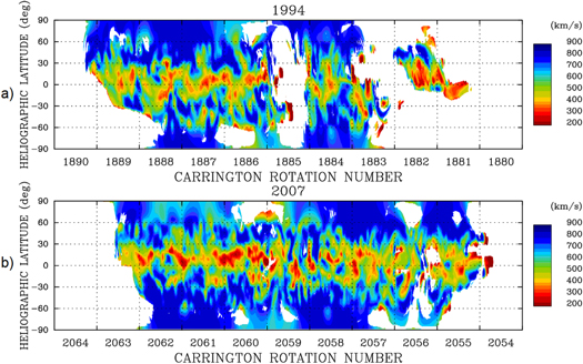
Figure 8. Synoptic source surface maps of solar wind speeds derived from ISEE IPS observations for (a) 1994 and (b) 2007. The abscissa and ordinate at these maps are the Carrington rotation (longitude) and the heliographic latitude, respectively. Note that the Carrington rotation number increases from right to left.
Download figure:
Standard image High-resolution imageAs shown in Figure 8, the fast (700–800 km s−1) solar wind dominates in high- to mid-latitude regions of the heliosphere, and a low-latitude region is associated with the slow (300–400 km s−1) solar wind. The wavy pattern of the low-latitude slow solar wind generally follows the magnetic neutral line on the source surface, which approximately corresponds to the HCS, although their disalignment sometimes leads to the appearance of rapidly diverging open field lines rooted in the vicinity of active regions (Kojima et al. 1999), which may in turn lead to the formation of conic-like current sheets near the ecliptic plane.
The important feature seen in Figure 8 is that isolated regions of relatively slow wind colored blue, green, and yellow occur from high to mid-latitudes, surrounded by the fast wind (dark blue). Some of those slow-wind regions embedded in high-latitude fast solar wind rapidly evolve with time and can be interpreted as transient structures, but some of them are observed repeatedly in several consecutive rotations, suggesting that they correspond to a long-lived quasi-stationary structure with a significantly decreased speed, as discussed in Tokumaru et al. (2017).
Summarizing, reconstructions of solar wind speed profiles and magnetic fields closer to the Sun reveal the existence of specific regions located inside polar coronal holes or within areas of open magnetic field lines. These regions are characterized by the conic-like shape of the IMF and the dramatically decreased speed as observed in solar minima.
4. Modeling of CCSs
The existence of CCSs at high heliolatitudes was suggested by Burger et al. (2008), as the proposed model of the heliospheric magnetic field supposed the formation of a conic-like magnetic separator inside a polar coronal hole. At the same time, there have not been attempts to build the model of a CCS in the high-latitude solar wind. Below, we will illustrate that key features of a CCS can be estimated analytically. The biggest problem with building an analytical MHD model of the CCS is in the loss of alignment of  and
and  further from the Sun, as known from observations. For example, the angle between
  and
and  (α) measured by Ulysses at ∼2.5 au was larger than 90° (see Figures 2 and 4). Therefore, we will create two models, one that can be applied to the distances where α is rather small to describe variations of key CCS characteristics with distance, and another that can be used to estimate variations of parameters inside the CCS at distances where α is significant and the width of the CCS can be considered as constant.
First, we will build a simple stationary one-fluid MHD model that would be able to describe a CCS qualitatively and demonstrate that such structures can exist in the solar wind. Let us consider a cylinder along the Z direction in the cylindrical coordinate system  with the center in the center of the Sun (see Figure 9(a)).
  = Br
= Br r + Bφ
 φ + Bz
 z, where
  r,
r,  φ,
φ,  z are directing vectors. Br, Bφ, Bz are the radial, toroidal, and vertical components of
  , correspondingly. The three components of the velocity
  , the current density
  , and the electric field
  are defined analogically.

Figure 9. Modeling of the CCS closer to the Sun, where V and B are approximately parallel to each other. (a) Coordinate system. (b) Width of the CCS vs. distance from the Sun. (c)–(e) Solar wind speed, density, and plasma beta with respect to the distance from the center of the CCS calculated at 100 solar radii.
Download figure:
Standard image High-resolution imageThe pressure P, the plasma temperature T, and the concentration n are bounded by the state equation:

The plasma equilibrium is described by the equations


Here ρ is the plasma density, φ denotes the electric potential (EP), and the polytrophic index γ = 5/3. The model is applicable to distances, where Z ≫ 1 R⊙ (R⊙ is the solar radius), and the angle between  and
and  is lesser than 30°. The boundary conditions are taken from Kislov et al. (2015), but the differential rotation of the photosphere is not considered here for simplification.
The model describes the CCS with a boundary representing a neutral line. The structure linearly expands with distance from the Sun as shown in Figure 9(b). L is the CCS width shown in Figure 9(a), and Z is the distance from the center of the Sun. The plasma density and the IMF strength along Z decrease quadratically, and V almost does not change. The azimuthal magnetic field decreases linearly with distance from the Sun.
One can derive the equations, using methods shown in Kislov et al. (2015), and estimate the behavior of the IMF and plasma parameters across the CCS at a certain distance from the Sun (Figures 9(c)–(e)). Profiles of parameters plotted in Figures 9(c)–(e) are calculated at 100 R⊙ and show general features of CCSs in the solar wind, i.e., the decreased speed and low plasma beta, as well as the increased solar wind density. The secondary maxima in the profile of n gradually disappear by 1.5 au, and the density has one maximum at the axis of the CCS.
Now we can build the second model that provides detailed information on instant variations of the IMF and plasma parameters inside the CCS, such as the IMF components, the solar wind speed and its components, the electric field, the temperature and density, and the plasma beta in the case of nonaligned  and
and  , i.e., at 2–3 au. We will employ here Equations (7)–(8) but vary the symmetry of the model. Observations show that the Z-component of V is dominant farther from the Sun (Z in Figure 9 corresponds to R in the RTN coordinate system) and B is almost perpendicular to it at 2–3 au, where Ulysses crossed the CCSs, so we will choose the Z-symmetry case.
The translational symmetry allows us to reduce the equations of continuity and nondivergence of the magnetic field to identities


where A is the vertical projection of the IMF vector potential, and Γ is the vertical projection of the speed, which also has the meaning of circulation of speed in the plane perpendicular to Z, so let us call Γ simply "circulation." Expressions (9)–(12) allow us to reduce a part of projections (6) to the view of [∇a, ∇b] = 0; hence,

One can find from projections of Equation (6) onto Z that


where f is determined by boundary conditions, Bn, vn are projections of the IMF vector and V in the plane normal to Z, and α is the mass download of magnetic field lines that can be determined through f as follows:

Here α has a dimension of square root of the density.
If one denotes the EP as ψ and employs Equation (13), the condition of equipotentiality of magnetic field lines can be found:

where F is determined by the boundary conditions.
Finally, one can obtain the radial electric field as follows:

here and below B is the module of the magnetic field without taking Bz into account.
The translational symmetry suggests that Ez = 0. As follows from Equation (17), the electric and magnetic fields are perpendicular. Three consequences of Newton's second law (Equation (2)) can be expressed as follows:


Here H denotes the mass density of enthalpy. Equation (19) is the result of projection along Z, Equation (20) the result of projection along Bn, and Equation (21) the result of projection across Bn and Z.
Equations (19)–(21) can be simplified since we describe a symmetric conic or cylindrical structure. Let us simplify the case to a 1D model with both translational and axial symmetry. Also, the pressure and enthalpy in Equations (20)–(21) can be neglected, as the bulk speed of the solar wind exceeds the thermal speed. Finally, we do not pay attention to effects at the edges of the CCS, considering only its internal structure. Mathematically, this means that the vector potential is a monotonic function, and variables that determine the integrals in Equations (19)–(20) can be considered biunique functions. Additionally, the axis of symmetry of the CCS coincides with the axis of rotation of the Sun. Therefore, one can find that


Taking into account Equations (22)–(24), system (19)–(21) can be presented as follows:


Employing Equation (24), one can add Equation (14) to Equations (25)–(27):

EP Ψ and Γ are also single-valued functions of A.
As follows from Equations (26)–(27),

where Bφ 0(A) should be determined. One can find from Equations (10) and (28) an expression for the vector potential as follows:

It is supposed in Equation (30) that A = 0 at the axis of rotation. Equations (18) and (25)–(28) allow us to find all nonzero plasma parameters in the CCS. Functions of vector potential are supposed to be known.
One can find expressions for Z-projections of V and B:


Now we can select boundary conditions. Equations (25), (26), and (28)–(32) are algebraic and so simple that the setting of the boundary conditions for most functions is equal to finding ready solutions. As mentioned above, the model does not work closer to the Sun, but taking into account the previous model and observations, we suppose that key features of angle distributions of plasma parameters remain the same, and the functions of vector potential have the same view as in the solar atmosphere. Since the conic/cylindrical structure is formed in the solar atmosphere, let us treat the CCS as a plasma ejection in terms of the peaking density inside the structure (36). The azimuthal magnetic field, electric field (35), and vector potential (33) are determined by the unipolar generation occurring as a result of the rotation of the conductive foot of the CCS in the dipole solar magnetic field (38). Also, we will take into account the differential rotation of the solar atmosphere (37). Z-projection of  has the form of Equation (39) and the maximum near the pole.
The boundary conditions are as follows:


θ is the angle between the pole and a selected direction. α can be found from Equation (28), and the temperature can be found from the supposition on the adiabatic plasma outflow. Bz and vz are as follows:


The final solutions of Equations (25), (26), and (28)–(32) can be obtained through Equations (33)–(39).
The model cannot be used at distances below the solar radius. It cannot be applied close to the edges of the CCS either because 4πα2–ρ in Equations (30) and (31) equals 0 at the edges.
The obtained solutions for various parameters inside the CCS are shown in Figure 10. Zero corresponds to the axis of symmetry.
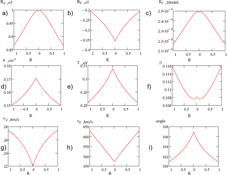
Figure 10. Modeling of the CCS farther from the Sun, where V and B are approximately perpendicular to each other. The dependence of plasma/IMF parameters inside the CCS with respect to the distance from the axis of symmetry (R is in solar radii). (a) Bφ, the azimuthal magnetic field; (b) Bz, the magnetic field along the axis of symmetry; (c) Er, the electric field; (d) n, the plasma density; (e) T, the plasma temperature; (f) β, the plasma beta; (g) vφ, the azimuthal speed; (h) vz, the speed parallel to Z; (i) the angle between V and B.
Download figure:
Standard image High-resolution imageLet us discuss below some features that may induce questions. Bz is the IMF component along the axis of the CCS, and Bφ (Figure 10(a)), which is the azimuthal component, is one order larger than Bz (Figure 10(b)). The radial component is zero owing to the axial and translational symmetry. In reality, the structure may not possess these features, being bounded, so the radial component may exist. The azimuthal magnetic field chosen for the boundary conditions is nonzero near the CCS axis, which may lead to the occurrence of the axial electric current (which indeed was seen under high resolution). The profiles of n and T (Figures 10(a) and (e)) are similar because the solar wind polytrophic index is larger than 1 and equals 5/3 as shown in Khabarova & Obridko (2012).
A small maximum in the center of the plasma beta profile (Figure 10(f)) is due to the slowdown in the growth of the main component of the IMF, which is characteristic for axisymmetric plasma structures like pinches. The plasma beta growth that occurs farther from the center is determined by the slower change in the azimuthal magnetic field. The existence of vz (Figure 10(h)) is explained by the drift in the largest components of the IMF and electric field, i.e., Bφ and Er. The appearance of nonzero Bz leads to the plasma drift in the azimuthal direction. Since magnetic field lines are supposed to be embedded into the plasma (6), the existence of Bz produces twisting of the field of velocities and reduces the difference between the parallel and azimuthal components of the speed. As both Bz and Er have maxima near the axis, the effect of the decreased vz is maximal there.
The obtained results satisfactorily explain qualitative features of observed polar current sheets. As mentioned above, 4πα2–ρ in Equations (30) and (31) equals 0 at the edges of the CCS. The physical meaning of this combination is the equality of the Alfvénic vA and azimuthal vφ speeds. According to the model, vA > vφ inside the CCS; therefore, one can suggest that the physical boundary of the CCS represents the Alfvén boundary.
Figure 11(a) shows computed Alfvén and azimuthal speeds for distances from the CCS axis larger than shown in Figure 10. There is a point at which both speeds equal that corresponding to the Alfvén boundary at the boundary of the tube. The approximate width of the entire structure is 16.2 solar radii, which corresponds to observations very well. It should be noted that the modeled width does not change with distance from the Sun owing to the translational symmetry; however, this is surprisingly in accordance with observations, as the crossings of the CCS in 1994 at different distances from the Sun showed approximately the same width of the structure, so we can conclude that the CCS seems to be tube-like and stable at long distances from the Sun, and our simple MHD model can illustrate the key CCS features adequately.

Figure 11. Alfvén (blue) and azimuthal (red) speeds inside and outside the CCS. (a) Modeling; (b), (c) Ulysses observations in 1994 and 2007, respectively.
Download figure:
Standard image High-resolution image
Figures 11(b) and (c) show vA and vφ calculated for the CCS crossings in 1994 and 2007, respectively. A short-time increase in vφ in the center of the CCS in 1994 may be due to the occurrence of the electric current along the main axis, as discussed above, but generally the observations are well consistent with theoretical predictions.
5. Discussion and Conclusions
We report observations of quasi-stable cylindrical/CCSs with the significantly decreased speed and very low plasma beta at high heliolatitudes during Ulysses passages over the South Pole in the two solar minima (1994 and 2007). The widths of such structures are several times less than the typical width of coronal holes. The modeling shows that the CCS boundary may represent the Alfvén boundary.
The Ulysses plasma and magnetic observations cannot correspond to the HCS crossing, because the found structures are located inside flows from high-latitude coronal holes. The observed structures cannot be jets or plums either (DeForest et al. 2001; Nisticò et al. 2015), as lifetimes of those smaller-scale structures are too short in comparison with lifetimes of CCSs, which are so stable that they can be observed for several months. And, finally, the structures are governed by the magnetic field and have signatures of magnetic tornadoes.
The CCS was declined from the South Pole in 1994, and Ulysses crossed it several times owing to rotation of the structure with a period that supposes corotation of the CCS with the Sun at high latitudes, i.e., the Alfvén radius may be much farther from the Sun over the poles than in the ecliptic plane. The CCS was almost aligned with the rotational axis in 2007, and Ulysses crossed the structure just one time.
The approximate position of the CCS in the corona is in good agreement with tracing the solar magnetic field lines up to the source surface for the corresponding periods. Synoptic source surface maps of the solar wind speed also confirm the occurrence of long-lived regions of slow solar wind embedded in the high-speed solar wind at high latitudes during solar minima.
In 2007, the CCS interacted with comet McNaught right over the pole. As a result, plasma features of the CCS were dramatically highlighted by the interaction. This is the first report on the interaction of a comet with a CCS. We found that such interactions may reveal both structures, allowing their detection at several au. Interestingly, exactly the same variations in plasma parameters were observed by Ulysses at lower heliolatitudes in 1996 inside the high-speed coronal hole flow and associated with cometary ions as well (Gloeckler et al. 2000). In previous studies, the event was called the "density hole" and supposed to be a clear plasma structure, without any mentioning of the comet (Riley et al. 1998). In that particular case the distance between comet Hyakutake's nucleus and Ulysses was 3.4 au, which is even larger than in the above-discussed case of comet NcNaught, which again raises some questions about the idea of pure crossing of the cometary plasma tail, as the detection of cometary ions is not yet evidence for the presence of a well-formed tail recognizable in the background of the solar wind.
Our finding allows us to solve this puzzle and conclude that it also was the case of the comet–CCS interaction rather than an ordinary comet plasma tail crossing. During the comet–CCS interaction, cometary ions channel into the CCS, push cold solar wind ions out of the tube, and form a specific profile of the isolated low-speed CCS governed, as usual, by the magnetic field, but characterized by the decreased solar wind plasma density (which is increased inside ordinary CCSs). Although interactions of comets with current sheets have been known for a long time, even most advanced simulations of disconnection events have been performed only under the assumption of the planar geometry of discontinuities that trigger disconnections, including the HCS–comet interactions (Jia et al. 2007). The occurrence of stable current sheets possessing conic or tube-like form has never been suggested; therefore, the finding allows us to revisit some previous observations of disconnection events and opens possibilities for the development of a new model of interactions of comets with nonplanar current sheets in the solar wind.
Observations of energetic particle flux enhancements at edges of CCSs can solve, at least partially, the problem of observations of energetic particles at high heliolatitude. The CCS represents both a source of local particle acceleration via magnetic reconnection in the solar wind and a magnetic channel for energetic particles accelerated at the Sun.
The existence of CCSs with slower speed and increased density in the polar heliosphere might influence the assessment of ionization rates of interstellar particles observed close to the Sun. If CCSs exist for several months, they can significantly change bulk properties of the solar plasma at high latitudes and consequently influence observed fluxes of such heliospheric particles as interstellar neutral (ISN) gas atoms, energetic neutral atoms (ENAs), and interstellar pickup ions (PUIs). Furthermore, the occurrence of CCSs impacts the distribution of the solar wind as a function of heliolatitude and should be taken into account for the correct interpretation of full-sky maps of hydrogen and helium helioglow in the heliosphere (e.g., Ajello 1978; Broadfoot & Kumar 1978; Lallement et al. 1985, 2010). The ionization reactions most affecting the solar wind conditions are the charge exchange with solar wind particles and electron impact ionization (e.g., Bzowski et al. 2013a, 2013b). As discussed by Sokół et al. (2016), the flux of ISN gas and PUIs detected in the ecliptic plane can be significantly modulated by solar wind conditions out of the ecliptic plane because ISN gas particles enter the heliosphere at various latitudes, propagate through it at mid- and high latitudes, and reach the ecliptic plane at closer distances to the Sun owing to gravitational focusing (see also Figure 12 in Kubiak et al. 2014 for the reference to the distribution of ISN particle positions entering the source region).
The understanding of spatial plasma variations in the polar solar wind is also essential for the study of ENA survival probabilities (Bzowski 2008), such as observations of hydrogen ENAs by the Interstellar Boundary Explorer (IBEX) mission (McComas et al. 2009). IBEX observes the hydrogen ENA fluxes in the form of full-sky maps (McComas et al. 2012, 2014). The increase in the solar wind density and simultaneous decrease in the solar wind speed at high latitudes may influence the assessment of the survival probabilities of ENA flux, as discussed in Appendix B in McComas et al. (2012, 2014). The existence of long-lived CCSs in the polar regions during the solar minimum may also affect the interpretation of the observed ENA flux from the polar caps (e.g., Reisenfeld et al. 2016). Preliminary results show that particles both with low energies (tens of eV) and detected close to the downward axis of the ISN gas flow may be seriously affected by the presence of such structures. Therefore, a possible influence of the conic solar wind plasma structures on propagation of heliospheric particles requires a further careful modeling and checking with available observations.
Summarizing, the finding of high-latitude CCSs in the heliosphere in the solar minima allows the development of studies in the following directions:
- 1.The identification of similar structures from Ulysses measurements over the North Pole, as well at middle and low latitudes during other phases of the solar cycle, which has not been performed yet, since the CCS crossings over the South Pole were more evident.
- 2.The identification of CCSs from IPS data and heliospheric white-light imagery (SMEI, heliospheric imagers on board STEREO-A and STEREO-B) and comparisons with solar magnetic field observations.
- 3.The analysis of the possible impact of CCSs on the spatial and temporal distribution of heliospheric particles, including applications to IBEX observations.
- 4.Understanding of propagation and acceleration of energetic particles observed at high heliolatitudes.
- 5.Modeling of CCSs in the solar wind (both numerical and analytical).
- 6.Modeling of CCS–comet interactions.
None of the above-listed tasks have been completed. Two CCS models presented above are just the first step in theoretical studies of these structures in the polar solar wind.
The discovery of the cylindrical/CCS over the solar pole in the solar minima may be considered as a support for the Burger et al. (2008) model that supposes the occurrence of a separated conic region inside the polar coronal hole. It should be noted that similar tornado-like structures are observed in the terrestrial magnetosphere (Keiling et al. 2012), which may be counted in favor of universality of formation of high-latitude CCSs, occurring in different plasmas as a result of rotation of space objects. It is quite possible to find such structures over the Jovian poles.
Ulysses data were taken from the official Goddard Space Flight Center OMNIweb plus Web site: http://omniweb.gsfc.nasa.gov. We are grateful to the WSO team for providing magnetograms (http://wso.stanford.edu). O.V.K. was supported by RFBR grant no. 16-02-00479 and by RFBR grant no. 17-02-01328. H.V.M. was supported by RFBR grant no. 16-02-00479 and no. 16-52-16009 NCNILa. J.M.S. acknowledges the support by grant no. 2015-19-B-ST9-01328 from the National Science Center, Poland.
We are grateful to Bernard Jackson and Mario Bisi for inviting the authors to attend the IPS workshop 2016, which allowed O.V.K., J.M.S., and M.T. to correlate works on seeking the CCSs conducted separately at different institutions.