


ABSTRACT
Assessing the interaction between solar acoustic waves and sunspots is a scattering problem. The scattering matrix elements are the most commonly used measured quantities to describe scattering problems. We use the wavefunctions of scattered waves of NOAAs 11084 and 11092 measured in the previous study to compute the scattering matrix elements, with plane waves as the basis. The measured scattered wavefunction is from the incident wave of radial order n to the wave of another radial order n', for  . For a time-independent sunspot, there is no mode mixing between different frequencies. An incident mode is scattered into various modes with different wavenumbers but the same frequency. Working in the frequency domain, we have the individual incident plane-wave mode, which is scattered into various plane-wave modes with the same frequency. This allows us to compute the scattering matrix element between two plane-wave modes for each frequency. Each scattering matrix element is a complex number, representing the transition from the incident mode to another mode. The amplitudes of diagonal elements are larger than those of the off-diagonal elements. The amplitude and phase of the off-diagonal elements are detectable only for
  and
and  , where
  is the change in the transverse component of the wavenumber and Δk = 0.035 rad Mm−1.
Export citation and abstract BibTeX RIS
1. INTRODUCTION
One of the major subjects in helioseismology is the use of solar acoustic waves to probe sunspots. Several data analysis methods have been developed for this purpose, such as the ring-diagram analysis (Hill 1988; Rajaguru et al. 2001; Nicholas et al. 2004; Bogart et al. 2008; Baldner et al. 2013; Jain et al. 2015), Hankel analysis (Braun et al. 1987; Bogdan et al. 1993; Braun 1995; Chen et al. 1996; Sun et al. 1997; Couvidat 2014), time–distance analysis (Duvall et al. 1993, 1996; Kosovichev 1996; Chou et al. 2000, 2009a, 2009b, 2009c; Kosovichev et al. 2000; Zhao et al. 2010, 2011b), and acoustic imaging (or acoustic holography; Chang et al. 1997; Chen et al. 1998; Braun & Lindsey 1999, 2000; Chou et al. 1999; Chou 2000; Lindsey & Braun 2000; Sun et al. 2002).
A different method has been developed recently. Cameron et al. (2008) calculated the cross correlation between a line-averaged Doppler signal outside a sunspot and the signal at the points in and around the sunspot for f-mode waves. The cross-correlation function, as a function of space and time, represents the propagation of an acoustic wave packet starting from the line through the sunspot. However, the cross-correlation function is not the wavefunction of the radial velocity of solar acoustic waves. The wavefunction of radial velocity is the radial component of velocity vector, which is the solution of the wave equation for solar acoustic waves. Zhao et al. (2011a) applied a deconvolution scheme on the cross-correlation function to remove the Fourier amplitude of the signal at the reference line, where the incident wave starts, and keep only its phase in the the cross-correlation function in order to obtain the wavefunctions of radial velocity of solar acoustic waves scattered by a sunspot for each radial order. Zhao & Chou (2013) further improved the method and were able to measure the scattered wavefunctions between adjacent radial orders. The scattered wavefunction is defined as follows: For an incident wave propagating toward a sunspot, after interacting with the sunspot, the wave is modified around the sunspot. The modified wave can be expressed as the sum of the incident wave and the scattered wave. The scattered wave satisfies an inhomogeneous wave equation. The inhomogeneous term, called the source term, is responsible for the generation of the scattered wave (Zhao et al. 2011a). Yang et al. (2012) set up a phenomenological model to describe this source term, and used the measured scattered wavefunctions to determine the parameters of the model by iterative fits up to a high-order Born approximation. Chou et al. (2012) used the measured total wavefunction (the sum of the incident and scattered wavefunctions) around the sunspot to compute a one-dimensional hologram, and demonstrated that this hologram could be used to reconstruct the two-dimensional wavefronts on the surface. Zhao & Chou (2016) used the measured scattered wavefunctions to compute the absorption cross section and scattering cross section for each radial order for the interaction between waves and sunspots.
Assessing the interaction between solar acoustic waves and sunspots can be considered a scattering problem. For a scattering problem, the most complete measured information is the scattering matrix. Each element of the scattering matrix is a complex number, representing the transition between two modes, or the conversion from one incident mode to another mode due to the interaction. The discussion of the general theory of the scattering matrix can be found in many physics textbooks (Bjorken & Drell 1964; Schiff 1971). For the interaction of acoustic waves with sunspots, the theory of the scattering matrix has been studied by various authors (Bogdan & Cattaneo 1989; Chou 1994; Fan et al. 1995; Chou et al. 1996; Hindman & Jain 2012). So far no correct measurement of the scattering matrix for the interaction between acoustic waves and sunspots has been reported. Hankel analysis has measured the amplitude change and phase change between an ingoing mode and an outgoing mode. However, these changes are not the amplitude and phase of the individual scattering matrix element. Instead, they are certain combinations of scattering matrix elements, as expressed by Equations (26) and (28) in Braun (1995). This is because the incident wave in Hankel analysis consists of many modes instead of a single mode. The multimode of the incident wave is such that each outgoing mode is a mixture of the scattered signals coming from various ingoing modes, owing to the mode mixing (see also Hindman & Jain 2012). If the mode mixing is negligibly small, the measurement in Hankel analysis can serve as an estimate for the scattering matrix elements. However, the mode mixing is non-negligible and even significant for some modes.
In this study, we devise a method of using a single-mode incident wave to measure the scattering matrix elements. The scattered wavefunctions measured in Zhao & Chou (2013) are the signals scattered from the incident wave of one radial order into the wave of another radial order, because these wavefunctions were measured with the cross correlation between the waves of two radial orders. Since the incident wave belongs to a particular radial order and propagates in a particular direction, each of its temporal Fourier components is a single mode (plane wave). For a time-independent sunspot, there is no mode mixing between different frequencies. Thus each temporal Fourier component of the scattered wave comes from the single-mode incident wave of the same frequency. Expanding the scattered wave of this frequency in terms of different spatial modes gives the scattering matrix elements between this incident mode and various scattered modes. In this study, we use the scattered wavefunctions measured in Zhao & Chou (2013) to compute the amplitude and phase of the scattering matrix elements for the transitions above the noise level.
In Section 2, the general definitions of transition matrix and scattering matrix for a single-mode incident wave are discussed. In Section 3, the method of computing transition matrix elements using the scattered wavefunctions measured in Zhao & Chou (2013) is discussed. Section 4 discusses the methods of determining the amplitude and phase of transition matrix elements. In Section 5, each step of data analysis in computing the transition matrix element from the measured scattered wavefunctions is described and the determination of the amplitude and phase of the measured transition matrix elements is discussed. Section 6 discusses the result of the amplitude and phase of the detectable transition matrix elements. The
2. DEFINITIONS OF TRANSITION MATRIX AND SCATTERING MATRIX
Consider the interaction of the acoustic waves with a sunspot as a scattering problem. An incident wave, represented by the wavefunction of velocity vector  , propagates toward the sunspot, where the superscript i denotes the incident wave. It satisfies the wave equation of the quiet Sun. After interacting with the sunspot, the incident wavefunction
  is modified to
  in and around the sunspot. The difference
  is defined as the scattered wavefunction (Morse & Feshbach 1953; Jackson 1999), where the superscript
  denotes the scattered wave. The scattered wavefunction
  represents the signal generated by the sunspot that is perturbed by the incident wave.
In this section, a general definition for the transition matrix and the scattering matrix is given. First, the formal definition for the transition matrix in the three-dimensional space is discussed. Then its relation to a measurable quantity on the two-dimensional surface, called the "two-dimensional transition matrix," is discussed. The eigenfunctions of velocity (or displacement) vector of solar oscillations in the quiet Sun are orthonormal and form a complete set, denoted as  , where β labels the spatial mode parameters and
  is the corresponding angular frequency. The eigenfunction
  is normalized as

 , where the weighting function
  is the mass density (Unno et al. 1989). Since we are working in a small area, the coordinates
  can be approximated by the Cartesian coordinates
  , where (x, y) are the horizontal directions and z is the vertical (radial) direction, and β labels
  , where n is the radial order, and kx and ky are the horizontal wavenumbers. The frequency
  is connected with
  through the dispersion relation.
Suppose the incident wave is a single mode and its wavefunction is an eigenfunction of the quiet Sun  . If the sunspot is time independent, the interaction with the sunspot would not modify the frequency
  . Since the sunspot has the spatial dependence, the interaction with the sunspot would modify the wavenumber
  . The scattered wavefunction corresponding to this incident wave is denoted as
  , where the subscript α in
  specifies this scattered wave coming from the incident mode α. The spatial part
  is different from the incident mode
  and can be expanded in terms of the complete and orthonormal set of
  as
as

where the expansion coefficient  , a complex number, is called the element of the transition matrix (T-matrix) with the eigenfunctions
  as the basis (Bjorken & Drell 1964; Schiff 1971). It is noted that the T-matrix element is defined in the three-dimensional space. Since the scattered wavefunction
  has the frequency
  , the coefficient
  is nonzero only when the mode β has the same frequency
  . If the T-operator
  is defined as
  , the T-matrix element
  is calculated as
  . The scattering matrix (S-matrix) is the sum of the unity matrix and the T-matrix.
In helioseismology, the three-dimensional distribution of the vector wavefunction  in Equation (1) is unavailable. The observed helioseismic data are the Doppler signals which are the line of sight components of oscillatory velocity on the solar surface. For the modes of interest, the horizontal component is smaller than the radial component on the surface (Unno et al. 1989). Since the data used in this study are near the disk center, the contribution from the radial component is predominant in the observed Doppler signal. The radial component of the velocity is restored by a simple geometric correction, as most of data analysis (e.g., Zhao & Chou 2013). The measured wavefunction used in this study is the radial component of velocity on the solar surface.
If the radial components of  and
and  in Equation (1) are denoted as
  and
and  , respectively, the radial component of Equation (1) is

If Equation (2) is evaluated at the surface  ,
,  on the lhs becomes
  , which is the scattered wavefunction measured on the surface;
  on the rhs at the surface becomes
  , where
  is the radial eigenfunction evaluated at the surface and
  is the two-dimensional orthonormal eigenfunction in the quiet Sun. In our study,
  is the normalized plane wave on the surface, but it can in general be any two-dimensional orthonormal function. The proportional constant of
  is determined by that of
  , which is determined by the normalization of the velocity vector
  . With the notation defined previously, Equation (2) evaluated at the surface can be expressed as

This equation is an expression on the two-dimensional (x, y) plane. It can be viewed as the scattered wavefunction measured on the surface,  , expanded in terms of a set of two-dimensional orthonormal eigenfunctions
  . The expansion coefficient
  , called the "two-dimensional T-matrix element," is calculated by
 on the surface. Thus the T-matrix element
  can be obtained from dividing the measured two-dimensional T-matrix element by
  , which can be calculated with a standard solar model.
3. TRANSITION MATRIX ELEMENTS IN THIS STUDY
The measurement of the scattered wavefunction in Zhao & Chou (2013) does not use a single mode as the incident wave. Instead, the wave packet of a particular radial order n propagating in a particular horizontal direction is used as the incident wave. The scattered wavefunction is measured with the cross correlation between the signal of n and the signal of n', where n' could be equal to or different from n. That is, the measured scattered wavefunction represents the signal converted from the incident wave of n to the scattered wave of n'. Both the incident wave and the scattered wave consist of many modes of different frequencies. Therefore the formulas in Section 2 for the single-mode incident wave cannot be applied directly. Some more processes are needed.
Since the interaction does not change the frequency, part of the energy of an incident mode would be converted into other modes with different wavenumbers but the same frequency. Therefore the scattering problem can be worked in the ω domain for each ω separately. The incident wave of n, denoted as  , is a wave packet propagating in a particular direction on the surface. It consists of many modes of different frequencies propagating in the same horizontal direction, and can be expressed in terms of temporal Fourier series as

where  is the Fourier coefficient and
  is the eigenfunction of the quiet Sun with a radial order n, propagating in the particular horizontal direction. In our study, the incident wave propagates in the y direction. Thus only the modes with kx = 0 can be present in each Fourier component
  in Equation (4). Moreover, from the dispersion relation
  , each frequency corresponds to only one ky for each n. Therefore there is only one mode (
 present in each Fourier component
  .
.
It is noted that each  in Equation (4) does not correspond to a real single mode; instead, it corresponds to one bin in the domain of
  . The size of the bin depends on the spatial size and temporal duration of the data used in the Fourier expansion. In the following discussion, the term "mode" is used for the bin in the domain of
  .
.
Now we come to the scattered waves. The scattered wavefunction from n to n' is denoted as  . It can be expanded in terms of a temporal Fourier series as

where  is the Fourier component. Since the interaction does not cause any cross talk between the modes of different frequencies, each scattered wave
  in Equation (5) comes from the corresponding incident wave
  in Equation (4). Each incident mode
  is converted into the scattered wave, denoted as
  . Thus we have
  . Since the scattered wave
  propagates in multiple directions, it contains many modes with frequency
  and radial order n'. Like Equation (1), the scattered wave
  can be expanded in terms of the eigenfunctions of the quiet Sun with radial order n',
  , and the expansion coefficients are the T-matrix elements. Therefore we arrive at

where  and the expansion coefficient
  is the T-matrix element between the incident mode α of radial order n and the scattered mode β of radial order n'. It is worth emphasizing that this expression is valid only for time-independent sunspots.
Like the discussion leading to Equation (3), we take the radial component of Equation (6) and evaluate it at the surface. The radial component of  evaluated at the surface is denoted as
  , which is the temporal Fourier component of the measured scattered wavefunction
  from n to n' in Zhao & Chou (2013). The index α in
  represents the mode parameters of the incident mode. The radial component of
  evaluated at the surface is denoted as
  , where
  is the radial eigenfunction of n' evaluated at the surface, and
  is the orthonormal horizontal eigenfunction of the quiet Sun. With the notation defined previously, the radial component of Equation (6) evaluated at the surface becomes
The quantity  is the expansion coefficient as
  being expanded in terms of the orthonormal horizontal eigenfunctions of radial order n',
  .
.
Similarly, for the incident wave, the radial component of Equation (4) evaluated at the surface yields
where  is the radial component of the incident wavefunction
  evaluated at the surface and
  is the radial eigenfunction of n evaluated at the surface. The quantity
  is the expansion coefficient as
  being expanded in terms of the horizontal eigenfunctions of radial order n,
  . The function
  is the incident wavefunction measured in Zhao & Chou (2013).
From Equations (7) and (8), the T-matrix element  can be expressed as
where  and
and  can be obtained by expanding the measured wavefunctions
  and
and  in terms of the temporal Fourier series and orthonormal horizontal eigenfunctions, respectively. The quantity
  is called the "two-dimensional T-matrix element." The goal of this study is to determine the complex
  from the measured incident and scattered wavefunctions. From
  , one can obtain the T-matrix matrix element
  with Equation (9). The conversion factor
  can be obtained from the eigenfunctions calculated with a standard solar model.
In this study, the horizontal eigenfunction  is the plane wave in the Cartesian coordinates. Following the setup in Zhao & Chou (2013), the incident wave
  propagates in the y direction. Thus only the modes with the wavenumber
  exist in the expansion of Equation (8), where ky relates to (
 ) through the dispersion relation. Since the frequencies of incident mode α and scattered mode β are the same, the subscripts α and β in frequency ω are dropped hereinafter. If the mode parameters of the incident mode α are
  and the parameters of the scattered mode β are
  , the two-dimensional T-matrix element
  is explicitly expressed as
  for clarity in the following discussion. The condition of equal frequency requires that the incident mode (n, k) and the scattered modes
  correspond to the same frequency ω, where
  and
and  . The two-dimensional T-matrix element is calculated as
where the coefficient of the incident mode  is calculated from the measured incident wavefunction of n by the Fourier transform,

and the coefficient  is calculated from the measured scattered wavefunction of n' by the Fourier transform,
Both  and
and  are complex. The determination of their phase and amplitude will be discussed in the next section.
4. METHOD OF DETERMINING THE AMPLITUDE AND PHASE OF TRANSITION MATRIX ELEMENTS
4.1. Method of Determining the Amplitude and Phase of 

In computing  with Equation (11), first the temporal Fourier transform of the incident wavefunction
  is carried out. Then, for each frequency ω, it is Fourier transformed into the domain of
  . The value of
  is nonzero only at kx = 0. From the dispersion relation, each (
 ) corresponds to one ky, denoted as
  . Each incident mode is labeled by (
 ). Since the Fourier domain of ky is discrete, the value of
  may not be exactly equal to one of the Fourier wavenumbers, which are determined by the spatial size of the data used in computing the Fourier transform; that is,
  may not be exactly located at one of the grid points in the ky domain. Thus the determination of the phase and amplitude of
  requires some added care, the details of which are discussed in the
The  is not at a grid point, the power of
  would spread into all grid points of ky, although
  peaks at the grid point nearest
  . The summation of
  over all grid points of ky equals the power of the mode
  . However, since
  decreases quickly away from
  and noise dominates as ky is far from
  , in practice, we need to sum
  over only the neighboring grid points of
  . The amplitude of this mode
 .
.
The phase determination is a little more complicated if  is not located at the grid point. From the discussion presented in the
  can be computed from a linear interpolation between the phases of
  at two grid points nearest
  . The phase of
  is the linear interpolation evaluated at
  .
.
4.2. Method of Determining the Amplitude and Phase of

Like  , in computing
  with Equation (12), first the temporal Fourier transform of the scattered wavefunction
  is carried out, and then, for each ω, it is Fourier transformed into
  . Each incident mode is scattered not only into different radial orders, but also into different horizontal wavenumbers, while keeping the frequency unchanged. Thus the incident mode (
 ) would be scattered into various modes
  . However, only a few modes around
  are detectable, because the scattered wave propagates predominantly in the y direction, although its wavefronts are curved. The signal of other
  's is not above the noise level. For each (
 ), the value of
  , denoted as
  , is determined by the dispersion relation. For example, for the case of n' = n,
  because
  and kx = 0. The value of
  may not be exactly located at one of the grid points of
  . The amplitude and phase of
  are calculated as those of
  , discussed in Section 4.1.
5. DATA ANALYSIS
5.1. Incident and Scattered Wavefunctions
The incident wavefunction and scattered wavefunction used here are from Zhao & Chou (2013). These wavefunctions are computed from SDO/HMI data, which are 4096 × 4096 full-disk Dopplergrams taken at a rate of one image every 45 s. Two active regions, NOAAs 11084 and 11092, are studied. A time series of 12,402 frames (June 29–July 5, 2010) is used for NOAA 11084 and 12,118 frames (July 31–August 6, 2010) for NOAA 11092. Each of these two active regions has only one sunspot, which is approximately round and changes very little during the period of study (see Figure 1 in Zhao & Chou 2013). Thus the scattering problem here is considered time independent.
The total wavefunction  on the surface around the sunspot is measured using a deconvolution method, and the cross-correlation function computed between the signal averaged over a reference line outside the sunspot and the signal at the points in and around the sunspot on the surface. The line-averaged signal and the point signal are formed by the modes of radial orders n and n', respectively (n' can be equal to or different from n). The signal of radial order n is obtained by applying a ridge filter in the
  domain (Cameron et al. 2008; Zhao et al. 2011a). The same method is applied to the signal of n in the quiet Sun to obtain the incident wavefunction
  . For the case of n' = n, the scattered wavefunction from n to n is
  . For the case of
  , the scattered wavefunction from n to n' is
  . A detailed description of the measurements of scattered wavefunctions is discussed in Zhao et al. (2011a) and Zhao & Chou (2013). As an example, the scattered wavefunctions from n = 4 to n' = 3, 4, 5 are shown in Figure 1. The dimension of each map is
  (400 × 400 pixels). The size of each pixel is
  , or 0.712 Mm. The amplitude of the incident wavefunction on the reference line at t = 0 is set to unity. The animation of measured scattered wavefunctions for different n and n' (
 ) can be found in Zhao & Chou (2013).

Figure 1. Scattered wavefunctions from n = 4 to n' = 3 (left columns), 4 (middle column), 5 (right columns) at three different times (similar to Figure 10 in Zhao & Chou 2013, but with improved data analysis). The dimension of each map is  (400 × 400 pixels). Each pixel is
  , or 0.712 Mm. The red circle indicates the location and size of the penumbra. The incident wave packet starts from the reference line, marked by a red line at y = 0; the sunspot is centered at y = 70 pixels. The amplitude of the incident wave on the reference line at t = 0 is set to unity. The blue square box in panel (a) indicates the area used in computing the Fourier transform in Equations (11) and (12).
Download figure:
Standard image High-resolution image5.2. Dissipation Correction
Both the incident wave and the scattered wave suffer from dissipation. their wave amplitude decreases as they propagate through the Sun. In determining the T-matrix elements, the dissipation effect needs to be corrected because the T-matrix should not contain information of dissipation. In this study, we use the measured dissipation rate of the incident wave in the quiet Sun to correct the dissipation of the scattered wave.
Since dissipation is frequency dependent, the dissipation correction has to be carried out for each frequency. The incident wave propagates only in the y direction. To reduce noise, the incident wavefunction  is averaged over x to obtain
  , which is shown in Figure 2. The wave packet, which starts from the reference line, exists in only a certain region in the (y, t) domain. The upper-left region in Figure 2 has no signal because it corresponds to the spatial region behind the wave packet. There is also no signal in the lower-right corner in Figure 2 because it corresponds to the spatial region ahead of the wave packet; that is, the wave packet has not yet reached this spatial region. The weak residual value in these two regions is noise. Thus we keep only the signals in the region between two red lines in Figure 2 when computing the temporal Fourier transform. Hereinafter, the region with signals is called the signal domain; the region outside the signal domain is called the noise domain. The range of the signal domain is determined with a criterion that the signal is greater than twice the noise level, whose value is computed with an area in the quiet Sun. The value of
  is set to zero in the noise domain in computing the temporal Fourier transform. The boundary between the signal and noise domains is smoothed with a Hann window.

Figure 2. Incident wavefunction averaged over x,  , for n = 2. The region between two red lines is the signal domain, which is used in analysis. The amplitude at y = 0 and t = 0 is set to unity.
Download figure:
Standard image High-resolution imageThe temporal Fourier transform transforms  into
into  . The amplitude
  as a function of
  is shown in Figure 3(a). It should be mentioned that the mask of the noise domain of
  indeed reduces the noise in
  . The distribution of
  versus
  should be smooth, and its fluctuation is believed to be noise. Thus a two-dimensional smoothing in
  is carried out for
  , with a box running mean of 7 × 7 points. The smoothed
  is shown in Figure 3(b). For each ω, the smoothed
  has an approximate exponential decrease in y. This smoothed
  is used to correct the dissipation in the incident wavefunction and the scattered wavefunction by dividing them with the smoothed
  if n' = n. For the case of
  , the incident wavefunction
  propagates from the reference line to the sunspot, and then part of the incident wave is converted into the scattered wavefunction
  . The dissipation correction curve for the scattered wavefunction
  includes two different sections: the smoothed
  is used for y between the reference line and the sunspot center, and the smoothed
  is used for y beyond the sunspot center.

Figure 3. (a) Amplitude of the incident wave in  ,
,  , for n = 2. (b) Smoothed
  .
.
Download figure:
Standard image High-resolution image5.3. Determination of the Dispersion Relation from Incident Waves

For each  , there is a corresponding wavenumber
  through the dispersion relation. As discussed in Section 4, we need a precise value of k in determining the phase of T-matrix elements. Usually the dispersion relation gives ω for given n and k; that is, the dispersion is expressed as a function
  . In this study, we need the dispersion relation expressed by a function
  because n and ω are given in our case, as discussed in Section 4. In this subsection, we determine the function
  from the incident wave in the quiet Sun. For the incident wave,
  because kx = 0. The dissipation-corrected x-averaged incident wavefunction discussed in Section 5.2, denoted as
  , is used to determine
  . Hereafter, the tilde sign denotes dissipation-corrected wavefunctions. As an example, the real part of
  for n = 3 and
  mHz versus y is shown by the black dots in Figure 4, which is very close to a sinusoidal function with unity amplitude. For each ω,
  is fitted to a single-mode wavefunction
  to determine the wavenumber k. The curve of the fit is the red line in Figure 4. The degree of closeness between the data and the fit indicates that the wavefunction
  of each frequency is very close to a single-mode wavefunction (plane wave) with a wavenumber k.

Figure 4. Real part of  for n = 3 and
  mHz vs. y. The black dot denotes the data and the red line is the fit to
  . It is clear that the data are well represented by a single wavenumber.
Download figure:
Standard image High-resolution imageRepeating this analysis for different n and ω yields the dispersion relation  , shown as the black dots in Figure 5. The red line represents the smoothed result with a seven-point box running mean. This smoothed
  is used in the following analysis to determine the y component of the wavenumber for the given
  . For comparison, we include the dispersion relation determined by the conventional way, shown as the blue crosses, in Figure 5(b) (Bogart et al. 2011). The small discrepancy is caused by the conversion between the mode degree ℓ and our wavenumber, which is determined in a planar surface.

Figure 5. (a) Dispersion relation  for
for  . The dots are the measured value, and the red curve represents the smoothed values with a seven-point box running mean. The numeric label on the right of the panel is the mode degree ℓ. (b) Zoom-in of a portion indicated by the blue box in panel (a) to show the detailed difference between the measured value and the smoothed value. The vertical blue bar shows the magnitude of the resolution of ky. The error in k would result in the error of
  in Sections 4 and 5.6, which would in turn result in the error in the determination of phase. The error in phase in units of degree will be 180° times the error in
  in units of the resolution of ky. The smoothed k value is used in computing
  , which is used to determine the phase in Section 5.6. Using the smoothed k reduces the error in phase. The blue crosses represent the dispersion relation determined from the conventional means for comparison.
Download figure:
Standard image High-resolution image5.4. Computation of T-matrix Elements
The T-matrix element  is computed with Equation (10), where
  and
and  are computed with the Fourier transforms in Equations (11) and (12), respectively. However, the incident wavefunction
  in Equation (11) and the scattered wavefunction
  in Equation (12) need to be replaced by the dissipation-corrected wavefunction
  and
and  , respectively.
Since the phase of Fourier components depends on the range of the data used in the Fourier transform, the spatial and temporal ranges of the data used in Equations (11) and (12) have to be identical. For the temporal Fourier transform, 825 frames (one frame every 45 s) of wavefunction are used. The corresponding frequency resolution is 0.0269 mHz. For the spatial Fourier transform, the data in an area of 250 × 250 pixels (178 × 178 Mm), indicated by a blue square box in Figure 1(a), are used. The lower boundary of this area is 130 pixels from the reference or 60 pixels (43 Mm) from the sunspot center. There are two reasons for selecting this area to compute the T-matrix elements: First, this area has the strongest scattered wave signals. Second, it is outside the source of the scattered waves, the sunspot. Thus no more scattered wave is generated in this area, and there is no magnetic contamination in measured Doppler signals. The corresponding resolution of kx and ky is Δk = 0.035 rad Mm−1. In the following discussion, kx and ky are in units of  .
.
For the computation of  , the signal domain of the incident wave is the same as that of
  , discussed in Section 5.2. The dissipation-corrected wavefunction
  is masked before computing
  in Equation (11). The computation of
  is more complicated because the signal domain of the scattered wave is different from that of the incident wave.
The first step in computing  with Equation (12) is the temporal Fourier transform. The signal domain of
  is determined by the x-averaged scattered wavefunction
  , without the dissipation correction. The method is similar to the determination of the signal domain of
  in Figure 2. The noise domain of
  is masked before computing the temporal Fourier transform; the Fourier component is denoted as
  . As an example, the scattered wavefunctions from n = 3 to n' = 3 at two frequencies are shown in Figure 6.

Figure 6. (a) Real part of  at
at  mHz for
  and NOAA 11092; (b) at
  mHz. The red box indicates the signal domain. The signal outside the red box is masked before computing the Fourier transform. The whole area is 250 × 250 pixels, corresponding to the area shown by the blue square box in Figure 1(a).
Download figure:
Standard image High-resolution imageThe second step is computing the spatial Fourier transform of  . To reduce noise, only the signal in the spatial signal domain is kept in the spatial Fourier transform. The spatial signal domain is also determined with the criterion that the signal is greater than twice the noise level. The noise level is the fluctuation (standard deviation) of the wavefunction determined from an area of 250 × 250 pixels in the quiet Sun for each
  . The signal is the amplitude of the wavefunction, and the signal domain is determined as follows. The x and y ranges of the signal domain are determined with the y-average of
  and the x-average of
  , respectively. It is noted that the signal domain is different for different
  . For the example in Figure 6, the signal domain of
  is marked with a red rectangular box. The noise domain is again masked before performing the spatial Fourier transform. The result is
  . It is noted that the amplitude of
  is reduced because of masking in the y domain. This is corrected by multiplying a geometric factor to compensate the mask in the y domain. This simple correction is justified because the amplitude of dissipation-corrected
  is approximately constant in y.
In the measurement of the scattered wavefunctions, Zhao & Chou (2013) averaged the wavefunctions associated with the incident waves of different propagation directions to enhance the signal-to-noise ratio (S/N). Thus the direction information on the sunspot is lost, and the scattered wavefunction should be symmetric with respect to the incident direction, the y axis; that is,  should be symmetric with respect to
  . The asymmetry in the measured
  should be caused by noise. Therefore
  is symmetried with respect to
  in the following discussion. For example, Figure 7 shows the amplitudes
  and
and  at
at  mHz for n = 3 and
  2, 3, 4. The incident wave amplitude
  is shown in Figure 7(a). The signal is significant only at kx = 0. The very small and approximately constant value at
  on the half ring is noise, since the incident wave propagates only in the y direction. The ring corresponds to
  mHz. For the scattered wave,
  from n = 3 to
  are shown in Figures 7(b), (c), (d), respectively. It is noted that the color scales are different in different panels. The amplitude from n = 3 to n' = 3 is much stronger than that from n = 3 to
  or 4. The amplitude peaks at
  , and decreases rapidly with
  because the scattered wave propagates predominantly in the y direction. For most of the modes on the half ring in Figures 7(b), (c), (d), its value is noise. Only a few modes around
  are above the noise level; they represent the scattered signals. We will determine the amplitude and phase only for these
  's.
's.

Figure 7. (a) Amplitude of  at
at  mHz for n = 3. (b)–(d) Amplitude of
  of NOAA 11092 at
  mHz for n = 3 and
  , respectively. The cross in each frame marks the origin of the spatial Fourier domain
  or
or  . It is noted that the color scales are different in different panels.
Download figure:
Standard image High-resolution image5.5. Determination of the Amplitude of T-matrix Elements
From Equation (10), the amplitude of the T-matrix element  equals the ratio of
  to
to  . As discussed in Section 4.1, the y component of mode wavenumber determined by the dispersion relation for the given
  , denoted by
  , may not be at a grid point. For example, the amplitude
  corresponding to Figure 7(a) versus ky is shown in Figure 8(a). From the dispersion relation shown in Figure 5, the y component of the mode wavenumber is
  , a non-integer in units of the wavenumber resolution
  , for n = 3 and
  mHz. The value of
  is indicated by a vertical red line in Figure 8(a). In the
  peaks at the point nearest
  , and decreases rapidly away from
  .
.

Figure 8. Amplitude (left panel) and phase (right panel) of  of NOAAA 11092 vs. ky for n = 3 and
  mHz. The horizontal coordinate ky is in units of
  Mm−1 (inverse of 250 pixels). The vertical red line indicates the value of
  , which is
  . The black line in panel (b) indicates the linear interpolation between two grid points of
  and
and  . The blue cross marks the intersection of the black and red lines, whose vertical coordinate is the phase of
  .
.
Download figure:
Standard image High-resolution imageFrom the discussion in Section 4.1 and the  is
is  . Since
  is significant only in the neighboring points of
  , in practice, only those amplitudes above one-tenth of the peak amplitude are included in the summation, to avoid including noise in the summation. The result of
  for this case is 0.973, very close to unity. This is consistent with the fact that the amplitude of a dissipation-corrected incident wave is unity, as discussed in Section 5.2. In the following analysis,
  is set to unity.
For the scattered mode, the value of  is determined from the dispersion relation
  . For a given
  at the grid point, the y component of the mode wavenumber
  is computed as
  , which may not be at a grid point. As an example, for the scattering from n = 3 to n' = 3,
  corresponding to Figure 7(c) vs.
  for
for  ,
,  ,
,  are shown in Figures 9(a), (c), (e), respectively. For
  ,
,  ,
,  ,
,  ,
,  ,
,  , respectively. The value of
  is marked by the vertical red line in each panel. The value of
  peaks at the point nearest
  , and decreases rapidly away from
  . The peak value for each
  decreases with
  and is rapidly lost in noise. Thus we can determine the T-matrix elements only for small
  values, such as
  , for most cases.

Figure 9. Amplitude (left panels) and phase (right panels) of  of NOAA 11092 vs.
  for
for  and
and  mHz. The upper panels are for
  , the middle panels for
  , and the lower panels for
  . The horizontal coordinate
  is in units of
  Mm−1. The vertical red line indicates the value of
  , which is computed from
  . Its values are
  ,
,  , and
, and  for
for  ,
,  , and
, and  , respectively. The black line in panels (b), (d), (f) indicates the linear interpolation between two grid points of
  and
and  . The blue cross marks the intersection of the black and red lines, whose vertical coordinate is the phase of
  .
.
Download figure:
Standard image High-resolution imageLike the incident mode, the amplitude  equals the the square root of the summation of
  over
over  in the neighborhood of
  . Since
  , the amplitude of the T-matrix element
  equals
  from Equation (10).
For case of  , the signals are much weaker and the results are nosier. As an example, Figure 10 shows the plots similar to Figure 9, but from n = 3 to
  at
at  mHz. The amplitudes are much smaller than those in Figure 9, and the phases are also nosier.

Figure 10. Same as Figure 9, but for n = 3,  , and ν = 3.29 mHz. The amplitude is smaller and the phase is nosier in comparison with Figure 9.
Download figure:
Standard image High-resolution image5.6. Determination of the Phase of T-matrix Elements
According to Equation (10), we need to determine the phases of  and
and  to obtain the phase of the T-matrix element. For the incident mode, as an example, the phase of
  corresponding to Figure 7(a) vs. ky is shown by the black dots in Figure 8(b). The vertical red line indicates the y component of mode wavenumber
  . The black line connects two nearest grid points. The distribution in Figure 8(b) is rather similar to the simulation result in Figure 16(b). The phases at each side of
  are approximately constant as the simulation. The phase jump between two nearest grid points in Figure 8(b) is
  , close to 180° in the simulation. The blue cross marks the intersection of the red and black lines. As discussed in Section 4.1 and the
  . It is worth mentioning that the phase determined by this way is very close to the phase determined by a fit with
  discussed in Section 5.3.
For the scattered mode, the phases of  corresponding to Figure 7(c) vs.
  for
for  ,
,  ,
,  are shown in Figures 9(b), (d), (f), respectively. The vertical red line indicates the value of
  , and the black line connects two nearest grid points. The phase of
  is determined by the intersection of the red and black lines, marked by the blue cross. The phase distribution in Figures 9(b), (d), (f) becomes nosier as
  increases, because the S/N of amplitude becomes smaller; correspondingly, the error in phase measurement also becomes greater. Some care needs to be taken before computing the phase difference between
  and
and  . This will be discussed in Section 6.
6. RESULTS
The phase of a spatial Fourier component depends on the spatial range of the data used in computing the Fourier transform. The phase of the Fourier component is the phase of the corresponding mode signal at the first spatial point of the data. If a different range of data is used in computing the Fourier component, its phase will be shifted by  , where k is the wavenumber of the Fourier component and
  is the shift of the first point of the data used in the computation. Thus, for different wavenumbers, the phase shifts are different. In our analysis, an area indicated by the blue square box in Figure 1(a) is used to compute the Fourier transform. The phase of
  or
or  determined in Section 5 is the phase of the mode at
  ), which is located at the lower-left corner of the blue square box in Figure 1(a). A question arises: Since the phase determined previously depends on the area used in the computation, how do we interpret the phase measured in Section 5?
For the diagonal elements of the T-matrix, the scattered mode and the incident mode are the same; that is, n' = n,  , and
, and  . The phase shifts for
  and
and  are equal, even if a different area is used. Thus the phase of the T-matrix element
  would be independent of the area used. For the off-diagonal elements, the scattered mode and the incident mode are different; the phase shifts for
  and
and  are different because their wavenumbers are different. Thus the phase of
  is different for a different area. How can we resolve this issue? A reasonable approach is to shift the phases of
  and
and  to a reasonable common reference point before computing the phase difference.
The scattered waves are generated by the sunspot. Although every part of the sunspot contributes to the generation of the scattered waves, we can considered the sunspot center a reasonable reference point for all scattered modes for the purpose of comparing the phases of different modes. Thus the phases of  and
and  are shifted to the sunspot center; that is, the phase measured in Section 5 is extrapolated to the sunspot center. After extrapolation, the phase difference between
  and
and  is computed to obtain the phase of
  .
.
After being generated, the scattered wave propagates inside the sunspot with a speed different from that in the quiet Sun before it leaves the sunspot. Similarly, the incident mode also propagates with a different speed inside the sunspot before it generates the scattered mode. Therefore the phase of  obtained here indicates the following: as the incident mode propagates through the sunspot, various scattered modes are generated inside the sunspot. The phase of
  measured in this study does not solely reflect the phase difference between the scattered and incident modes as the scattered mode is generated. It also includes the phase change due to the change in wave speed as the incident and scattered modes propagate inside the sunspot. Note that the phase can always be added or subtracted by 360°.
The amplitude and phase of various elements  for NOAA 11092 are shown in Figures 11–14. For the case of
  , the amplitude of
  is too small to be detected. For
  , only
  is detectable. For n' = n,
  are plotted, while for
  , only
  are plotted, because the results of other greater
  's are noisy. For NOAA 11084, we show only one example of n = 4 in Figure 15 for comparison. The error bar of amplitude is estimated with the amplitude in the noise domain. The error bar of phase is estimated as the arcsine of the ratio of amplitude error to measured amplitude. Overall, the errors of amplitude and phase are consistent with the fluctuations of amplitude and phase. In general, the amplitude error increases with frequency, while the phase error is larger at the lower frequency. For the case of n' = n, both amplitude and phase decrease with
  . However, for the case of
  , this trend is less apparent because the differences among different
  are less than the error bars. Figures 12–15 show that although the amplitude of
  is smaller than that of n' = n, they are of the same order of magnitude. This indicates that the mode mixing between adjacent radial orders is significant for some radial orders.
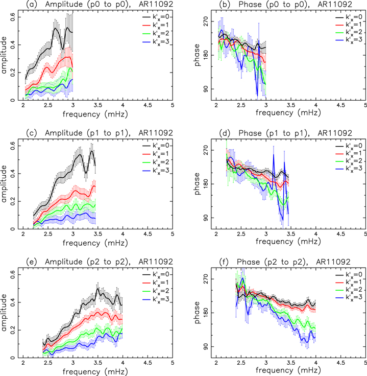
Figure 11. Amplitude and phase of the two-dimensional T-matrix elements  of NOAA 11092 vs. frequency for the scattering from n = 0, 1, 2 to
  , 1, 2, respectively, for various
  , which is in units of Δk = 0.035 rad Mm−1. The error bar of amplitude is estimated based on the amplitude in the noise domain. The error bar of phase is estimated as the arcsine of the ratio of amplitude error to measured amplitude. The data used to create this figure are available.
Download figure:
Standard image High-resolution image
Figure 12. Amplitude and phase of the two-dimensional T-matrix elements  of NOAA 11092 vs. frequency for the scattering from n = 3 to
  , for various
  . The data used to create this figure are available.
Download figure:
Standard image High-resolution image
Figure 13. Amplitude and phase of the two-dimensional T-matrix elements  of NOAA 11092 vs. frequency for the scattering from n = 4 to
  , for various
  , which is in units of
  . The data used to create this figure are available.
Download figure:
Standard image High-resolution image
Figure 14. Amplitude and phase of the two-dimensional T-matrix elements  of NOAA 11092 vs. frequency for the scattering from n = 5 to
  , for various
  , which is in units of
  . The data used to create this figure are available.
Download figure:
Standard image High-resolution image
Figure 15. Amplitude and phase of the two-dimensional T-matrix elements  of NOAA 11084 vs. frequency for the scattering from n = 4 to
  , for various
  , which is in units of
  . The data used to create this figure are available.
Download figure:
Standard image High-resolution imageThe penumbra radii of NOAAs 11084 and 11092 are about 15 and 20 pixels, respectively. The comparison of Figures 13 and 15 shows that the amplitude of NOAA 11092 is larger than that of NOAA 11084, and the amplitude ratio is approximately equal to the square of sunspot radius ratio. For the phase, the values of two sunspots are rather close. This indicates that the amplitude correlates with the sunspot size, while the phase is insensitive to the sunspot size.
The T-matrix element can be obtained from these measured two-dimensional T-matrix element with Equation (9). Since the radial wavefunction  depends only on n and k, the conversion factor is
  , where the equality is based on the dispersion relation and
  . The conversion factor is a real number. Thus the phase of the T-matrix element is equal to the phase of the two-dimensional T-matrix element. For the case of n' = n, the conversion factor is unity for any
  . For the case of
  , one needs to compute the radial eigenfunctions of incident mode and scattered mode at the surface from a standard solar model to obtain the conversion factor. The S-matrix is the sum of the unity matrix and the T-matrix.
One cannot make a direct comparison of the amplitude and phase of T-matrix elements measured here with the results of other methods, such as Hankel analysis (Braun 1995), time–distance analysis (Chou et al. 2009a, 2009b, 2009c), and phenomenological-model analysis (Yang et al. 2012), because the definitions of measured quantities in different methods are different. It is also difficult to find a clear and useful relation between the measured quantities of different methods for comparison.
7. SUMMARY AND DISCUSSION ON MEASUREMENTS
In our analysis, the sunspot is assumed to be time independent, so there is no mode mixing between different frequencies. If the sunspot is time-dependent with a frequency Ω, a mode would mix with other modes with a frequency shift of Ω after interacting with the sunspot (Schiff 1971). Since our two sunspots change little in the observing period (about 7 days), the characteristic timescale for the sunspots is longer than 10 days; the corresponding frequency  mHz. The frequency bin in our analysis is 0.0269 mHz, much greater than Ω. Therefore the assumption of time independence for the sunspots is justified.
The S-matrix (or T-matrix) elements provide the most complete observational or experimental information on the interaction responsible for the scattering and on the properties of the scatterer. In this study, we use the scattered wavefunctions measured with cross correlation and deconvolution to compute the various T-matrix elements. These T-matrix elements provide rich information on the interaction of the acoustic waves with the sunspots and the properties of the sunspots. The properties of these measured T-matrix elements and their implication for the sunspots and the interaction will be the subject of a follow-up paper to avoid making this paper too long. Here we discuss only one implication from Figures 11–15.
All amplitudes of two-dimensional T-matrix elements in Figures 11–15 have a general trend: They increase with frequency for each n and  . Since the horizontal phase speed anti-correlates with frequency for each n, the measured amplitude decreases with the horizontal phase speed for each n. This property provides information on the interaction region, which is responsible for generating the amplitude of the T-matrix element. It suggests that the interaction strength decreases with depth from a depth of about 1 Mm, which corresponds to the the lower turning point of the shallowest mode cavity in our measurements, or a horizontal phase speed of
  mHz. This is explained as follows. The upper turning point of mode cavity changes little with horizontal phase speed, while the depth of its lower turning point increases significantly with horizontal phase speed; that is, a mode samples more and more depth range as its horizontal phase speed increases. If the interaction strength decreases with depth, the influence of the interaction on the mode would decrease as the mode cavity size increases. Therefore, the amplitude of the T-matrix element decreases with the horizontal phase speed. The detailed depth distribution of the interaction strength requires the inversion of measured amplitude. In Figures 11–15, the dependence of the phase on frequency or horizontal phase speed is very different from that of the amplitude and has more complicated features. It suggests that the depth distribution of the interaction region responsible for the phase is different from that responsible for the amplitude. The discussion on this issue is left for a follow-up paper.
In this study, we compute the T-matrix elements with the incident modes of kx = 0 only. Since our measured scattered wavefunctions are for an axisymmetric sunspot, using the incident waves of  would not yield additional information. In fact, for the given
  , the T-matrix elements with an incident mode of
  can be obtained from those with the incident mode of kx = 0 by a rotation transformation, for the case of an axisymmetric scatterer.
Since the data used in our analysis are a time series of 825 frames (about 10.5 hr), and each frame is 250 × 250 pixels (178 × 178 Mm), the resolutions in the frequency and wavenumber domains are 0.0269 mHz and 0.035 rad Mm−1, respectively. Each incident "mode" or scattered "mode" discussed in this study is not really a single mode; instead, it is some kind of average over several adjacent modes within a bin. Each T-matrix element represents the transition between two such averaged modes. Since the wavefunctions used in this study are measured with cross correlation, their phase is relative to the phase of the reference line (initial location of the incident wave), and no random phase is involved as the observed Doppler data (Zhao et al. 2011a). The phase and amplitude of adjacent modes are expected to vary smoothly. Thus the averaged mode should represent the properties of the modes within the bin.
In this study, the T-matrix elements are calculated using the measured scattered wavefunctions through the Fourier transform, as in Equations (11) and (12). It is worth mentioning that the Fourier components in Equations (11) and (12) can also be directly computed from the observed Doppler signals, instead of using the measured scattered wavefunctions. The scattered wavefunction is computed with cross correlation and deconvolution, as in Equation (2) in Zhao & Chou (2013). Thus the temporal Fourier component of the scattered wavefunction from n to n' can be computed with
where  is the temporal Fourier component of the line-averaged observed Doppler signal of n at the reference line
  , and
, and  is the temporal Fourier component of the observed Doppler signal of n' at the point (x, y). Since the spatial dependence of
  is from
  , the Fourier component in Equation (12) can be directly computed from the spatial Fourier transform of
  , which is the temporal Fourier component of the observed Doppler signal. A question arises: Why do we go through the extra step in this study to calculate the T-matrix elements using the measured scattered wavefunctions instead of directly using the observed Doppler signals? The reason is that the measured scattered wavefunction has information on the propagation of the scattered wave packet in spacetime. The scattered wave packet occupies only a limited domain in spacetime. It is easy to identify the signal domain and mask the noise domain before the Fourier transform, as discussed in Sections 5.2 and 5.4. The masking of the noise domain significantly reduces the noise in the computed Fourier components to allow for the determination of the amplitude and phase of the T-matrix elements.
8. DISCUSSION ON INTERPRETATION
The interpretation of measured T-matrix elements will be one of the main topics in a follow-up paper. Here we give only a brief discussion on the connection between the measured T-matrix elements and the interaction of the wave with a sunspot. First we formulate equations for the interaction between the acoustic waves and a sunspot, which is described by a source function. Then the T-matrix element is expressed in terms of an integral of the source function and the quiet-Sun Green's function. The source function, which relates to the subsurface properties of the sunspot, can be inferred from the measured T-matrix elements.
For the quiet Sun, the spatial part of the wavefunction for mode α,  , is the solution of the time-independent wave equation

where  is the time-independent wave operator of the quiet Sun, which involves vectors (Unno et al. 1989). The incident wave is one of the solutions of Equation (14)—for example,
  . In the presence of the sunspot, the operator
  is modified to
  , where the perturbation of wave operator
  describes the interaction between the wave and the sunspot. After interacting with a time-independent sunspot, the frequency remains unchanged and the incident wave
  is converted into
  , which satisfies
Equation (15) can also be expressed as an inhomogeneous equation for the scattered wavefunction 

where  is called the source function which generates the scattered wave
  . For the first-order Born approximation,
  in the expression for the source function is replaced by the incident wave
  .
.
Equation (16) can be solved with the Green's function of the quiet Sun. Since the operator  involves vectors, the solution
  and the source
  have, in general, different directions. Thus the Green's function is a second-rank tensor in three-dimensional space (Jackson 1999). In this study, we use the Greek alphabet to label the modes and the Latin alphabet to denote the spatial directions. The solution
  in direction i can be expressed as
where  is the source function in direction j, and the second-rank tensor
  is the Green's function satisfying

where  is the Kronecker delta, and
  the Dirac δ-function.
With Equation (17), the T-matrix element  can be expressed in terms of the Green's function as
The eigenfunction  and the Green's function
  of the quiet Sun can be solved numerically with a solar model. With the measured
  , Equation (19) can be used to infer the source function
  . For the forward study, given a modeled
  , the T-matrix elements can be computed to compare with the measured values. One can also apply inversion on Equation (19) to estimate the source function
  . From
  , one can infer
  from the known
  .
.
The ultimate goal is to determine the subsurface properties of the sunspot, which include the magnetic field, the thermal perturbation, and the flow in the sunspot region. These properties are the perturbations to the quiet-Sun structure. They would appear in the basic equations, including the mass-conservation equation, the momentum equation, and the energy equation, and in turn would appear in the perturbation of wave operator  . Thus one needs a theory to connect these properties with
  in order to learn these properties from the inferred
  .
.
The SDO/HMI data are provided by the HMI team at Stanford University. M.H.Y. and D.Y.C. are supported by the MOST of ROC under grant NOST-105-21120-M-007-001-MY3.
APPENDIX A: AMPLITUDE AND PHASE DETERMINATION FOR A MODE NOT AT GRID POINTS
In this appendix we discuss the determination of the phase and amplitude of a single-mode signal whose wavenumber is not exactly equal to one of the Fourier wavenumbers. The method is demonstrated with an example of a one-dimensional single-mode discrete signal of N points,

where a is the amplitude and  is the phase; q and p0 label the position and the wavenumber, respectively; and q is an integer, but p0 may not be an integer. We discuss how the amplitude a and phase
  can be determined from the Fourier transform. The discrete Fourier transform of fq is
Here the sign of the Fourier transform is consistent with that in Equations (11) and (12). If p0 is an integer (at a grid point),  . The amplitude and phase of fq are simply the amplitude and phase of the Fourier component
  .
.
If p0 is a non-integer (not at a grid point), Fp in Equation (21) becomes
The Fourier component Fp is nonzero everywhere in the domain of p, but its amplitude peaks at the integer nearest p0. For example, Figure 16(a) shows  vs. p for the case of a = 1,
  , p0 = 11.4, and N = 250 based on Equation (22). The vertical red line marks
  . Note that the data analysis in Section 5.4 also has N = 250.

Figure 16. (a) Amplitude of the Fourier component Fp vs. wavenumber p for a simulation signal fq expressed in Equation (20); (b) phase of Fp vs. p. The non-integer wavenumber p0 = 11.4 is marked by the vertical red line. The black line is the linear interpolation between the phases at p = 11 and 12. The blue cross marks the intersection of the black line and the red line. Its vertical coordinate equals the phase of fq,  .
.
Download figure:
Standard image High-resolution image
The summation of power in the Fourier domain is
This is consistent with Parseval's theorem. Therefore the amplitude of fq is equal to the square root of the summation of power over the Fourier domain.
The phase of Fp is the argument of Fp (between  and π), denoted as
  . Assume p0 is between two integers
  and
and  (i.e.,
  ). From Equation (22), the phases of Fp at
  and
and  are
are


The phase difference between  and
and  is
is  , if
, if  . For our case, N = 250, the approximation creates an error of 4 × 10⁻³. For
  ,
,  , and
, and  for
for  . That is,
  is approximately constant on either side of p0, and the value drops approximately π across p0.
From Equations (24) and (25),  is the linear interpolation between
  and
and  at p0. Figure 16(b) shows the phase of Fp vs. p for the case of a = 1,
  , and p0 = 11.4, based on Equation (22). The vertical red line marks
  . The blue cross sign marks the intersection of the black line and the red line; that is, it is exactly the interpolation of phase at p0. Its value is equal to the phase of fq,
  .
.
In summary, for a non-integer wavenumber p0, the signal in the Fourier domain spreads around p0, and there is a 180◦ phase drop from the grid point smaller than p0 to the grid point greater than p0. The phase of fq (the phase of Fp at p0) can be computed with the linear interpolation between the phases of Fp at two grid points nearest p0. The amplitude of fq is the square root of the summation of  over p. In practice, we need to sum
  over only a small range around p0, because
  decreases rapidly away from p0.