


ABSTRACT
In this paper we describe the synthetic solar spectral irradiance (SSI) calculated from 2010 to 2015 using data from the Atmospheric Imaging Assembly (AIA) instrument, on board the Solar Dynamics Observatory spacecraft. We used the algorithms for solar disk image decomposition (SDID) and the spectral irradiance synthesis algorithm (SISA) that we had developed over several years. The SDID algorithm decomposes the images of the solar disk into areas occupied by nine types of chromospheric and 5 types of coronal physical structures. With this decomposition and a set of pre-computed angle-dependent spectra for each of the features, the SISA algorithm is used to calculate the SSI. We discuss the application of the basic SDID/SISA algorithm to a subset of the AIA images and the observed variation occurring in the 2010–2015 period of the relative areas of the solar disk covered by the various solar surface features. Our results consist of the SSI and total solar irradiance variations over the 2010–2015 period. The SSI results include soft X-ray, ultraviolet, visible, infrared, and far-infrared observations and can be used for studies of the solar radiative forcing of the Earth's atmosphere. These SSI estimates were used to drive a thermosphere–ionosphere physical simulation model. Predictions of neutral mass density at low Earth orbit altitudes in the thermosphere and peak plasma densities at mid-latitudes are in reasonable agreement with the observations. The correlation between the simulation results and the observations was consistently better when fluxes computed by SDID/SISA procedures were used.
Export citation and abstract BibTeX RIS
1. INTRODUCTION
The Earth's state and dynamics are determined by its response to solar illumination. The surface temperature is essentially determined by the absorption of solar radiation power, which occurs mostly in the visible and infrared but has a significant contribution from the near-UV. The spectral distribution of this radiation matters because the surface composition absorbs and reflects back radiation in different degrees depending on the radiation wavelength. This is made evident by the various colors of the ocean and the types of land seen when the Earth's surface is observed from space. Also, the Earth's atmosphere is sensitive to the radiation wavelength because its components have transparency and absorption that are wavelength sensitive. Therefore, an essential quantity for understanding and modeling the Earth's state and dynamics is the solar spectral irradiance (SSI) that couples the Earth's state with the electromagnetic radiation produced in the atmosphere of the Sun. SSI is known to vary over a solar sunspot cycle of 11 years and also in other timescales. In this paper, we study SSI variation with time over about half of the most recent solar cycle, SC24, using our method by which observations of the solar disk or the entire solar surface are employed to model and physically understand SSI. Also, by integration over all wavelengths, we study the total solar irradiance (TSI), which is the total electromagnetic radiation power incident on Earth. We compare results obtained by our synthesis method with existing observations of the UV SSI in this period. This paper first describes briefly the observations and solar disk features considered and specific issues related to the input data used by the SDID algorithms in the present application. Second, the paper describes the behavior found in relative areas of the disk occupied by the features during the five years covered by the present study. Third, we show the application of the feature masks to derive the SSI over the entire wavelength range of 0.05 nm to 600 μm. Finally, we address the application of our results, with emphasis on the UV, to the modeling of the Earth's middle and upper atmosphere.
2. APPLICATION OF THE SDID AND SPECTRAL IRRADIANCE SYNTHESIS ALGORITHM (SISA) METHODS
The Solar Dynamics Observatory (SDO) satellite was launched in 2010 February and started collecting images from its Atmospheric Imaging Assembly (AIA) instrument in 2010 August. The present work uses images from this instrument covering the 2010–2015 period. These images are processed by solar disk image decomposition (SDID) algorithms to construct masks showing the areas of the various features found in the solar disk. The basic SDID method is described elsewhere (Fontenla & Harder 2005) and has been used from its inception in 2005 for studying Ca ii K images from the Mauna Loa Solar Observatory, later extended to similar images from other observatories and various instruments as well. The method was created by S. Davis and J. Fontenla (unpublished); there is also a different method previously studied by P. Fox, which we neglect here. In the present paper, we explain important details of the application of SDID to the AIA images. The images used in the present study are mostly from level 1 processing by the Joint Science Operations Center. SDID procedures do not rely on absolute intensity calibration; rather, the calibration of each image is determined from the data in a semi-empirical way to determine a uniform reference level. This image self-calibration is in relative units, and its purpose is only to produce homogeneous quality feature discrimination over an extended period of time while imposing the minimum possible biasing in the results. From the daily (or more frequent) feature masks produced by SDID, the SISA is used for the computation of SSI by combining the angle-dependent spectra for each feature. This algorithm for constructing the SSI remains basically the same as in Fontenla et al. (1999), but the physical models of the features and the feature spectra have largely improved since then throughout the extensive analyses of new and old observations by Fontenla et al. (2014, and 2015), new atomic data, and a much more complete full-non-LTE method that supersedes the approximate one carried out in 1999. The emitted spectra of the current physical models were calculated using Solar Radiation Physical Modeling version 2 (SRPMv2), as shown in Fontenla et al. (2011, 2014, and earlier). They are slightly modified, at some wavelengths, here in consideration of the very detailed near- and far-UV observations and atomic data described by Fontenla et al. (2015). During the time period we consider, solar cycle 24 (SC24) activity rose from a minimum in 2009, slightly preceding the present study, to the solar maximum and has been slowly decreasing, but at the time of this paper's submission, the Sun is still in a significantly active state. Therefore, our study does not cover the entire SC24 because the data used do not extend exactly to the previous minimum or reach the end of the cycle (which can only be fully defined after the next complete minimum occurs).
Unlike other methods, e.g., those of Henney et al. (2012 and 2015), SDID and SISA do not use magnetograms and consequently do not rely on a relationship between the magnetic field and the emitted intensity. Our methods are simply based on a classification of the observed emitted intensities in images of the solar disk at several key wavelengths. Depending on the wavelength and the position on the solar disk, each of the intensity ranges indicates the presence of a certain feature for which a physical model, derived from many detailed observations, is available.
The vertical extension of photospheric and chromospheric features is relatively small compared to the spatial resolution of available instruments, in the present cases in AIA, so that these features can be approximated by a planar one-dimensional model whose properties only depend on the height above the photosphere. Although a fine-scale horizontal structure exists at scales smaller than the AIA observation resolution of ∼1 arcsec (e.g., as shown by Hinode; see Suematsu et al. 2008), our models assume a one-dimensional atmosphere that describes independent vertical columns of material that is able to successfully reproduce the observed spectra at most wavelengths. This assumption was discussed in our previous papers. Because there is no absolute height reference in our models of each feature, it is expected that structures very close to the limb that extend at larger heights can obscure or completely block structures at lower height. This effect is clearly observed in sunspot umbrae because of the well-known Wilson depression but is not as clear in other solar features and is not critical to the present application.
The currently considered set of features is defined by Fontenla et al. (2014) and is listed in Tables 1 and 2, for the photospheric/chromospheric and coronal features, respectively. These features were listed in papers by Fontenla et al. (2011, 2014, 2015, and references therein), where atmospheric models for each feature were presented and the radiance spectra for each feature were shown. Note that the radiance spectra of all features are dependent on the observing angle with respect to the solar radial direction. This effect is known as center-to-limb variation because the angle is zero when observing the disk center but is near 90° when observing the solar limb. In all cases, except in coronal holes, we discriminate the feature in each pixel by using intensity thresholds applied to the intensity images obtained by AIA. The SDID algorithm applies a fixed set of center-to-limb-dependent relative thresholds to establish which category each pixel belongs to, and produces a mask file. Combining the masks obtained from the images at various wavelengths produces a pair of masks per day, one for the chromospheric features and one for the coronal features.
Table 1. Current Models for the Solar Disk Chromospheric Features
| Feature | Description | Model Index |
|---|---|---|
| A | Dark quiet-Sun inter-network | 1500 |
| B | Quiet-Sun inter-network | 1501 |
| D | Quiet-Sun network lane | 1502 |
| F | Enhanced network | 1503 |
| H | Plage (that is not a facula) | 1504 |
| P | Facula (i.e., very bright plage) | 1505 |
| Q | Hot Facula | 1308 |
Download table as: ASCIITypeset image
Table 2. Current Models for the Solar Disk Coronal Features
| Feature | Description | Model Index |
|---|---|---|
| CA | Coronal Hole | 1310 |
| CB | Quiet-Sun inter-network | 1311 |
| CD | Quiet-Sun network lane | 1312 |
| CF | Enhanced network | 1313 |
| CH | Plage (that is not a facula) | 1314 |
| CP | Facula (i.e., very bright plage) | 1315 |
| CQ | Hot Facula | 1318 |
Download table as: ASCIITypeset image
The association of the measured intensity of the pixels in the observed image as belonging to one of the features, in Tables 1 or 2, depends on the channel(s) used. To identify each feature using the AIA images, we use the channel that provided better discrimination for that particular feature. The image types are identified by the filters' nominal wavelengths, but we warn the reader about the very broad wavelength ranges of these images, which are addressed in a later section. For example, images in the 450 nm channel are used to identify areas of the solar disk corresponding to sunspots. Images from the 160 nm channel are used to discriminate quiet-Sun chromospheric network features as well as the active network, which for our purposes is indistinguishable from the very bright quiet-Sun network. Images from the 19.3 nm channel are used for chromospheric active region plage and facula features in the chromospheric masks. Images from the 9.4 nm channel are used for coronal masks identifying the coronal plage, facula, and very bright facula. A different procedure is described below for coronal holes. Quiet-Sun coronal features are not identified in the coronal images because they are not well distinguishable. The interpretation of the coronal images' correspondence to features is more complicated than that of the chromospheric or photospheric ones because of the small optical thickness of the coronal radiation. Many very bright pixels in the images correspond to very-low-altitude coronal temperature material and belong either to the upper part of the legs of coronal loops or to very-low-altitude unresolved loops. However, there are also fainter contributions from larger-altitude loops that span many pixels in the images and whose brightness identification is also unclear because the top of very bright loops may have an intensity level similar to that of a nearby footpoint of another very different loop. An additional issue is that the temporal evolution of individual loop coronal structures differs from loop to loop: some evolve significantly over timescales of minutes, while others apparently evolve in hours. However, this can be a resolution-dependent issue because slowly varying loops could be composed of smaller unresolved, fast-evolving loops. Trying to follow the behavior of each individual loop in detail is neither practical nor useful for SSI modeling, because outside of flares the contribution of an individual loop is not important. Instead, the statistical behavior of the groups of loops is what matters. For this reason our coronal feature models remain one-dimensional models of relatively compact areas corresponding to ∼2 by 2 arcsec pixel in extreme-UV (EUV) observations and describe only a statistical behavior and not individual loops. Faint extended loops are not identified in the current SDID masks. To properly describe the extended groups of coronal loops, a three-dimensional group of loops model is needed together with the means to infer the group's three-dimensional structure from images. This structure is very hard to infer from coronal observations but could be assessed by realistic magnetic field extrapolations, which are proven to be consistent with observations. The inclusion of faint extended loops on the disk or above the limb would be a further improvement that is not critical at present.
3. IMAGES AND MASKS OF THE SOLAR DISK
3.1. Self-calibration of AIA Images Used
An issue for the SDID method is the absolute intensity calibration of the AIA images used because a shift in the reference intensity could affect the feature identification, especially in the 160 nm channel. For this reason, we have developed an image self-calibration method whose purpose is to establish a reference intensity level based on quiet-Sun pixels, and we use this method for removing instrument degradation effects.
Our method relies on determining, for each image, the intensity levels relative to a reference intensity obtained from the image itself. The procedures we describe here allow us to determine the reference intensity value as a function of the observation angle, and we have applied them to each of the 1428 chromospheric and 1658 coronal images.
Figure 1 shows the AIA image of a circular area with a 4 arcmin radius at the disk center for the first good AIA image in our set, taken on the same day of every year starting on 2010 August 20, and for the same day and area for 2011, 2012, and 2013. The data shown in the left panels include no active regions, while those in the right panels encompass strong active regions, easily identifiable due to the far larger intensities in the 19.3 and 9.4 nm filters. Their intensities are also larger in the 160 nm filter, but the contrast is not as large. We select these few images and areas to illustrate the self-calibration procedure we use to determine the intensity levels in each image relative to a reference intensity level obtained from the image itself. The procedures described here to determine the reference intensity value as a function of the observation angle are applied to each of the 1428 chromospheric and 1658 coronal images.
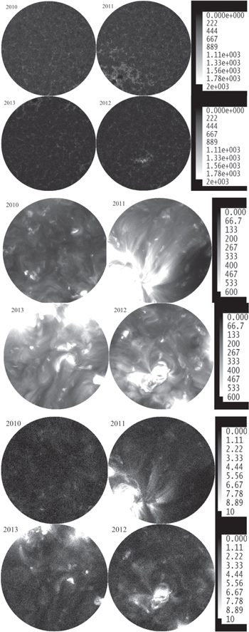
Figure 1. The center of the solar disk in three AIA images on the same day every year starting on 2010 August 20. Top, 160 nm; middle, 19.3 nm; and bottom, 9.4 nm. The circles shown correspond to a 4 arcmin radius at the center of the disk.
Download figure:
Standard image High-resolution imageFigure 2 shows the intensity histograms for the areas of the disk shown in Figure 1. Again, we split the dates into two sets of panels. In the left panels, very little of these areas was affected by active regions. In the right-panel data, a significant part of the selected areas was occupied by active regions. This is also shown by the larger number of pixels in the far tails of the distributions. The intensity histograms in Figure 2 correspond to absolute counts from the images, and their shapes are far from a Gaussian distribution: because of the tail of the intensity distribution and its variation in time, a simple average is not a good definition for a reference intensity level. By contrast, the median has the advantage of neutralizing the effects of the very large intensity pixels belonging to active regions and provides a much better reference, albeit still affected to some extent by changes in the tail of the intensity distribution. For this reason, we carried out the analysis that follows.

Figure 2. Intensity histograms of circular areas at the center of the AIA images. The left panels correspond to mostly quiet areas, and the right panels to areas that had significant activity. For the 160 nm case, we chose a different scale in the right-side panel to show the details of the low intensity range.
Download figure:
Standard image High-resolution imageThe 160 nm Channel data generally show a shape with some resemblance to the log-normal shown by Fontenla et al. (2007) for a much narrower spectral band at 160 nm and based on the Solar and Heliospheric Observatory (SOHO)/SUMER instrument. Also, Fontenla et al. (2009a) showed a similar log-normal intensity distribution in the C i continuum, and Warren et al. (1998) found it earlier in chromospheric lines. We believe this distribution results from the chromospheric heating of the quiet-Sun, but the parameters of the distribution shape depend also on the particular line or continuum observed and not only on the heating mechanism. As expected, there are some clear differences from previous data because of the particular spectral region included in the AIA images. The spectral response of the images is discussed in the next subsection. Many details could be pointed out in Figure 2, but for brevity we only stress that (a) comparison of the left and right panels clearly shows that the high-intensity extension of the distribution largely increases with solar activity and the slope of this extension decreases and (b) for the histograms of the AIA 160 nm channel, the peak of the distribution shifts toward lower values as time elapses, but this shift is apparently independent of the activity level.
We consider the apparent shift of the peak of the distributions in the 160 nm case and, to a lesser extent, in the 19.3 nm case to be due to AIA instrument degradation and not to a solar effect. For the 9.4 nm channel a low intensity peak is not clearly seen, but only a tail of a decreasing number of pixels with increasing intensity is present. A simple interpretation, justified by the images, is that in the 160 and 19.3 nm intensity histograms the interval around the peak of the distribution corresponds to the center of the network cells. At around the 400 and 4 intensity counts, for 160 and 19.3 nm, respectively, a brighter distribution of pixels occurs in the network lanes. The intensity distribution of these brighter pixels merges with the high-intensity tails from active regions. The tails of the distributions have a very variable level, a flatter slope, and a high-intensity cutoff. In order to eliminate instrument degradation issues and produce a self-consistent identification of solar features free from instrument biases, we use the histogram shapes to replace the raw intensities addressed above with relative intensities with respect to a reference value defined by the peak of the raw intensity distribution. In the past we used the histogram's median as the reference intensity that corresponds to feature B; now we instead use the peak of the distribution as the reference level because we find this more reliable. Figure 3 shows the relative intensity histograms that produce a much more consistent description than the raw intensity histograms. The histograms in Figure 3 also indicate that, in the 160 nm images, the change in slope at around 3 in the relative intensity distribution had a smaller area in 2010 than in later years and is sensitive to the presence of solar activity even outside typical active region pixels. A somewhat similar effect is noticed at 19.3 nm, but in these data the change of the slope of the distribution is not as clear. The 9.4 nm images do not show a bump at any intensity level, and it is unclear whether the images show any network pixels detectable above the noise.
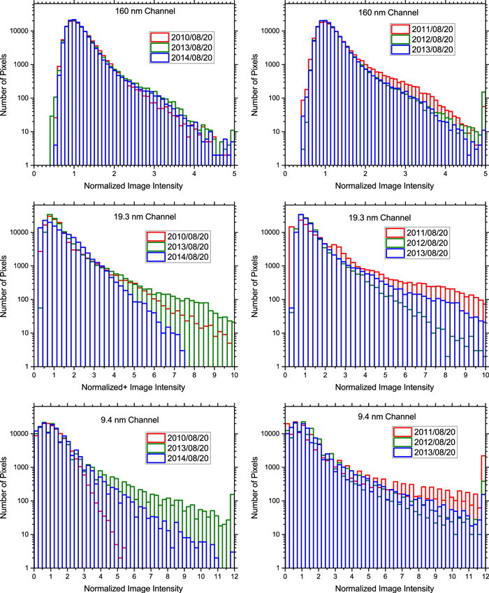
Figure 3. Relative intensity histograms of the circular areas in the center of the AIA images. The left-panel data correspond to mostly quiet areas, and the right-panel areas had significant activity.
Download figure:
Standard image High-resolution imageAn important point to consider is that the general shape of the relative intensity distributions near the disk center is fairly well defined, at least for similar activity levels, but this shape and the relative intensity at the peak of the distribution are dependent on center-to-limb effects. The SRPMv2 calculations using the AIA spectral responses show that the 160 nm AIA data are expected to show limb darkening (in spite of the monochromatic 160 nm continuum radiation having a neutral center-to-limb behavior), and other channels are expected to show limb brightening, consistent with observations. For this reason, in SDID, the solar disk is subdivided in a set of annuli (usually 10 at equal intervals of Δμ = 0.1, where μ is the cosine of the observing angle with respect to the solar radial direction; see Fontenla et al. 1999; Appendix B). The histogram peak values in each of these intervals are independently determined. In this way and by using a cubic spline interpolation, SDID defines an intensity normalization function that varies smoothly between the values found at any μ values in each observation. This procedure works very well except very close to the limb, where strange effects arise from small errors in the determination of the image center and radius, from aliasing, and from projection effects due to the vertical extent of solar atmosphere features. In the present application of SDID, we disregard the classification of pixels for μ < 0.1 (i.e., R ∼ 0.995 Rs) and instead label them as feature B. Several tests have shown that this assumption does not substantially affect the results, although it produces a very slight bias toward feature B.
3.2. Spectral Characteristics of the Images
The spectral transmission of the AIA filters is known, although it does not always cover the entire wavelength range that would be desirable; Figure 4 shows the best data we have about these. These transmissions are relatively broad and encompass substantially more than their nominal spectral lines. In some cases the nominal line is the major contribution in the quiet-Sun, but in pixels where strong activity is present, other lines may dominate. SDID does not rely on the nominal wavelengths of the AIA channels but instead convolves the spectral transmission of each filter and the SRPMv2-computed spectra for each solar feature and each angle to calculate the expected AIA contrast at each of the ten selected disk positions. These contrasts are represented by a two-dimensional table that describes the thresholds for identification of the various features at each disk position and for a given filter. These tables are realistic because they rely on the entire coronal and chromospheric spectra and complete line and continuum dependencies on the atmospheric model without any further assumption. However, SDID also compares these tables with the contrast observed in the images and finds general agreement. In some cases minor corrections are applied to the table of contrasts to better discriminate the solar features, and the corrections can be due to inaccurate or incomplete knowledge of filter spectral transmissions. The general agreement we find is not surprising because the physical models of the features were derived by SRPMv2 to match the observed radiance spectra.

Figure 4. Filter transmission for the used AIA filters and SRPMv2 spectra for two features of the chromosphere and of the corona at the disk center and at 0.1 nm resolution. The red and green curves correspond to the computed photon flux at 1 au (scaled by 10−13) for models 1501 and 1505, and 1511 and 1515 (corresponding to features B and P, and CB and CP, listed in Tables 1 and 2). In the right panel the coronal component is very small and was not plotted.
Download figure:
Standard image High-resolution imageFigure 4 shows the filter profiles and the spectra for a few features, at the disk center, that were computed by SRPMv2. Filters 9.4, 13.3, and 19.3 have a spike at their nominal wavelengths but also extend to wavelengths far from their nominal value. For filters 9.4 and 13.3 nm the tail reaches many lines of large flux that extend at wavelengths longer than 15 nm. In the case of 19.3 the long wavelength tail is somewhat sensitive to the He ii 304 line which forms in the low transition region. Also, this channel has a secondary bandpass at very short wavelengths. Furthermore, while in the quiet Sun a certain line may dominate the bandpass, in active regions other lines may dominate or at least contribute to the images. The 160 nm filter is very broad and includes the Si i and Fe i continua in addition to a number of spectral lines that include the strong C iv and Si iv and the C i, Al ii, and He ii ∼164 nm lines. These inclusions are not a critical issue for SDID because most of these emissions are controlled by the illumination from the upper chromosphere. Some lines are directly formed in the upper chromosphere, the continua form in the temperature minimum region but are determined by the illumination from above, and the other lines form in the lower transition region at or below 105 K, and in all features their intensities are very closely related to the upper chromosphere. Therefore, regardless of the details of the spectrum included in the wide bandpass, the images from the 160 nm channel are good indicators of the heating of the upper chromosphere. The chromospheric character of the AIA 160 nm images is made obvious by the appearance of the images; however, the SDID bases in our detailed spectrum study show to which degree the transition region or coronal material can affect identification. Comparing the contrast of the surface features in some selected images with those predicted by the two-dimensional table mentioned above shows general agreement. In the 160 nm AIA images, the calculated and observed contrast values corresponding to the network and active regions are large and very good for discriminating the network cells and enhanced network—features A, B, D, and F. However, the contrasts corresponding to features H, P, and Q are very similar and indicate that the identification of the active region components would be less precise if these images were used. Because of this, the AIA 19.3 nm channel images are used for identifying the chromospheric plage areas in the images. The active region features are very bright and are easily discriminated in these images, but occasionally they may become contaminated by the transient apparition of post-flare loops. The present work did not carry out special processing to eliminate these transient events, and therefore, the SDID processing might overestimate the plage areas in these cases.
Figure 4 also shows the transmissions of the 13.3 and 33.5 nm AIA channels that are used to discriminate the coronal-hole pixels. This determination is done in a different way from that of the other coronal features. SDID identifies coronal holes by comparing the 33.5 and 13.3 nm channels' intensities. This is a good coronal temperature diagnostic because the former band is mostly sensitive to the plasma at temperatures below ∼1.2 MK and instead the 33.5 nm band contains several lines produced by plasma at temperatures above that value. The net result is that differencing the weighted intensities in the two bands and normalizing the difference by the weighted sum yields a value representative of the plasma temperature that indicates the predominant temperature of the coronal plasma at each pixel. Of course, it cannot be claimed that a single temperature value is present in a pixel, and in fact our coronal models have plasma at many temperatures from a maximum value down to 0.2 MK in the transition region. Indeed, our diagnostic points toward the maximum temperature reached for a significant extension of the corona. A formal justification of the procedure we use is not possible at present because of the multithermal nature of the coronal plasma, in both the vertical and the horizontal dimensions. The parameters necessary to implement this procedure have been determined in a semi-empirical way. Furthermore, we mark as black pixels those where the sum of both channels' intensity is below a specified number. In these pixels, the signals from both channels are so noisy that a clear feature identification cannot be made. The designation of coronal holes in this work is exclusively focused on the SSI, and areas designated here as coronal holes include the polar holes, the equatorial holes, filament channels, and often small areas neighboring strong vertical magnetic fields. From the point of view of the SSI there may not be a need to distinguish between these structures. Figure 5 shows examples of chromospheric and coronal masks constructed by SDID.
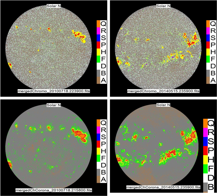
Figure 5. Top: sample chromospheric masks showing (left) a day with only plage visible and no noticeable sunspots and (right) another mask with active regions including numerous sunspots. Bottom: sample coronal masks showing the same days as in the chromospheric masks above but without discriminating between quiet-Sun features CB and CD because they cannot be clearly identified in the SDO/AIA images. Coronal holes (feature CA) are shown as brown areas.
Download figure:
Standard image High-resolution image4. FEATURE RELATIVE AREAS' TIME SERIES
Figure 6 shows the temporal variation of the total relative areas of the features (TRAFs). These TRAFs are the ratios of the accumulated number of pixels for each feature over the solar disk divided by the total number of pixels of the solar disk in each mask. Note that SDID produces much more information than these TRAFs, such as information about the observation angle, which is also useful for computing the SSI, and information about the latitude and longitude of the active regions, which is very useful for studying properties of the solar cycle. The chromospheric and coronal masks of the solar disk were computed for the period of this study, 2010–2015, and are currently produced and posted on the website http://www.galactitech.net/John/SERFS/Images/. The panels in Figure 6 show the TRAFs as a function of time. In 2010 the sunspot TRAF (the sum of the umbra and penumbra) was above zero but very small, ∼3e-4. It rose rapidly around 2011 September to peaks of ∼1.5e-3 and then decreased again in the beginning months of 2012, forming what we call the "first bump" of solar activity. In this first bump the penumbra and umbra TRAF were similar, and little rotational modulation (RM) occurred because these sunspots appeared almost uniformly distributed in longitude, although they were preferentially located at relatively high latitude, in both hemispheres, and were more numerous in the northern hemisphere. Then, a "second bump" in sunspot TRAF occurred for a few months before and up to 2012 September that reached peaks of ∼0.004 but rose and decayed more rapidly; also, it had a larger ratio of the penumbra to the umbra than the previous bump. The images show that this second bump was produced by several active regions with large sunspots that appeared suddenly in the southern hemisphere and had important RM. This RM corresponded to the predominance of a preferred range of longitude in the southern hemisphere's active regions. After these striking early bumps, the solar cycle continued with strong RM (in fact the best defined in the current solar cycle) and other bumps of generally decreasing umbral TRAF, although the activity remained significant with the penumbral TRAF hovering around a value of 0.001. To date, the current cycle, SC24, has not shown very important overall sunspot areas except during the second bump. The chromospheric active region areas also showed the first and second bumps described above, but the second one did not have very large TRAFs, and the marked RM again starts after the second bump. After these two bumps, the TRAF of plages and faculae, features H and P, started increasing until it leveled around 2015 September and then started decreasing. Both show strong RM and in recent times a similar peak TRAF of faculae and plages that reach areas of nearly 0.02 each and show a very asymmetrical distribution over the solar surface into two separate general longitudes. This panel also shows the TRAF of the regular network (feature E) decreasing while the more active features replace it. The feature masks (not shown) indicate that the enhanced network, feature F, in the TRAF plots of Figure 6 sometimes appears in some very isolated areas and at other times is contiguous to active regions. Figure 6 also shows that the TRAF of feature F seems to remain practically constant in time, but the masks indicate that some patches appear at the expense of previously quieter areas, while others disappear by transforming into plages. It is also interesting that sometimes, large patches contiguous to active regions appear where an enhanced network seems to be almost absent. The formation of these patches seems to be random, and we do not understand the context in which they are produced. In any case, SDID masks clearly identify the locations in every case, but a full enhanced network discussion is outside the scope of this paper and requires additional study to be published in a separate paper. Perhaps the most complex variations of TRAFs occurred for the quiet-Sun features. A strange balance appears in the overall variations of features A, B, and D, but it must be kept in mind that not all TRAFs are independent and the sum of all is unity by definition. An interesting decrease in the area of the average cell center, feature B, reached a local minimum in 2011 November and corresponded to the first bump increase in active region features. As with the features above, around 2012 August a more or less regular RM started. In other quiet-Sun features, the RM is not as important, and we attribute that in feature B to increases in the active region features.
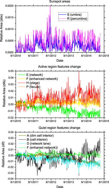
Figure 6. The temporal variation of the areas of the disk covered by the chromospheric features.
Download figure:
Standard image High-resolution imageFigure 7 shows the TRAFs of coronal active region features and of coronal holes. The active region features (CF, CH, CP, and CQ) started increasing before 2011 August and display the same first bump as the chromospheric active region features. However, they did not show the second bump and instead showed a relative minimum that was followed by a large RM, as in the chromospheric features. Afterward, the general level followed a trend similar to that of the chromospheric active regions. A very interesting behavior is shown by the coronal holes (feature CA). These were at a level of ∼0.04 in 2010, but they first suddenly decreased at the beginning of the first bump, then started increasing at the start of the second bump, plummeted again at the end of the second bump, and from then started increasing until they reached the present level of ∼0.18. As with nearly all other features, the coronal-hole TRF displayed a strong RM around 2012 August. While the polar coronal holes were nearly absent in 2010, they are currently present, along with a number of coronal holes in various locations at lower latitudes. The shape of many of these holes suggests they correspond to filament channels.
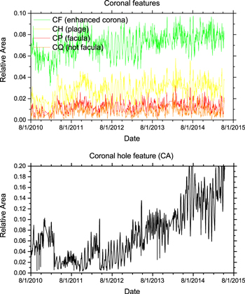
Figure 7. The temporal variation of the areas of the disk covered by quiet-Sun (top) and coronal hole (bottom) features.
Download figure:
Standard image High-resolution imageIn summary, the present SC24 has been rather complicated so far, and perhaps the clearest pattern has been the persistent growth of the TRAF of the coronal hole feature by a factor of ∼5. There can be instrumental effects on this finding. We can only mention the possibility that the AIA 13.3 and 33.5 nm channels are degrading differentially and that this may affect the comparison used to define the coronal-hole mask in SDID. However, another possibility is that there might be a real solar process of building polar coronal holes and near-radial magnetic fields.
5. SSI TEMPORAL VARIATION
Using the complete SDID results, we applied the SISA algorithm to the period 2010–2015 to compute the entire SSI at several spectral resolutions in several bands as well as the TSI. Note that the SISA algorithm does not require the computation of the time dependence of the entire high-resolution spectra for the computation of particular bands or even the TSI. For the present times, some results are posted on the website http://www.galactitech.net/John/SERFS/Images/ under the links shown there.
5.1. Near-UV, Visible, and Infrared Spectral Range
The solar radiation in this spectral range originates essentially in the solar photosphere and lower chromosphere, but some contributions of absorption and emission lines are produced in the upper chromosphere. Upper chromospheric lines are scattered through the spectra but are densely distributed and more important at the shorter wavelengths. The overall solar spectra and their details were shown in our previous papers (e.g., Fontenla et al. 2011, 2014, 2015) and will not be repeated here. Instead, this paper will focus on the time variation of the SSI over SC24.
Figure 8 shows the time evolution of the SSI in the UVC and UVB spectral bands. These bands have significant effects on the Earth's middle atmosphere and on the stratospheric ozone. The UVC SSI band is completely absorbed in the atmosphere, but UVB radiation reaches the stratosphere and a small part even reaches the ground. The overall energy in these bands, especially in the UVC and UVB, is about 30 W m−2, a small but significant part of the TSI. Even if its variability is not very large, it is much larger than that of the TSI and can be significant to some processes in the Earth's troposphere. Biologic photochemical processes are sensitive to UVB radiation but not to longer wavelengths, which would only produce heating. The SSI variation in the present SC24 was not particularly large, but its spectral details are significant in the relationship with the very variable atmospheric absorption, and the combination of both determines the amount of near-UV radiation reaching the ground. The variations shown in Figure 8 indicate some activity already occurring in late 2010 and rapidly increasing in 2011 with a few isolated peaks later. The first bump in solar activity is observed with a width of about six months and a broad maximum around 2011 November and a weak RM. A sudden peak with a few days' duration also occurred within that bump. Larger-amplitude RM occurred around 8/1/2012. The maximum non-flare near-UV SSI was reached around 2014 February; recently, the SSI at these wavelengths started slowly decreasing. This type of computed behavior is qualitatively similar at all wavelengths that are strongly affected by chromospheric lines because it is driven by the same active region and network features shown in Figure 6; however, the quantitative details vary depending on the sensitivity of lines to the presence of each particular feature. In 2011 some long-duration event (X-ray classification M1.3) was randomly captured on October 22; in 2012 a number of X-class flares occurred that were not sampled by our spread data during that year; in 2013 a significant spike corresponds to the flare on June 23 (class M2.9), which again was a long-duration event; and in 2014 the largest spike shown in Figure 8 corresponds to the X4.9 large flare whose decay was captured in our February 24 data. However, the methods we use are generally inadequate for flares because of their non-thermal particles and relatively fast evolution. Figure 9 shows the temporal variations of the SSI at visible and infrared wavelengths. These wavelengths are more affected than the near-UV by the presence of sunspot umbrae and penumbrae, shown in Figure 6, which cause the SSI to decrease. In fact, the darkness of these features in the continuum decreases the SSI, but the chromospheric lines that are bright in the plage and facula over-compensated this decrease in the UV. The effect of the lines still dominates in the UVA but is weaker in the visible bands as lines become sparser and the effects of the continuum become more important than those of the lines. This is also the case in much of the IR, but in certain bands, e.g., the CO bands, the lines can again dominate. However, during SC24, the overall sunspot areas have been relatively smaller than in previous cycles in relation to the other active features (enhanced network, plage, and facula), and the calculations shown here have produced an overall increasing TSI until now, as shown in Figure 10.
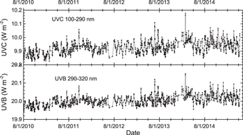
Figure 8. Time series of SSI variations in several near-UV bands.
Download figure:
Standard image High-resolution image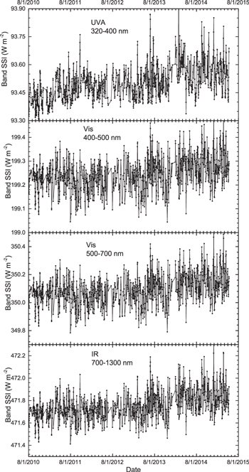
Figure 9. Time series of SSI variations in several visible and infrared bands.
Download figure:
Standard image High-resolution image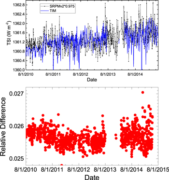
Figure 10. Top, comparison of the total solar irradiance time series observed by the SORCE/TIM instrument and the present synthesis results of combining SRPMv2 and SDID/SISA. The symbols indicate the times of the synthesis results; the TIM data are daily averaged and plotted at noon. Bottom, scattered plot of the TIM data and the result of averaging the available synthesis results on each day. On most days, the synthesis results have a single point; sometimes, an average of two points; and very few times, an average of several points.
Download figure:
Standard image High-resolution imageThe top panel of Figure 10 shows the synthesized TSI compared with the measurements made by the TIM instrument on board the SORCE satellite. Consistent with the temporal behavior in the spectral bands shown before containing most of the SSI variability, the TSI overall increased during SC24. The scaling factor applied to the computed TSI reflects the ∼2.5% overestimate of the calculated TSI from the SRPMv2 physical models (see Fontenla et al. 2015). However, it must be noted that the TIM data shown in Figure 10 correspond to daily averages (labeled at noon), while the computed TSI is calculated using a few images per day taken at random times during the day and is often insufficient for establishing a daily average. For this reason, the TIM daily data is expected to have fewer fluctuations than those computed from snapshot measurements by SDID/SISA, which may include intra-day variations and even flares. Moreover, fluctuations of the synthesized data are also expected from the image quality and limb issues described in Sections 2 and 3; in addition, the data are severely affected by the poor quality of the SDO/AIA images in the 450 nm channel, which we used here for the identification of pixels corresponding to the sunspot umbra and penumbra. This last issue is shown by the scatter of points on the bottom panel of Figure 10 and results in noise on the top panel of Figure 6 and in increased noise in all visible wavelengths shown in Figure 9. We tried to flat-field the 450 nm images as much as possible, but strange image defects exist that vary in time after apparent "events." Consequently, only part of the increased variability in the synthesis is real. However, despite the problems in the 450 nm channel, the artifacts in the TSI are small in relative terms, thereby affecting the rotational variability but having little effect on the observed solar cycle trend, of ∼735 per million (ppm), which is well represented by the synthesis. This is also illustrated by the bottom panel of Figure 10, which shows no important trend in the general level of the scattered points but suggests only that, after an initial "event," the scatter of the points increased with increasing time and reached a maximum of ∼500 ppm, but with outliers beyond that scatter.
Because of the issues described above, we find that the set of SDO/AIA images we used is not very good for reconstruction of the visible and IR rotational variability because of the noise introduced by the poor quality of the 450 nm channel. However, the synthesis performed here gives an adequate representation of the solar cycle trend, and better observations at visible wavelengths could solve the RM issue.
5.2. SSI Spectrum Comparison with EUV and FUV Observations
The SSI variation at EUV wavelengths has important consequences for the Earth's upper atmosphere because despite the overall relatively small energy of SSI, it is completely absorbed in the tenuous layers above the stratosphere. However tenuous, these layers affect low Earth orbit satellite drag and the propagation of radio waves and therefore are relevant to modern human activity. In previous papers (Fontenla et al. 2014 and 2015) we have shown in detail how the SRPMv2 spectrum compares with several isolated UV observations, and for brevity we do not repeat such comparisons in this paper. That work also showed the spectral variation of a typical large-RM case. An important application of the SDID/SISA results is the calculation of far-UV (FUV), EUV, and XUV SSI, each of which is an important driver of the variability of neutral density and ionization of the Earth's upper atmosphere. These variations were initially correlated to the F 10.7 cm flux (e.g., Covington 1969; Mahajan 1967) because it is the longest and most comprehensive absolute measurement of solar activity, even if the radiation at this wavelength is not important for the Earth's atmosphere. The effects of solar variability on the upper atmosphere layers depend on the spectral details of the SSI because different wavelengths produce heating and photochemical effects at different altitudes depending on the Earth's atmospheric absorption and photochemistry cross-sections. Solar activity manifests itself in increased SSI throughout the entire UV spectrum, but there is no single scaling that can be applied to the SSI because radiation at different wavelengths is produced by different physical processes and often in different locations of the solar atmosphere. Neglecting this complexity, Hinteregger (1981) developed a simple "proxy" model for the solar radiation in certain bands, and EUVAC was developed by Richards et al. (1994) using the F 10.7 cm flux as a "proxy" and an empirical linear scaling for certain wavelength bands, or bins. However, the F10.7 index, i.e., the radio flux at a wavelength of 10.7 cm, is produced at and above the layer of the solar atmosphere where the optical depth is unity, which in the quiet-Sun is located around the temperature minimum, but in active regions it is produced by
- 1.free–free emission (bremsstrahlung) with an emissivity that depends mostly on the square of the electron density; and
- 2.cyclotron emission, which depends on the product of the electron density and magnetic field strength.
Instead, the lines that dominate the emission in the EUV and XUV form higher in the solar atmosphere and are sensitive to the electron density and, most importantly, to the temperature of the material in the corona and chromosphere–corona transition region. The same is true for the FUV lines, and indirectly, it is also the case for the FUV continuum. Historically, the EUVAC model has been developed and used for a long time for modeling the upper atmosphere's neutral density because of the lack of a complete and continuous record of UV SSI. However, measurements show that the EUVAC model provides an approximate estimate of the SSI but is inaccurate at least in some cases (e.g., Donnelly et al. 1986). Also, accuracy has become increasingly important for the modeling of neutral density that is used to track objects in the currently very congested low Earth orbit.
Figure 11 shows the comparison of the observed F10.7 index with the Lyα composite (downloaded from the LASP Interactive Solar Irradiance Data Center) and the presently synthesized composite multiplied by a factor 1.3 (the current calculation underestimates the lower transition region lines by about 20%–30% because of the slightly lower pressures mentioned in Fontenla et al. 2015). This underestimation will be corrected in later papers, but for now we account for it by applying a factor 1.2 to the transition region spectra because in previous papers we have shown that the transition-region line emission scales linearly with the pressure. Some spikes in the computed Lyα result from flares; also, the F10.7 and composite data points are daily averages, but the computed data resulted from snapshot images and did capture some flares but missed others. We are not sure of the composite but assume daily average values for it as well.
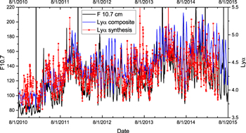
Figure 11. Measured F10.7 in SFU units (black), scaled Lyα composite (blue), and computed (red, multiplied by 1.3) Lyα +−0.5 nm flux in units of 1011 photon s−1 cm−2.
Download figure:
Standard image High-resolution image5.2.1. Empirical Models of the Earth's Upper Atmosphere
Among the empirical models of the upper-atmospheric neutral density, the early models by Jacchia (1971) defined an example of an empirical atmospheric model and found a correlation of satellite drag with F10.7 (Jacchia 1969). The JB2008 by Bowman et al. (2008) considers, as SSI proxies, some operational indices defined by observations from particular space-based instruments, in addition to the F10 index based on the F10.7 cm radio flux. A problem with this approach is the limited instrumental lifetime, because when a new instrument replaces an older one, the continuity and self-consistency of these measurements are lost. Besides, space-based instruments generally suffer degradation that is very hard to accurately correct and results in significant drifts. Moreover, the use of other proxies and statistical correlations, although better than the F10.7 cm proxy alone, does not physically explain the atmospheric processes involved, and while it could work for past observations, as it is based on some observations, there is no guarantee of future accuracy. The JB2008 included three original indices, apart from F10. These indices, defined in Bowman et al. (2008), are as follows: the Y10 index represents the chromospheric core-to-wing Mg ii index that was measured by the Solar Backscatter Ultraviolet (NOAA), the M10 index represents a mixture of Lyα and EUV wavelengths, and the S10 index represents the measurement by the SEM instrument on board the SOHO satellite. The original indices were defined by instruments operating at the time, which are now no longer operational or whose degrading calibration is no longer maintained. Moreover, the spectral properties of the instruments are not very well known for the present comparison, and because of this, we define a corresponding set of wavelength ranges where the integrated photon flux is considered representative of the original JB2008 indices. The relationship between the computed indices and those published on the website of Space Environment Technologies—in the file downloaded the data description reads "F10, S10, M10, Y10 data release 4_2h (2016 January 8 11:15:06.00) by Space Environment Technologies"—is shown in Figure 12 after linearly scaling to the units (of the F10.7 index) used by JB2008. The spectral intervals and scaling coefficients used are listed in the figure, and the scaling formula is Index = Flux/b-a. The correlation is good but not perfect because the synthesis values are snapshots that at times are affected by flares—for instance, those we mentioned in Section 5.1—while the SET values are average daily values and we are not certain of how they were determined in full detail. The best scaling seems to be somewhat dependent on time for Y10 and especially for S10, but not for M10.

Figure 12. Comparison of the JB2008 indices published by SET with the replacements by the present synthesis.
Download figure:
Standard image High-resolution imageWe do not understand the large spike in the SET data for S10 in Figure 12: it appears to correspond to the first bump that we show in Figure 6, and others, but it does not have such large amplitude in our synthesis of this index or in other data—for instance, see Figure 13 in the next section.
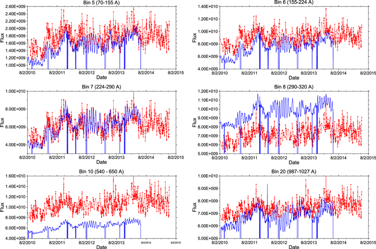
Figure 13. Photon flux in some of the 37 bins used by TIEGCM and TIMEGCM. The red traces and dots correspond to snapshots from the present synthesis; the blue traces were computed from SDO/EVE daily averaged measurements.
Download figure:
Standard image High-resolution image5.2.2. Physics-based Models of the Earth's Upper Atmosphere
A different approach to the modeling of the upper atmosphere is computer simulations of the physical processes in those layers. This is a complicated topic (way beyond the scope of our paper) whose SSI driving was until recently based on empirical models of the SSI, such as EUVAC, that use an F10.7 proxy scheme. Solomon and Qian (2005) also developed an empirical SSI model using the F10.7 proxy, with 37 wavelength bands with a combination of contiguous and, in some cases, overlapping wavelength bands that is used by the TIEGCM and TIMEGCM simulation models (e.g., http://www.hao.ucar.edu/modeling/tgcm/tiegcm1.95/release/html/) and also in other simulation models, e.g., CTIPe (Codrescu et al. 2012). In the first incarnation of the Solomon and Qian (2005) scheme, the photon flux in each of the bands assumed a linear scaling with F 10.7, but more recently, observational data are also used. It is beyond this paper to describe in detail the sources of these observational data; however, we mention that no available instrument covers the entire range of the 37 bins and that a combination, or composite, of data from various instruments and proxy models, sometimes based on broadband observations, is used for producing them. Also, the few spectrograph instruments currently operating do not have sufficient resolution to match the solar or Earth's upper-atmospheric lines, and suffer degradation that is not always accurately accounted for. Figure 13 shows the comparison between the current synthesis and the data from SDO/EVE for a few of the 37 bands. This figure shows some offsets between the two datasets, part of which are real data offsets, but others are not differences in the SSI but are due to the assembling of the bins that was based on 0.01 nm resolution in the current synthesis results and on 0.1 nm resolution data for SDO/EVE. The figure shows similar temporal behavior at least in the short wavelengths that did not suffer important degradation in SDO/EVE data and slightly different trends at longer wavelengths. It needs to be noted that synthetic data snapshots are indicated by symbols, while the SDO/EVE data correspond to daily averages. Also, in some periods, synthetic data are limited because of problems in obtaining and processing good-quality images; unfortunately, one of these periods occurred during the strong RM period around 2012 August. The short-wavelength channel of SDO/EVE suffered unrecoverable failure in the summer of 2014, and for this reason, some traces end at that point.
Note that the bin numbers indicated in Figure 13 start at 0 in our system, so they are offset by 1 with respect to other numbering systems, and for this reason, we also show the wavelength ranges. Bin 5 (7–15.5 nm) includes many hot coronal lines, which are affected by flares, and for the quiet-Sun the brightest lines are Ni x 14.5 and Ni xii 15.4 nm. In this band, many spikes in the synthetic data display the very variable nature of the snapshots in comparison with the much smoother EVE daily average. Bin 6 (15.5–22.4 nm) includes many large relatively cool coronal lines of Fe. The largest are Fe ix 17.1, Fe x 17.5 and 17.7, Fe xi 18.0 and 18.8, Fe xii 19.5, and Fe xiii 20.2 nm. The range of formation of these lines includes coronal holes to moderately active regions. The synthetic data are less spiky than in the previous bin but still shows the effects of snapshot fluctuations that are not present in the EVE daily averaged data. Bin 8 (29–32 nm) includes the very bright He ii 304 line and a number of upper transition region and coronal lines, such as Si xi 30.3, Mg viii 31.5, and Si viii 31.6 and 31.9 nm. The He ii 30.4 nm line in the present calculations is somewhat underestimated, but we plan to improve it soon. This explains the about 30% lower intensity and RM of the synthetic data. Bin 10 (54–65 nm) includes the chromospheric He i 58.4 nm line and bright transition region lines O iv 55.4 and Mg x 61.0 and 62.5 and the coronal line O vi 63.0 nm. In this band, EVE is lower and shows much less short-term variability than the synthesis but presents about the same long-term variability. Bin 20 (98.7–102.7 nm) contains the very important chromospheric+lower-transition region Lyβ line, and the EVE data might be contaminated by the O vi 103.1 nm line, which is nominally out of this band but is not resolved from Lyβ by EVE. Overall, the data from the synthesis and EVE compare well, but the comparison shows a few issues which, at least in part, can be attributed to the spectral resolution. However, much more important differences occur in the repeated λ intervals' bands—namely, the intervals ranging from 65 to 91.3 nm, each having more than one bin (see Solomon & Qian 2005). In these bins a comparison needs to be made between the N2 atmospheric absorption cross-sections at a much higher resolution than the 0.1 nm of EVE but a lower resolution than the 0.001 ∼ nm of SERFS. Apparently because of the spectral resolution issue, the synthesis distribution into the two or three bands that overlap is very different from the inferred distribution from EVE data, and this would translate in different height behaviors of the solar input at different atmospheric levels.
It is important to note that the spectral resolution used to produce our synthesized data is much better than the coarser resolution of the EVE data. This is particularly important for bins 9 and 10, because the He i 54.8 nm line is relatively broad and it seems that the EVE data distribute this line in these two bins, while our calculations do not. A similar situation could occur in other bins when important lines occur near the edges of the bins.
In our analysis of the comparison between our calculations and the EVE data, part of which is shown in Figure 13, we find that bin 8 contains the He ii 30.4 nm line and this line is computed as a factor of ∼0.75 of the values the EVE data indicate. However, EVE accuracy is at a fraction of ∼20% at this wavelength, and thus, the error in the calculation is comparable to the absolute accuracy of the EVE measurement.
We have also made scatter plots for most bins but can only show a couple of them in Figure 14, which illustrate the two types of behavior we found: (a) in the bins measured by the MEGS-A channel of EVE, we find the behavior illustrated in the figure for bin 6; (b) in the longer-wavelength bins measured by MEGS-B, we find the behavior of bin 20. The behavior of bin 6 can be summarized by an initial higher value of the relative difference between the computed and the EVE-measured value, a continuous decrease of this difference until about the end of the year 2011, and a constant difference afterward. Of course, at all times, important fluctuations occur because of the intra-day SSI variations that the EVE data average but our snapshot data preserve. The behavior of the scatter plot in bin 20 is very complicated, similar to a roller-coaster's. In the particular case of bin 21, the last one measured by EVE, our data value is about half of that of EVE, and the scatter is nearly constant and small. We do not elaborate further but note that the EVE instrument calibration degradation (included in the release 5) that we used could have some inaccuracies of the level of the long-term trends shown in Figure 14.
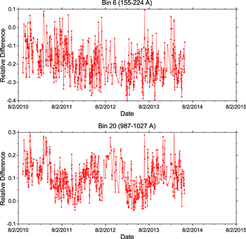
Figure 14. Scatter plot of some of the 37 bins used by TIEGCM and TIMEGCM. The values plotted are the relative differences between our calculations averaged for a day and the SDO/EVE daily averaged measurements. In most cases the computed averages are only from a single point.
Download figure:
Standard image High-resolution image6. APPLICATION TO THERMOSPHERIC NEUTRAL DENSITY AND IONIZATION
In this section, we show the results from a simulation of the upper atmosphere during 2012 that used synthesis UV SSI input in the 37 bins defined by Solomon and Qian (2005). The simulation was carried out with the CTIPe code (Millward et al. 1996, pp. 239–279), which was modified to use as input the present SSI synthesis results, and for reference, a simulation was carried out with the unmodified code, which uses the 37 bins' SSI proxy-based with the F10.7 index. Because the CTIPe code is "tuned" to run with the SSI input provided by the empirical model, the synthesis input was not used directly, but each of the 37 bins was scaled to match the empirical average values in the whole year. Other tests can be carried out, but for now this method permits a direct comparison with previous results, with no bias over the entire year. Otherwise, the CTIPe model would have to be completely re-tuned to accommodate the sometimes different magnitudes of the integrated heating and ionization effects. The presently used method is not ideal because it eliminates possible relative differences between the synthesized SSI and the empirical F10.7 proxy, in the various bands. Figures 15 and 16 show the year 2012 results for the neutral mass density and the peak electron density (NmF2) of the ionosphere F2 layer, respectively. The measured neutral density (black line in Figure 15) was obtained from the Gravity Field and Steady-State Ocean Circulation Explorer (GOCE) satellite and is orbit averaged at the satellite altitude ranging between approximately 240 and 290 km. In Figure 16, NmF2 was measured by an ionosonde at Chilton, England (51 5 N, 3594 E). The upper black trace is the averaged daily value calculated between 11 am and 12 pm, local time; the lower black trace is the averaged night-time value between 2 and 5 am. For reference a trace is shown that corresponds to the SSI in the 54–65 bin to distinguish the variations due to SSI from those due to geomagnetic inputs or to perturbations from below that are included in the CTIPe model.
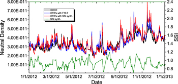
Figure 15. Neutral density measured by GOCE (in units of kg m−3). The plotted values are orbit averaged (black trace), compared with the values calculated by CTIPe for the F10.7 proxy SSI empirical model (blue trace) and the synthesis results' SSI (red trace). The synthesis SSI in the band 54–65 nm, which was linearly interpolated at intermediate times, is shown for reference (green trace).
Download figure:
Standard image High-resolution image
Figure 16. Ionospheric Nmf2 (in units of 1010 elec m−3), i.e., the maximum electron density in the F layer, from the Chilton ionosonde compared with the values calculated by CTIPe using the F10.7 proxy empirical SSI and the synthetic SSI. The synthesis SSI in the band 54–65 nm is shown for reference; at the snapshot times, it was linearly interpolated at intermediate times.
Download figure:
Standard image High-resolution image
In Figures 15 and 16, much of the short-term variability (over 1–5 days) is driven by geomagnetic activity and is driven in the same way in the two CTIPe simulations, with the synthesis and empirical proxy SSI. Differences in this response can occur because of a different atmospheric state in the two simulations. The main difference between the two model simulations is the multi-day variation (5–30 days), which is shown in the SSI 54–65 nm bin and displayed in the figures. In some cases, the use of the synthesized SSI improves the agreement of the simulation with the observation, but this is not universally true for the whole year. To quantify the agreement the root mean square error (RMSE) and the correlation coefficient (CC) were calculated between the output from the two CTIPe model runs and the observations of density and NmF2. The correlation with the GOCEdensity was better with the synthesized SSI case, 92% compared to 89% The correlation with the Chilton electron density was also slightly better with the synthesized SSI case, 62% compared to 61%, although the RMSE was slightly higher with the synthesized SSI case. The CC picks up the phases of the variations, and it is encouraging that the synthesized SSI run improves the response. The RMSE differences are less significant because the normalization procedure is not ideal. In the future a more appropriate method would be to use only one normalization value for all 37 bins so that the relative magnitudes of the fluxes in the different bands are kept and not forced to follow the F10.7 proxy model. As Figures 15 and 16 show, the simulation using the synthesis SSI input gave results comparable to but somewhat better than the run using the F10.7 proxy model. This demonstrates that synthesis data over extended periods are useful for the upper Earth's modeling with existing physics-based methods, even when they are tuned for proxy-based input. This indicates that developments in models that use the more accurate synthesis SSI input in a better way hold promise of better results than those shown here with a model whose photochemistry and heating are based on older data and not designed to take advantage of the very high resolution of our synthetic SSI.
Figure 16 also shows that a very significant issue with the CTIPe simulations of NmF2 occurs after 2012 October and lasts until the end of 2012. In that interval the measured index subsides from a local maximum at the beginning of 2012 October, but the simulated one increases rapidly and decreases but from the elevated value. Both calculations, F10.7 and the synthesis, stay close together and too high, but we caution that the synthesis SSI can be affected by its adjustment to the F10.7 proxy model because we do not see it in the original synthesized SSI data (also shown in Figure 16) any increase that could justify what the simulations show. This issue remains open for further investigation that is beyond the present paper.
7. DISCUSSION AND CONCLUSIONS
This paper has shown the capabilities of the combination of the three techniques SDID, SISA, and SRPM to integrate a processing chain that leads from images of the solar disk, presently SDO/AIA, to the complete SSI over the entire solar spectrum. In particular, UV SSI varies significantly and affects the upper Earth's atmosphere, which in turn affects the advanced technology currently used for space operations and communications. We have compared our synthesis results with existing indices and spectral observations, when available, considering both the irradiance absolute level and its variation during the 2010–2015 period. For these detailed comparisons, we picked indices that are used for empirical models of the Earth's upper atmosphere and the 37 spectral bands that are used for physical models such as TIEGCM, TIMEGCM, and CTIPe. These comparisons show generally good agreement, but there are a few bands where agreement should be improved. The issue of spectral resolution arises in some cases where the very high resolution of the synthesis data matches the fine spectra of the Earth's atmospheric absorption, but the observations so far cannot. The comparisons demonstrate the chain SDID–SISA using SRPM data for modeling the neutral density and ionization of the Earth's upper atmosphere by both empirical and physical models. An application is shown using the CTIPe code, which indicates our synthesis is useful for upper atmospheric modeling.
The results obtained for a part of the solar cycle SC24 reproduce the TSI trends observed by the SORCE/TIM instrument but are noisy, with a noise of ∼500 ppm compared to the cycle variation of ∼730 ppm observed in the period of this study. This is too noisy for accurate TSI reconstructions and is in part due to the low synthesis cadence, which is 1 point per day in most cases and sometimes has gaps, and largely to the poor quality of the SDO/AIA 450 nm channel. Similar noise is expected in the visible and IR SSI. A large improvement in the synthesized SSI can be expected from using good ground-based observations for the identification of sunspot umbrae and penumbrae, but they would have to be corrected for solar rotation due to the different timing of such observations and those from SDO/AIA.
The results for the EUV SSI show basic agreement with the SDO/EVE observations when the issues of the spectral resolution, absolute calibration uncertainty, and degradation correction uncertainty of SDO/AIA are considered. Also, for the EUV SSI, the low cadence of our synthesized data introduces significant "noise" due to intra-day variations of the SSI; some of this solar "noise" is even due to solar flares that are randomly captured in our synthesis but whose effect is much reduced in the SDO/EVE daily averages. Certainly, a faster cadence of synthesis, using more frequent images, would produce more representative daily averages and a more smoothly varying UV SSI. Even though the AIA instrument produces faster-cadence images at some wavelengths, the rate is particularly reduced for the 450 nm channel, which therefore would require correction for solar rotation and would not provide an advantage over using ground-based data.
However, even in its present limited form, our SSI nowcast can slightly outperform the old F10.7 proxy method, on which the CTIPe simulation code was based. However, it is clear that a new simulation code of the upper atmosphere is necessary for fully taking advantage of the synthesis capabilities and the spectral resolution that it brings to the field. Only this can effectively eliminate the need to normalize the synthesized SSI values to the empirical proxy method using the F10.7 proxy. This consideration also applies to all codes that use or derive from the TIEGCM or the TIMEGCM. While the limitations of the current physical simulation codes showed only in a few particular cases for the present solar cycle, SC24, of very small amplitude, it is likely that they will become more important in larger solar cycles in the future.
The SDID/SISA methods have been used for estimates of photoelectrons (Peterson et al. 2012) in the Earth's outer atmosphere. In addition to their use in the modeling of the Earth's upper atmosphere, other possibilities are enabled by the SSI synthesis methods described here. One is the forecasting of the SSI by considering observations of the far-side of the Sun, as shown in Fontenla et al. (2009b), and, more recently, observations of the Solar Terrestrial Relations Observatory (NASA). Also, a derivative of the SDID/SISA methods, Heliospheric Environment Solar Spectral Radiation (unpublished), allows one to compute the SSI at other planets, which can be used for modeling the atmospheres of other planets (Xu et al. 2015). Finally, the methods of SRPMv2 make it possible to model the atmospheres of stars other than the Sun and, using SISA, to infer the spectral irradiance on the atmospheres of exoplanets (Fontenla et al. 2016).
We acknowledge support from the Air Force Research Laboratory, under contract FA9453-14-C-0166. We thank the AIA team for the SDO/AIA data and the National Solar Observatory for their help with AIA data acquisition. We also thank the Global Ionospheric Radio Observatory (GIRO) and GIRO Principal Investigator Prof. B. W. Reinisch of the University of Massachusetts Lowell for making ionosonde data files available and Dr. Eelco Doornbos at Delft University of Technology and the European Space Agency for the GOCEdata.