


ABSTRACT
Neutron stars in low-mass X-ray binaries exhibit oscillations during thermonuclear bursts, attributed to asymmetric brightness patterns on the burning surfaces. All models that have been proposed to explain the origin of these asymmetries (spreading hotspots, surface waves, and cooling wakes) depend on the accretion rate. By analysis of archival RXTE data of six oscillation sources, we investigate the accretion rate dependence of the amplitude of burst oscillations. This more than doubles the size of the sample analyzed previously by Muno et al., who found indications for a relationship between accretion rate and oscillation amplitudes. We find that burst oscillation signals can be detected at all observed accretion rates. Moreover, oscillations at low accretion rates are found to have relatively small amplitudes ( ) while oscillations detected in bursts observed at high accretion rates cover a broad spread in amplitudes (
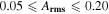 ). In this paper we present the results of our analysis and discuss these in the light of current burst oscillation models. Additionally, we investigate the bursts of two sources without previously detected oscillations. Despite the fact that these sources have been observed at accretion rates where burst oscillations might be expected, we find their behavior not to be anomalous compared to oscillation sources.
Export citation and abstract BibTeX RIS
1. INTRODUCTION
Neutron stars in low-mass X-ray binaries (LMXBs) accrete matter from their companion via Roche-lobe overflow. As the hydrogen- and helium-rich matter accumulates on the surface of the neutron star, it is compressed. For accretion rates  (where
  is the local Eddington accretion rate), the pressure increase leads to a thermonuclear instability which initiates unstable ignition of the accreted material (see the reviews by Bildsten 1998; Galloway et al. 2008). This results in a runaway event known as a type I X-ray burst, during which the material in the accretion layer is fused into heavier elements. To date, over 100 type I X-ray burst sources have been observed.3
One of the first discoveries obtained from observations with the Rossi X-ray Timing Explorer (RXTE) was that of thermonuclear burst oscillations (Strohmayer et al. 1996). These are periodic fluctuations in luminosity at a close to stable frequency that can arise during any phase of a type I X-ray burst. Burst oscillations have been observed in 18 sources to date, and for these sources the phenomenon is not necessarily detected in each burst.4
The fractional rms amplitude of the signal typically has a value in the range  . A characteristic property of burst oscillations is that the frequency of the signal tends to drift smoothly upwards by 1–3 Hz during the course of a burst, toward an asymptotic maximum that is nearly constant for each source (Muno et al. 2002a). The discovery of burst oscillations in the 401 Hz accretion powered pulsar SAX J1808.4−3658 (Chakrabarty et al. 2003) revealed that the oscillation frequency is close to the spin frequency of the pulsar in that system (Wijnands & van der Klis 1998). Although individual spin measurements have not been obtained for all oscillation sources, it is generally assumed that the oscillation frequency represents the spin frequency of the neutron star. The discovery of oscillations in SAX J1808.4-3658 confirmed the proposed theory that thermonuclear burst oscillations are caused by asymmetric brightness patterns on the burning surface of a neutron star during a type I X-ray burst.
The origin of the brightness asymmetries is an open question. Various models have been proposed that try to explain the underlying mechanism, and these can be divided into three main (non-exclusive) categories: hotspot models, surface wave models, and cooling wake models (see the review articles by Strohmayer & Bildsten 2006, p. 113; Watts 2012). Two factors on which the presence of a surface asymmetry depends are the ignition location of the burst, and the way that the flame spreads. It is generally assumed that the burst is ignited at one point on the surface of the neutron star, since the accretion time between two bursts is much longer than the time required for a thermonuclear instability to develop (Shara 1982). This makes it unlikely that the thermonuclear instability that initiates the burst arises everywhere on the surface at the same time, considering the level of thermal homogeneity that would otherwise be required. Spitkovsky et al. (2002) showed that the ignition occurs preferentially at the equator of the star rather than at higher latitudes, because of the reduced effective gravity force at this location. However, for specific accretion rates, or in cases of strong magnetic channeling, the preferred ignition latitude ( , where
  indicates the equator) is predicted be off-equatorial (Cooper & Narayan 2007; Maurer & Watts 2008) or even near the magnetic poles (Cavecchi et al. 2016). How the flame subsequently spreads determines how long an asymmetry can persist. An important question is whether the flame spread covers the whole surface or is confined to a smaller region. The flame spread depends both on the heat transfer mechanisms and the hydrodynamical effects involved. The two main factors that influence both the longitudinal and latitudinal propagation are the conductivity and Coriolis force (Spitkovsky et al. 2002; Cavecchi et al. 2013, 2015). Additionally, Cavecchi et al. (2016) showed that magnetic fields can significantly affect flame propagation.
In the hotspot models, it is assumed that the burst starts at one point on the surface of the neutron star (most likely at the equator) after which the flame spreads in all directions. If the hotspot arises on or close to the equator rather than at one of the rotational poles, the hotter region forms an azimuthal asymmetry and will be observed as an oscillation with a frequency close to the spin frequency of the neutron star. The growing hotspot can either engulf the entire star, after which the asymmetry is resolved, or it can be confined to a small region on the surface by various mechanisms (see Watts 2012, and references therein) such as Coriolis force confinement (Spitkovsky et al. 2002; Cavecchi et al. 2013, 2015) or magnetic confinement (Cavecchi et al. 2016).5 While spreading/confined hotspot models are supported by various aspects of the observations (Galloway et al. 2008; Watts et al. 2008; Cavecchi et al. 2011; Chakraborty & Bhattacharyya 2014), they cannot easily explain oscillations far in the tails of X-ray bursts, the absence of detected oscillations in some bursts, and the largest observed frequency drifts.
Surface wave models assume that the large-scale waves are excited in the outer layers of the neutron star (global modes) (Heyl 2004). These cause height differences in the burning layers, which can be observed as brightness patches. The waves are excited as soon as the initial hotspot starts to spread, and can persist after the flame has engulfed the entire surface of the star. The main difficulty with these models is that the predicted frequency drifts (which occur naturally as the surface layers cool) are too large compared to the observations (Piro & Bildsten 2005a, 2005b; Berkhout & Levin 2008). In addition, self-consistent models of mode excitation to sufficient amplitude are still required (although see Narayan & Cooper 2007).
In the cooling wake models, it is assumed that burst oscillations are caused by sequential cooling of different regions (for example, with the regions that first ignite being the ones that first start cooling.). If the cooling timescale is independent of position this cannot produce oscillations of sufficient amplitude: some degree of asymmetric (position-dependent) cooling would be required to reproduce the observed amplitudes (Cumming & Bildsten 2000; Mahmoodifar & Strohmayer 2016). Physical mechanisms that might lead to asymmetric cooling include transverse heat flows, or variations in the column depth at which the heat is released, which depends on the local depth of the accreted layer. An alternative, suggested by Spitkovsky et al. (2002), is that cooling wakes might drive zonal flows, which then induce atmospheric vortices (see also the discussion in Zhang et al. 2013). Note that cooling wake models cannot, of course, explain oscillations in the rising phase of bursts.
The proposed burst oscillation mechanisms depend at least in part on the (local) mass accretion rate onto the neutron star. The presence of unstable burning regimes, set by the local accretion rate, determines the ignition latitude (for example, whether ignition occurs on or off the equator), and hence whether or not the initial hotspot causes a brightness asymmetry. Ignition latitude in turn is an important factor in the various flame confinement models. For surface wave models, the accretion rate may be related to the question of whether or not the mode is unstable enough to grow to significant size (Narayan & Cooper 2007). Additionally, the accretion rate might be an important factor in the asymmetric cooling mechanism. Muno et al. (2004) showed that the detectability of burst oscillations is not determined by the properties of the X-ray bursts they occur in. Instead, they found that the oscillations seemed to occur preferentially when the source is in a higher accretion state. Additionally, they found that the upper limits on the amplitude of the oscillations appeared to be larger at high accretion rate, which led them to suggest that the amplitudes are attenuated at low accretion rate. However, the amount of data that was available at the time was insufficient to constrain the exact relationship between the two parameters.
To explain why the observed amplitudes seemed to be smaller at low accretion rate, Muno et al. (2004) considered whether the presence of an electron corona with optical depth  at low accretion rate could be the origin of the attenuation of the oscillations. Such a corona could scatter the photons from the neutron star surface, reducing the amplitude by a factor of two. However, as they pointed out, the electron corona is expected to be even more optically thick at higher accretion rates. Therefore, their suggestion requires that the geometrical configuration of the corona at high accretion rate be such that it prevents photon scattering. Since there are no indications of how such a change in configuration would be possible, this extra condition makes the suggested cause of oscillation attenuation rather unlikely.
In this research we investigate the type I X-ray bursts of six different burst oscillation sources observed with RXTE, with the goal of constraining the relationship between burst oscillation amplitude and accretion rate. We investigate the same sources as Muno et al. (2004), but extend the burst sample significantly compared to this research from 333 bursts to 765, such that for most sources more than twice the amount of bursts is analyzed. We compare our results to the expectations of various burst oscillation models, to gain insight on the thermonuclear burst oscillation mechanism. Additionally, we investigate the bursts of two LMXBs for which type I X-ray bursts have been observed over a wide spread of accretion rates, but for which to date no burst oscillations have been detected. Watts (2012) raised the question of whether or not these two sources might be anomalous in their behavior compared to the oscillation sources, because bursts from these two sources have been observed at an accretion rate limit above which most detections are found (Galloway et al. 2008). For these two sources, we carry out a similar analysis compared to the oscillation sources in order to determine upper limits on the oscillation amplitudes with the goal of understanding why no oscillations have been detected in these sources so far.
2. OBSERVATIONS
2.1. Telescope and On-line Data Catalogs
The burst sample that we analyze consists exclusively of observations from RXTE. Type I X-ray bursts are detected with the Proportional Counter Array (PCA). The PCA consists of five xenon-filled proportional counters, which are sensitive to photons with energies in the range 2–60 keV (Jahoda et al. 1996).
In this research we made use of information derived from bursts collected in the on-line RXTE catalog (Galloway et al. 2008) and the Multi-INstrument Burst ARchive (MINBAR), such as burst start times, spectral state of the source during the observation, and notes of any peculiarities of the bursts or observations. The MINBAR database contains information on all X-ray bursts observed with RXTE, BeppoSAX, and INTEGRAL.6 We collected the event mode RXTE data from the public NASA archive.7
2.2. Sources
We investigate the bursts of eight LMXBs. Six of these sources are confirmed burst oscillation sources for which some part of the data presented in the current paper was previously analyzed by Muno et al. (2004): 4U 1608-52, 4U 1636-536, 4U 1702-429, 4U 1728-34, KS 1731-26, and Aql X-1. The other two sources that we investigate are 4U 1705-44 and 4U 1746-37. These sources exhibit type I X-ray bursts, but have not been observed to show burst oscillations.
All sources are Galactic LMXBs, but the distances to them are not well constrained. Galloway et al. (2008) estimated the distances to 48 LMXBs, including the eight in our sample, from their PRE bursts, but since this requires knowledge of the mass, radius, and in particular the composition of the atmosphere of the neutron stars, the resulting distance ranges are rather large. Based on their spectral behavior, all sources are classified as atoll sources (Hasinger & van der Klis 1989), tracing out a wide range of accretion rates. Three of the investigated sources are transient sources; the remaining five sources are persistent X-ray emitters. Aql X-1 differs from the other sources, because this source is the only intermittent X-ray pulsar in the sample. It has shown one rare incidence of intermittent accretion-powered pulsations (Casella et al. 2008).
2.3. Burst Sample
In total we investigated 889 bursts from RXTE in this research. Initially, we obtained all available burst data of the selected sources from the public RXTE archive, in order to cover the largest possible accretion rate range and to obtain the highest possible statistical significance on any observable trend in the data. Subsequently, we discarded bursts from the sample based on the following criteria.
- 1.We eliminated all bursts that are marked with one of the following flags in either the RXTE or MINBAR database: e, f, g, h (Galloway et al. 2008). These flags indicate: (e) very faint bursts, for which only the burst peak could be observed, and no other parameters could be determined; (f) bursts that are either very faint or bursts for which there were problems with the background subtractions, such that no spectral fit of the burst could be obtained; (g) bursts that we only partly observed, resulting in an unconfirmed burst; (h) bursts that were not covered by the high time resolution data modes of the telescope. A total of 36 bursts was eliminated from the sample based on these flags.
- 2.We set a minimum background-subtracted burst count of 5000 counts within the first 16 s of the burst. This limit ensures that each burst can be divided in at least one full time bin (see Section 3.2.2). We excluded 57 bursts that did not meet this criterion from further analysis.
- 3.We determined bursts with gaps in the data that lasted for multiple seconds to be unfit for analysis. The RXTE catalog does provide a flag that indicates that the burst contains data gaps. However, we did not eliminate all bursts with this flag, but only those where the gap is so large that it affects the outcome of the burst analysis, which is the case for data gaps
 . The main problem with bursts with such large data gaps is that the gaps eliminate one or more full time bins (as defined in Section 3.2.2) from the burst. This means that there is a significant chance that the time bin with the strongest signal is lacking from the burst, which would affect the outcome of the analysis. We eliminated seven bursts from the sample based on this criterion.
 - 4.Bursts that are not fully observed by RXTE were eliminated from the sample. These coincide with the bursts with label g in the RXTE and MINBAR databases. However, there are bursts in the sample without this label for which (part of) the last phase before the start of the burst or the burst decay were not observed. Since we perform our analysis based on the 17 s before the start of the burst (to determine the background count rate) up to 16 s after, we eliminated three partially observed bursts that were not flagged with the g label by hand to ensure that all bursts are analyzed in a homogeneous way.

The properties of the burst sample are displayed in Table 1, including the number of bursts eliminated from the sample for each source. We list the number of bursts analyzed by Muno et al. (2004) for comparison to show that we do indeed significantly extend the number of analyzed bursts. No new bursts are available for KS 1731-26, since RXTE observations showed that the source returned to quiescent state in February 2001 (Wijnands et al. 2001a). We analyze for this source the same bursts as in the previous research. This way we can observe what kind of influences the small changes in analysis method have on the results. Table 1 also provides the frequency of the detected oscillations.
Table 1. Burst Sample
| Source |
 prev.1 prev.1 |

|
Eliminated |

|
|---|---|---|---|---|
| 4U 1608-52 | 28 | 56 | 9 | 620 |
| 4U 1636-636 | 124 | 381 | 42 | 581 |
| 4U 1702-429 | 18 | 50 | 1 | 329 |
| 4U 1705-44 | ... | 94 | 24 | ... |
| 4U 1728-34 | 104 | 176 | 15 | 363 |
| KS 1731-26 | 27 | 27 | 0 | 524 |
| 4U 1746-37 | ... | 30 | 8 | ... |
| Aql X-1 | 32 | 75 | 4 | 549 |
Note. Apart from the number of bursts in the initial sample of this research ( ), the number of bursts analyzed by Muno et al. (2004) is displayed as well (
 prev.: all bursts observed by RXTE up to 2003 August). The latter is displayed for comparison, to stress that we significantly extend the amount of analyzed bursts.
Reference. Muno et al. (2004).
Download table as: ASCIITypeset image
3. METHOD
3.1. Accretion Rate
The local mass accretion rate ( ) of accreting sources can be estimated from the persistent (between bursts) X-ray luminosity (
 ) of the source:

with R the radius of the neutron star,  the energy released per nucleon during accretion, and z the surface redshift (see Galloway et al. 2008).
For atoll sources, it is thought that a measure of accretion rate can be obtained from the position of the source in its color–color diagram (Hasinger & van der Klis 1989). This measure is determined by the spectral state of the source, the emission in hard X-rays (high energy) versus soft X-rays (low energy). Figure 1 shows the color–color diagrams from the eight investigated sources, using color data from the MINBAR database. The colors are determined from the spectral model: the ratios of integrated flux (based on the best-fit spectral model) are calculated in different energy bands. This is different from other approaches (e.g., Galloway et al. 2008) that calculate the ratios of counts in different energy bands rather than integrated flux. While the method used for MINBAR has a dependency on the spectral model, it has the advantage is that it is independent of the instrument used to obtain the data.

Figure 1. Color–color diagrams for each of the eight analyzed sources, taken from MINBAR. Each point represents the spectral state of the source during an RXTE observation. Colored dots are observations with one or multiple bursts; gray dots are observations without detected bursts. The SZ values (a measure of accretion rate) of the bursts are derived from their position relative to the SZ-curve (black curve). By definition, the upper right corner of the SZ-curve is assigned the value  and the lower left corner of the Z-shaped path
  as indicated in the figure.
Download figure:
Standard image High-resolution imageAtoll sources move along a specific path in a color–color diagram while the persistent luminosity increases (e.g., Homan et al. 2010). The spectral state of an atoll source is indicated by the value SZ. This value is obtained from the parameterization of the path that the source traces out (see Méndez et al. 1999; Galloway et al. 2008, for details of this method). By definition, the upper right corner of the path is assigned  and the lower left corner
  (see the color–color diagrams that were taken from the MINBAR database shown in Figure 1, in which we included for each source the SZ-curve with the assigned corner points). The SZ values of all other points in the diagram are extrapolated from these two. High SZ corresponds to high accretion rate. In this analysis we use SZ values from the MINBAR database and RXTE catalog.
Although it is still under debate whether or not SZ is the best measure of mass accretion rate, it has the advantage that it does not require estimates of the distance to the source, and the mass and radius of the neutron star. Some caution is required when comparing results from different stars since it might not necessarily be that a given SZ value for one source corresponds to the same accretion rate as for another. Spectral state was also used as a measure of accretion rate in the previous analysis by Muno et al. (2004), allowing us to determine the influence of a larger sample size on those results.
3.2. Data Analysis
We analyze each burst of the oscillation sources individually to determine whether an oscillation can be detected. We look for signals in the first 16 s of the burst with a frequency within 5 Hz of the known oscillation frequency ( Hz) to account for any frequency drift. Although in most cases the frequency drift is only 1–3 Hz (Muno et al. 2002a), larger drifts have been reported as well (Wijnands et al. 2001b). We use the range
  to be able to detect the largest possible drifts and to be consistent with the expected drifts from the proposed oscillation models. In the case of a detection (see Section 3.2.4), the fractional root mean square amplitude (rms amplitude) of the signal is computed. For those bursts in which we do not detect an oscillation signal that passes the detection criterion, we compute an upper limit on the rms amplitude.
In the following subsections the analysis method of bursts from the oscillation sources is described sequentially. The same method is applied to the sources without detected oscillations, but with a few adjustments since the spin frequency of these sources is unknown. The exact treatment of the bursts from these two sources is described in Section 3.3.
3.2.1. Burst Start Time and Background Count Rate
First we compute for each burst the burst start time (t0) and the background count rate. We estimate the background count rate using the count rate in the range 20–5 s prior to the approximate burst start time given in one of the databases. t0 is then defined as the time where the count rate equals 1.5 times the estimated background count rate. This ensures that all the burst start times are defined by the same criterion. Next, the true background count rate ( ) is defined as the average count rate in the range 17–1 s preceding t0. Muno et al. (2004) used the 16 s directly prior to the burst to compute the background. A time buffer of one second is kept between the burst start time and the range from which the background is calculated to ensure that the background is not overestimated in bursts with a slow rise.
3.2.2. Binning
Second, the first 16 s of the burst, ![$[{t}_{0}-({t}_{0}+16.0\,{\rm{s}})]$](https://content.cld.iop.org/journals/0004-637X/834/1/21/revision1/apjaa4a4bieqn25.gif) , is divided into non-overlapping time bins with 5000 counts each. We divided the bursts into time bins with an equal amount of counts to make the error bars on each measurement similar (Watts et al. 2005). Note that in a previous analysis by Muno et al. (2004) equal time bins were used, so that error bars later in the burst were larger (see discussion in Section 5.3). The number of time bins in our analysis thus depends on the strength of the burst and the underlying background. We use non-overlapping time bins to ensure that each bin is independent of the others. This makes it easier to compute the number of trials to obtain a signal (see Section 3.2.4).
, is divided into non-overlapping time bins with 5000 counts each. We divided the bursts into time bins with an equal amount of counts to make the error bars on each measurement similar (Watts et al. 2005). Note that in a previous analysis by Muno et al. (2004) equal time bins were used, so that error bars later in the burst were larger (see discussion in Section 5.3). The number of time bins in our analysis thus depends on the strength of the burst and the underlying background. We use non-overlapping time bins to ensure that each bin is independent of the others. This makes it easier to compute the number of trials to obtain a signal (see Section 3.2.4).
In each time bin we look for signals within 5 Hz of the known oscillation frequency. For each time bin we set up 10 frequency bins ( ), to obtain a frequency resolution of 1 Hz (equal to the resolution in Muno et al. (2004)). We thus create for each burst a two-dimensional grid of time-frequency bins in which we attempt to detect oscillation signals (see Figure 2 for a visualization of the grid).

Figure 2. Visualization of the time-frequency grid created to search for a burst oscillation. The first 16 s of a burst are divided into time bins with 5000 counts each. This means that the time bins are not equally broad in time space. For each time bin there are 10 frequency bins ranging from  to
to  , such that we look for signals within 5 Hz of the known oscillation frequency (
 ). The colors indicate which selection criterion applies to that bin. Blue = criterion 1: single bin detection (largest measured power of that time bin). Red = criterion 2: first bin detection. Green = criterion 3: double bin detections. Each green bin is an adjacent time or frequency bin to a blue bin, with which it forms a pair of double bins. Each blue bin has three adjacent bins which we use to look for double bin signals: both of the adjacent frequency bins and the next time bin.
Download figure:
Standard image High-resolution image3.2.3. Measured Power
We compute for each time bin the signal power for each of the 10 trial frequencies. We obtain the measured power for a signal with trial frequency ν by calculating the Z2 statistic (see Buccheri et al. 1983; Strohmayer & Markwardt 1999). The Z2 statistic is similar to a fast Fourier transform in the sense that it decomposes a signal into the sines and cosines that it consists of (see Equation (2)). This results in a power spectrum in which the power of the signal is plotted as function of frequency. The difference with a fast Fourier transform is that Z2 statistics does not require that the arrival times of the counts are binned. The Z2 statistic is defined as:

where Z2 is the measured power of the signal, n is the number of harmonics, Nγ is the number of counts in the time bin, and tj the arrival time of the jth count relative to some reference time. We only look for the first harmonic of each signal, so n = 1. By definition of the time bins  .
.
Using this statistic, we obtain a power spectrum for each time bin in which the power of the oscillation signals is plotted as function of the 10 trial frequencies. From such a spectrum one can easily determine at which frequency the signal is strongest. However, when frequency drifts between Fourier bins, the computed amplitude drops artificially (van der Klis 1989). We assume that the frequency of the oscillation is constant within each time bin and thus do not take into account frequency drifts within each bin.
3.2.4. Detection Criteria
For each individual time bin of a burst, we select the frequency bin with the largest measured power and determine whether or not the signal is considered a detection. We assume a Poisson noise process, for which powers in the absence of a signal are distributed as  with two degrees of freedom. This assumption is reasonable at high frequencies, but not at low frequencies where the red noise contribution due to the burst light curve envelope becomes significant. For this reason, we do not look for oscillation signals below 50 Hz in the two sources without previously detected oscillations. Based on the assumption for noise distribution, we can then determine the chance that any measured power is produced by noise alone. We can then set a threshold for the measured power above which we define a signal to be significant. We choose to set the detection criterion such that the chance that a signal was produced by noise is less than 1% when taking into account the number of trials for each burst
  . The number of trials in defined as the total number of time-frequency bins in which one looks for a signal; where
  with
with  the number of time bins and Nν the number of frequency bins.
The probability (Prob) that a measured signal with noise chance δ was produced by noise for N trials is given by:

Based on the detection criterion for each burst, we can define three criteria, similar to Muno et al. (2004), for which we determine a measured power to be a significant detection (see Figure 2 for a visualization of each criterion).
- 1.The chance that a measured power Zm was produced by noise is less than 7 × 10⁻⁵ in a single trial (), assuming that a burst will on average consist of 16 individual time bins, such that . This corresponds for 1% chance overall to a measured power criterion .
- 2.A signal occurring in the first second of a burst has a single trial chance probability. This probability results in a measured power limit . This detection criterion was introduced by Muno et al. (2004) as well. At the burst onset, the difference in brightness between burning and non-burning material is largest, and therefore oscillation signals would be expected to be largest in the burst rise (first second).
- 3.A signal distributed over two adjacent time-frequency bins has a combined single trial noise chance probability. We check this using the fact that this is similar to a measured power limit of the averaged signal in these two adjacent bins of . There is a significant chance that a signal does not peak exactly in one time-frequency bin, but is spread over multiple bins instead. Therefore, we select in each time bin the signal with the largest measured power and compute the noise chance of the signal that is spread over the selected time-frequency bin and one of three directly adjacent bins: the same time bin and one of two the adjacent frequency bins, or the same frequency bin and the next time bin. The chance that both bins consist of noise alone is given by the product of the noise chance probabilities of the two individual bins ().To meet the detection criterion of the burst, the single trial probabilities of the two bins ( and ) must satisfy the equation for . Using an approximation for given by Equation (4) (taking into account that N2 is reduced due to the fact that the second bin has to be selected from one of the three bins surrounding the first bin) yields the solution that adjacent bins must satisfy to meet the threshold burst probability .


Each of the detection criteria satisfies that, on average, an oscillation signal detected from a single burst has a 1% chance of being a false detection. If one considers each of the three detection criteria as individual trials, the noise probability would increase to a 3% chance that a detected oscillation is actually a false detection.
3.2.5. Signal Power
For each time bin we determine four different measured powers, all related to the frequency bin with the largest measured power: we determine the single bin measured power, which can either be in the first second (criterion 2) or at any other timespan in the analyzed part of the burst (criterion 1), and three double bin measured powers (criterion 3). However, each measured power consists of two components: the signal power and the noise power. To obtain the signal power and its uncertainty, we correct the measured power for the noise component. We do this using the method outlined in Section 2 of Watts et al. (2005) to compute the signal power of a given measured power and the number of harmonics.
The signal power is derived using the probability distribution pn of measured signals Zm for given signal power Zs:

where n is the number of harmonics (we always use n = 1), and I is a first kind modified Bessel function. The computational procedure provides a signal power and 1-σ errors.
3.2.6. Oscillation Amplitude
The oscillation amplitude of the signal in each time bin is computed from the signal power. As mentioned, there are five possibilities to pass the detection criteria: one from the first criterion, one from the second and three from the third. Per time bin we select from the five options the signal with the largest (averaged) measured power that passed the detection criteria. From the signal power of this oscillation, we compute the fractional rms amplitude of the oscillation ( ) using Equation (6).

The second term in Equation (6) is the factor that corrects for the background emission, where Nγ is the number of counts, and B is the estimated number of background counts in the investigated time bin ( and
and  , with
  the time width of the bin(s) over which the signal is considered). We calculate the 1-σ error on the amplitude using linear error propagation of the independent parameters, for which the standard deviations of Nγ and B are calculated as the square root of the considered parameter.
If none of the detection criteria are passed, an upper limit on the oscillation amplitude is determined with Equation (6) using the strongest (average) signal power (Z2s) from those that did not pass the detection criteria (non-significant signals). This definition results in upper limits that are defined in the exact same manner as the detections, such that the results from the detections can be compared to those of the non-significant signals. Note that Muno et al. (2004) defined the upper limit as the largest amplitude that could be obtained from the first five seconds after the start of the burst decay, because they argue that most detections are found in this phase. However, this upper limit is not necessarily based on the largest measured power found throughout the whole burst, and their non-detections are thus defined differently from the detections.
From the oscillation signals detected in a burst, we select the amplitude of signal with the largest signal power to compare with the results from other bursts (see Figure 3). We thus select one specific time-frequency bin for each individual burst. If no oscillation signals are found throughout an entire burst, we select the upper limit found for the signal with the largest non-significant signal power.

Figure 3. Result of the analysis of a burst from 4U 1728-34 with observation ID 95337-01-02-00, and t0 = 55474.175. The upper panel shows the burst itself, and the lower panel shows the limits of the time bins (dotted lines) and in each time bin the computed amplitude (asterisks with vertical error bars) or amplitude upper limit (triangles) in the case of a non-significant signal. In the upper panel the dotted line indicates the burst start time (t0) and the dashed lines represent the time bin in which the oscillation signal with the largest signal power Zs2 was found.
Download figure:
Standard image High-resolution image3.3. Analysis of Sources without Detected Oscillations
The two sources without previous detected oscillations, 4U 1705-44 and 4U 1746-37, should in principle be analyzed using the exact same method as the sources with oscillations, to be able to compare the results with the oscillation sources. However, the main problem is that for the two new sources, the oscillation frequency is unknown, such that we do not know in which 10 Hz frequency band to look for oscillations. What we do is to perform the analysis described above for every 10 Hz frequency band between  (the frequency windows on which we perform the analysis are thus defined as 50–60, 60–70, 70–80,...,2040–2050). The frequency upper limit is a frequency that encompasses the breakup speed of all current reasonable neutron star equation of state models (e.g., Haensel et al. 2009; Watts et al. 2015). Since the proposed oscillation mechanisms assume that the oscillation frequency is close to the spin frequency, the frequency range we trace has to be consistent with the allowed spin frequencies. As mentioned, we set a lower limit of 50 Hz, because below this limit the expected red noise signal is very large, which would make the analysis more complex. However, it should be noted that there is one confirmed burst oscillation source, IGR J17480-2446, with a frequency of 11 Hz (Cavecchi et al. 2011).
For each frequency window we analyze the data of the non-oscillating sources in the same way as the oscillation sources. However, since there are 199 frequency bands for which this method is applied, each burst of the non-oscillating sources is analyzed 199 times. This significantly increases the chance of detecting a noise signal. The signals that pass the detection criterion set for bursts that are analyzed only once, can therefore generally not be considered significant. Only when the signal is so large that it is still found to be significant when taking into account the total number of trials, can we conclude that the oscillation signal is likely not caused by noise (see Section 4.2).
The advantage of this method is that we can compare the results of any frequency window to those of the oscillation sources to determine whether or not the behavior of the non-oscillating source is anomalous. We select from both non-oscillating sources the results from the frequency band in which most signals are found that pass the detection criterion of the oscillation sources, since this is the best test of whether or not the source is anomalous.
4. RESULTS
4.1. Oscillation Sources
4.1.1. Accretion Rate Dependence of Burst Oscillation Amplitude
In Figure 4 the results of our analysis are plotted for each of the six oscillation sources. We plot from each burst the amplitude of the strongest oscillation signal as a function of SZ, which indicates the accretion state. Most of the detected oscillations were found to pass detection criterion 1 (149 out of 185 bursts with oscillations). We do not show any errors on SZ, because these are not yet available from the MINBAR database.

Figure 4. Accretion rate (indicated by SZ) dependence of burst oscillation amplitude for each of the six oscillation sources. From each analyzed burst we selected the signal with the largest signal power and plotted, depending on whether or not the signal passed the detection criterion, the corresponding amplitude (colored circles) or amplitude upper limit (triangles) as a function of SZ. This figure includes only the bursts with known SZ.
Download figure:
Standard image High-resolution imageOur results are consistent with Figure 2 from Muno et al. (2004). There are no deviations in the general distribution of the amplitudes of the detections as a function of SZ. Extension of the data sample seems to cause a larger scatter of the amplitudes rather than a confinement toward any fittable trend. A more specific comparison with Muno et al. (2004) shows that there does appear to be a small offset in the strongest signal of individual bursts; our amplitudes and upper limits tend to be slightly higher by 0.02–0.03. However, we do not detect a constant offset. We will discuss this difference in more detail in Section 5.3.
Figure 4 shows that most of the detected oscillations are found at high accretion rate;  (see also Table 2). However, at lower accretion rates, oscillations can also be detected. There does not seem to be a limit on SZ below which oscillations can no longer be detected, since for 4U 1636-536 and 4U 1728-34 detections are found in the bursts observed at the lowest SZ. Furthermore, all sources show similar behavior in oscillation amplitude as a function of
  this holds both for detected oscillations (see Figure 5) as well as for the amplitude upper limits of the non-detections (Figure 6). In Figure 5 (Figure 6) we plot the results of the detections (non-detections) of the individual sources on a background formed by the results of the detections (non-detections) from the other five investigated oscillation sources. The distribution of results from individual sources are consistent with the distribution of the general population of the other sources.

Figure 5. The behavior of the amplitudes of detected oscillations as a function of SZ for each of the individual sources (colored dots) compared to the results of detected oscillations from the other five sources combined (gray dots). Each source shows a similar trend in fractional rms amplitude as a function of SZ. Bursts with unknown SZ are omitted from this plot.
Download figure:
Standard image High-resolution image
Figure 6. The behavior of the amplitude upper limits of non-detections as a function of SZ for each of the individual sources (colored triangles) compared to the amplitude upper limits from the non-detections of the five other sources combined (gray triangles). Each source shows a similar trend in fractional rms amplitude upper limit as a function of SZ. Bursts with unknown SZ are omitted from this plot.
Download figure:
Standard image High-resolution imageTable 2. Detectability for High and Low SZ
| Source | Bursts with Detected Oscillations | |
|---|---|---|

|

|
|
| 4U 1608-52 | 0/27 | 8/20 |
| 4U 1636-536 | 7/141 | 73/196 |
| 4U 1702-429 | 0/6 | 35/43 |
| 4U 1728-34 | 4/76 | 36/55 |
| KS 1731-26 | 1/22 | 5/5 |
| Aql X-1 | 1/50 | 7/21 |
Note. Fraction of the bursts in which oscillations have been detected for high ( ) and low (
 ) accretion rates. Note that we omit bursts for which the SZ value is unknown.
Download table as: ASCIITypeset image
There is a trend in fractional rms amplitude as a function of SZ. The detections found at low accretion rate ( ) generally have low fractional rms amplitudes,
  . The amplitude upper limits of the non-detections are equally low. At higher accretion rate, the signals are found to have amplitudes over a broad spread;
  . A significant fraction of oscillation signals has a large amplitude:
  of the oscillations have an amplitude
  at
at  . The only exception is Aql X-1; in this source all six bursts with detected oscillation signals at
  are found to have amplitudes that satisfy
  . However, it should be noted that the number statistic is rather low.
The distribution in amplitude as a function of SZ is emphasized in Figure 7, which shows for each source (horizontal panels) histograms of the distribution of amplitudes for different SZ ranges (vertical panels). This figure includes the distribution of amplitudes of oscillations in combination with amplitude limits of non-detections. 4U 1636-536 and 4U 1728-34 have the largest burst sample and therefore the most reliable results. In the range  the amplitude distribution is strongly peaked around
  . On the other hand, at higher accretion rate (
 ) the peak of the distribution is still at 0.05, but the amplitude distribution is significantly broader due to the contribution of amplitudes of detected oscillations. Note that we tried but were unable to find a simple functional fit to the distributions.

Figure 7. Amplitude distribution for different ranges of accretion rate. The full range of accretion rates over which burst have been observed is divided into five equally spaced SZ bins (vertical panels). For each source (rows), a histogram of the spread in amplitudes of both the detections and non-detections is shown for each of the accretion rate ranges. The light areas in each histogram show the results of the combination of detections and non-detections, while the dark areas indicate the spread in detected oscillation amplitudes only. The peak of the full distribution seems to be around  at all accretion rates and in all sources, but as the accretion rate increases, the distribution significantly broadens. We note that each source has a different vertical axis and that this analysis only includes the bursts with known SZ.
Download figure:
Standard image High-resolution image4.1.2. The Dependence of Oscillation Detectability on Burst Phase
The proposed burst oscillation models differ in expected oscillation amplitudes and burst phases (rise, peak, or tail) during which oscillations can be detected. To be able to explain the results in the light of oscillation models, we also analyzed during which burst phase the detections are found using the obtained analysis figures of the individual bursts. We focus on the burst phase during which detections are found in bursts at both low accretion rates ( ) and in bursts at high accretion rates. At high accretion rate we specifically focus on oscillations signals with rms amplitudes that exceed
  , to find indications of what mechanism might cause such high amplitudes. The SZ limit is based on the results of sources 4U 1636-536 and 4U 1728-34, as there seem to be more oscillations, and those with higher amplitudes above this limit. Also, this limit is consistent with earlier studies by Galloway et al. (2008) who stressed that more detections were found for
  .
.
We discriminate between oscillations detected during the burst rise, peak, and tail. First we determine the maximum count rate of the burst using 0.25 s time resolution. The boundaries of the peak phase are then defined as the first and last time bin that exceed 90% of the maximum count rate. The burst rise phase starts at the burst start time and ends at the beginning of the peak phase, and similarly, the tail starts at the end of the peak phase and ends at the last analyzed time bin. This method is similar to the one described in Galloway et al. (2008). In cases where the selected 5000-count bin falls on both sides of one of the boundaries, we set the burst phase of the oscillation signal equal to the phase in which the signal was measured over the largest timespan.
4U 1636-536 has a significantly larger burst sample than all other sources, and is therefore the only source with a significant number of detections at different accretion rates. Determining the dependence of oscillation detectability on burst phase will therefore provide results with the highest significance for this source, but we present the results from all sources for completeness (see Table 3). Note that, in Table 3, we only present the burst phase results of the selected time bin (the one with the largest signal power) in each burst and do not consider oscillation signals with smaller signal powers detected in other burst phases.
Table 3. Burst Phase Analysis
| Source |

|

|
|||||||
|---|---|---|---|---|---|---|---|---|---|

|

|
||||||||
| R | P | T | R | P | T | R | P | T | |
| 4U 1608-52 | 0 | 0 | 0 | 2 | 1 | 3 | 1 | 0 | 1 |
| 4U 1636-536 | 4 | 3 | 0 | 10 | 3 | 38 | 17 | 1 | 4 |
| 4U 1702-429 | 0 | 0 | 0 | 5 | 5 | 17 | 0 | 0 | 8 |
| 4U 1728-34 | 0 | 1 | 3 | 4 | 7 | 10 | 7 | 3 | 5 |
| KS 1731-26 | 0 | 1 | 0 | 3 | 0 | 1 | 0 | 0 | 1 |
| Aql X-1 | 0 | 1 | 0 | 2 | 1 | 4 | 0 | 0 | 0 |
Note. This table shows how many signals were detected during either the rising phase (R), peak (P), and tail (T) of the burst. For each burst with oscillations, we only determine the phase of the strongest signal. We discriminate bursts observed at high ( ) and low accretion rate (
 ). In bursts observed at high accretion rate, we also distinguish oscillation signals with large amplitude (
 ) from low-amplitude oscillations (
 ).
).
Download table as: ASCIITypeset image
Oscillations have been detected in 81 of the 339 observed bursts from 4U 1636-536 in our sample. Seven of these bursts occurred while the source was in a low accretion state and all of the detections in these bursts were found either during the rising phase or peak of the burst. Moreover, considering all detected oscillations throughout each of these bursts, we stress that none of these seven bursts was found to have oscillation signals in the tail of the burst. From the 22 bursts observed at  that were found to have oscillation signals with
  , 18 were observed during the rising phase or peak of the burst.
Overall, for 4U 1636-536 two trends seem to be present: at low accretion rate ( ), oscillation signals are only found during the rising phase of the bursts or during the peak rather than the tail, and at high accretion rate most of the high amplitude oscillations (
 ) are detected in the rising phase. This second trend seems to be present in the bursts of 4U 1728-34 as well (see Table 3). In general most oscillations are detected at high accretion rate and have low amplitudes. These signals are most often found during the tail of the burst (in all sources). This trend is consistent with the results found by Galloway et al. (2008).
4.1.3. Oscillation Detectability as a Function of Accretion Rate
Since there are significantly more detections of oscillations found at higher accretion rate, we decided to look at the detectability of the oscillations as a function of accretion rate. We combined the results from all sources, divided the SZ range [0.6–2.8] into non-overlapping bins with 0.1 width, and determined in each bin what fraction of the burst contained detected oscillation signals. The oscillation detectability is defined as the number of bursts with oscillations in one SZ bin, divided by the total number of bursts in the considered bin. We used the combined results rather than those of individual sources to increase the number of bursts per bin and with that the significance of each point. Combining the results is justified by the observation that the behavior of each of the oscillation sources was found to be similar as a function of accretion rate (Section 4.1.1).
Figure 8 shows the oscillation detectability as function of SZ. For  the oscillation detectability is smaller than 10%. Moreover, for
  no oscillations were detected. However, because of the low number of bursts in this range (note that in Figure 8 the number of bursts in a specific SZ range is indicated by the size of the purple circles), these points cannot be considered to be statistically significant. For SZ values larger than 1.7, the oscillation detectability significantly increases. A steep increase of oscillation detectability as a function of accretion rate can be observed for
  . The oscillation detectability goes up to 85% for
  . For the highest accretion rates (
 ) the detectability is found to decrease, but so does the significance.

Figure 8. Oscillation detectability as function of accretion rate determined from all bursts of all sources combined. The detectability is defined as the fraction of bursts with detections within non-overlapping SZ bins with 0.1 width. The size of the purple circles indicates the number of bursts in the SZ bin, with larger circles containing more bursts. Note that the size of the circle does not indicate significance. Computation of formal error bars on the number of bursts with oscillations is not straightforward since we have three different detection criteria (see Section 3.2.4) based on distributions of powers, so we have not attempted to compute these. The figure shows that while the detectability is low at the lowest accretion rates, there seems to be a steep increase in oscillation detectability for SZ values larger than 1.7. Note that we omit bursts for which the SZ value is unknown.
Download figure:
Standard image High-resolution image4.2. Sources without Previously Detected Oscillations
For the two sources without previously detected oscillations, 4U 1705-44 and 4U 1746-37, we looked for signals within each 10 Hz frequency band between 50 and 2050 Hz. We thus carried out the analysis of all bursts for 199 different frequency bands. For both sources we selected the results of the frequency band with the most positive outcome based on the number of signals that pass one of the criteria for the oscillation sources and the strength of the corresponding signal power. We do this because if the properties of the signals in this band (the best candidate for a detection) are anomalous compared to the sources that do exhibit burst oscillations, then the other bands will be even more so.
In this section we refer to signals that pass one of criteria for a single searched frequency window (these are the criteria for the oscillation sources) as pass signals. These pass signals are not detections, because for the two sources without previous detected oscillations we apply our analysis method to 199 frequency windows. This means that if we take into account the number of trials for these two sources, none of the signals can be considered significant. The oscillation signal of a single bin detection (detection criterion 1) would have to be as strong as  for 4U 1705-44 and
  for 4U 1746-37 in order to be considered significant.
4.2.1. 4U 1705-44
From 4U 1705-44 a total of 70 bursts were analyzed after the burst selection process (Section 2.3). In the frequency range ν = 1800–1810 Hz we measured four pass signals. This range was selected as most positive and therefore we present the results obtained from this frequency band (see Table 4 for the three frequency bands with the best results). The largest signal power among the four pass signals is  .
.
Table 4. Frequency Analysis for 4U 1705-44
| Rank | ν Band | Pass | Max 
|
Significant |
|---|---|---|---|---|
| (Hz) | ||||
| 1 | 1800–1810 | 4 | 22.7 | No |
| 2 | 270–280 | 3 | 20.8 | No |
| 3 | 1820–1830 | 3 | 13.7 | No |
Note. None of the signals meets the detection criteria and we thus do not detect oscillations for any frequency
Download table as: ASCIITypeset image
Figure 9 shows the results of the fractional rms amplitude as a function of SZ (upper left panel), as well as an overplot of the results on a background of the results from all oscillation sources (lower left panel). From the upper panel one can observe that very few bursts are observed at the highest accretion rates. The lower panel shows that the distribution in fractional rms amplitude as a function of accretion rate of the observed signals seems to be similar to those of the oscillation sources.

Figure 9. Upper panels: fractional rms amplitude as a function of accretion rate (SZ) for the two sources without previously detected oscillations. Since the spin frequency both of these sources is unknown we plot the results for the frequency range in which the most significant results were obtained. None of these results are detections. Lower panels: results of the non-oscillating sources (purple: 4U 1705-44, and orange: 4U 1746-37) plotted on a grey background formed by the results of the oscillation sources. In all panels, dots indicate pass signals and triangles represent upper limits.
Download figure:
Standard image High-resolution image4.2.2. 4U 1746-37
We analyzed 22 bursts of 4U 1746-37 that passed the burst selection, and found in all frequency bands for which the analysis was carried out no more than one pass signal. We present the results from the frequency range ν = 1880–1890 Hz, because the pass signal in this range has the largest signal power;  (see Table 5). The upper right panel of Figure 9 shows the fractional rms amplitudes as function of SZ. A notable observation from this figure is that more than half of the observed bursts at high accretion rate are found to have upper limits larger than
  , while in all oscillation sources the upper limits are rarely found to be this large. For most bursts of the oscillation sources, the upper limits are lower than the typical amplitudes of detected oscillations at that accretion rate, because in general a weak signal has a very low amplitude. Other than that, the selected signals from the observed bursts of this source show no abnormalities in distribution of amplitudes as function of accretion rate (lower right panel of Figure 9).
Table 5. Frequency Analysis for 4U 1746-37
| Rank | ν Band | Pass | Max 
|
Significant |
|---|---|---|---|---|
| (Hz) | ||||
| 1 | 1170–1180 | 2 | 24.4 | No |
| 2 | 1970–1980 | 1 | 24.3 | No |
| 3 | 1240–1250 | 1 | 22.8 | No |
Note. None of the signals meets the detection criteria and we thus do not detect oscillations for any frequency
Download table as: ASCIITypeset image
4.2.3. Statistical Significance
To determine whether or not the two new sources are anomalous compared to the oscillation sources, we tried to obtain the probability of finding a distribution of pass signals as low as we did. Initially we tried to do this by fitting the distribution of amplitudes as function of SZ observed for the oscillation sources. However, we were unable to find a simple function that would adequately fit the data (primarily due to the broad spread in amplitudes at high accretion rate). Then we fitted the distributions of amplitudes in different SZ bins (Figure 7) with several functions (see Section 4.1.1).
Subsequently we applied a more robust method to obtain a value for the probability of the amplitudes found for the two sources without previously detected oscillations. Since 4U 1636-536 has the most bursts and the largest amount of bursts with oscillation signals, we set this source as a model distribution. Most detections are found at high accretion rate ( ) and the amplitudes of the oscillations are higher. Larger fractional rms amplitudes indicate stronger signals, and we thus expect to find the most, and the most significant, results at high accretion rate. We determine how likely it is that the signals that passed any of the detection criteria, observed in bursts at high accretion rate of the two non-oscillating sources, have amplitudes as low as they do. We use the distribution formed by the detected oscillations in the bursts from 4U 1636-536 to determine this probability. First, we determine how many pass signals (
 ) are found for each of the two non-oscillating sources at
  and the largest amplitude (
 ) among these pass signals. Then we randomly pick
  amplitudes of the detected signals with
  of the model distribution, and determine whether or not the condition that all
  amplitudes satisfy
  is met. We repeat the sampling process 10,000 times and determine how often the condition is satisfied. We find that for 4U 1705-44 there is a 15% chance of finding oscillation amplitudes as low as those observed. For 4U 1746-37 this chance is 95%. We conclude that neither source is anomalous given the limitations of current data.
5. DISCUSSION
5.1. The Accretion Rate Dependence of Burst Oscillation Amplitude
From the six oscillation sources three general trends were observed. First, oscillations can be found at all accretion rates: there are no SZ ranges for any source in which oscillations are absent to a degree that can be considered statistically significant. Second, most oscillations are found at high accretion rates. For  oscillations are detected in less than 10% of the bursts, while at higher accretion rates the fraction of bursts with detected oscillations rises to 85% at
  . Third, the oscillations detected in bursts at low accretion rate have low amplitudes,
  , while the oscillations in bursts at higher accretion rate have a broad distribution of amplitudes (
 ). Detection limits vary somewhat from burst to burst, but in general amplitudes
  would not be detectable. All of these observations are consistent with the results from Muno et al. (2004). Extension of the data sample emphasized the similarities in amplitudes as a function of SZ between the different sources and allowed us to determine absolute values for oscillation detectability at different accretion rates.
We set out to determine how the oscillation amplitude changes as a function of SZ. We were not able to fit a smooth function through the detected amplitudes; the scatter is too large. However the distribution is also inconsistent with a step function: there is no SZ limit below which the oscillation mechanism simply switches off.
We also investigated two non-oscillation sources with bursts at high SZ. We found that the non-detection of oscillations in these sources does not contradict the trends observed in the oscillation sources. 4U 1705-44 has very few observations at high SZ, reducing the chance of detecting oscillations. 4U 1746-37 has a larger sample of bursts at high SZ, but the distance to this source is much larger. While the other seven investigated sources have estimated distances <8.2 kpc, the distance to 4U 1746-37 is thought to be in the range 13–25 kpc (Galloway et al. 2008). The fact that the bursts are fainter as a result reduces the chance of detecting oscillations. We conclude that neither source shows anomalous behavior.
5.1.1. Burst Oscillation Amplitudes in Light of Current Theories
Surface mode patterns cannot give amplitudes as high as hotspot models, since in the latter the bright spot can be restricted, physics permitting, to a smaller region of the star (either as it spreads from the ignition point or due to some mechanism like magnetic confinement). Obtaining amplitudes  with any of the suggested models is certainly feasible, but obtaining amplitudes as high as
  with surface mode models will be more challenging. For canonical cooling wake models, amplitudes are predicted to be low,
  , while for asymmetric cooling wake models, amplitudes can be as large as
  , depending on the ignition latitude (Mahmoodifar & Strohmayer 2016). An overview of the maximum amplitudes predicted for each model is given in Table 6, along with other relevant phenomena predicted for each model.
Table 6. Summary of Model Predictions
| Hotspot | Surface Waves | Cooling Wakes | |
|---|---|---|---|
 max. max. |
0.2 | 0.1 | 0.2a |
| Burst phaseb | R Pc Tc | T | T |
| SZ dependence | - Ignition latitude might | - Signals might only be able | |
| depend on SZ | to grow to detectable size at | ||
| high SZ | |||
Ignition latitude ( ) dependence ) dependence |
- If stationary, max.  lower lower |
- Max.  decreases with decreases with |
|
for high 
|
increasing 
|
||
| - Coriolis force confinement | |||
more effective at high  , , |
|||
reducing low  amplitudes amplitudes |
|||
Notes. Empty boxes indicate that, at present, there are no clear model predictions.
aArms up to 0.2 can only be obtained for asymmetric cooling wake models. bR—rising phase, P—peak of the burst, T—burst tail. cA hotspot can only produce oscillations during the peak and tail of the burst if the hotspot is confined.Download table as: ASCIITypeset image
What then do the data require us to explain in terms of accretion rate dependence? As the accretion rate rises, the mechanisms operating must permit higher maximum amplitudes, but also allow the possibility of the amplitude remaining low, since we see bursts with amplitudes that never get much above the detection limit even at high accretion rate. What then is the expectation in this regard for the different proposed mechanisms?
For the spreading hotspot model, the most obvious dependence on accretion rate should come if ignition does indeed move off-equator to higher latitudes as the accretion rate increases (Cooper & Narayan 2007). This is due to variations in local accretion rate from rotational effects, which can cause burning to stabilize at the equator before it stabilizes at higher latitudes. This should occur for a relatively narrow band of accretion rates, but recall that it is not straightforward to map SZ to an absolute accretion rate. The predicted effect on amplitude, however, is not immediately clear. All other things being equal, a stationary hotspot at higher latitudes should give a lower amplitude than a hotspot on the equator (Muno et al. 2002b). However, the speed at which the flame spreads from the ignition point will also have an effect. Coriolis confinement is more effective off-equator (Spitkovsky et al. 2002; Cavecchi et al. 2013, 2015) so an equatorial hotspot can be quickly wiped out as the flame spreads, reducing amplitude. There may even be multiple phases of on- and off-equator ignition as the accretion rate changes, at the transition phases between different burning regimes (Maurer & Watts 2008). The intrinsic dependence of flame speed on accretion rate (as e.g., the properties of the ocean change), and the dependence of stalling mechanisms such as magnetic confinement (Cavecchi et al. 2016) on accretion rate, are not known.
So is the hotspot model consistent with our observations? Let us start with the overall rise in oscillation amplitudes. The very simplest model, where ignition location moves off-equator as accretion rate increases and flame spread does not change, would not explain the large rise in maximum amplitude, since the amplitude should fall. For the spreading hotspot model to fit the data, either flame spread must slow significantly as ignition moves off-equator due to Coriolis effects (as predicted), or ignition is actually moving back on-equator at high accretion rates, due to the presence of multiple burning regimes. The alternative is that some stalling mechanism becomes more effective as the accretion rate rises. What about the spread in amplitudes seen at higher accretion rates? In the simple spreading hotspot model, ignition latitude and flame spread speed from that point should vary monotonically with accretion rate. It is therefore hard to see how such a broad spread is possible if this is the only mechanism in operation, unless ignition location depends on other factors as well.
Predictions for the accretion rate dependence of surface mode amplitudes center around the need to excite the oscillations to detectable amplitudes. Narayan & Cooper (2007) have argued that there is a nuclear burning driven instability mechanism that would operate to pump mode amplitudes primarily in helium-dominated bursts, which occur preferentially at higher accretion rates. If this is correct, surface mode amplitudes should rise as the accretion rate increases. This matches the observation of a general rise in amplitude, although surface mode models would still struggle to explain the very highest amplitudes seen at the highest accretion rates. Given that there are mechanisms that could also suppress surface mode amplitudes again e.g., in bursts where a large convective layer develops (Cooper 2008), surface mode models could also viably explain the lower amplitudes seen in some bursts as well.
Our conclusions at this stage are rather tentative. Hotspot models can in principle give rise to the highest amplitudes seen, and it is possible to explain the overall rise in the envelope of the amplitude distribution with accretion rate provided that the flame spread speed varies strongly with latitude (for simple expectations of the change in ignition latitude with accretion rate). However, this simple model on its own would struggle to explain the fact that at similar accretion rates there are also bursts that do not show high-amplitude oscillations. Perhaps ignition location varies more than expected, or we are seeing the effects of a stalling mechanism, or flame spread speed simply varies much more than indicated by current studies. Alternatively we are seeing a second mechanism coming into play at higher accretion rates, to give the lower-amplitude population. In this scenario the high- and low-amplitude oscillations at high accretion rate would be caused by two different mechanisms. Surface mode models, which can explain amplitudes up to about 0.1, would fit well in this regard since instability mechanisms that might pump them to detectable amplitudes are only expected to kick in as accretion rate rises. We cannot comment on the cooling wake model of Mahmoodifar & Strohmayer (2016) since at this stage there are no concrete predictions for accretion rate dependence against which to compare.
5.2. The Accretion Rate Dependence of Oscillations at Different Burst Phases
To shed more light on the mechanisms at work, we analyzed the burst phases in which oscillations are detected for bursts at different accretion rates. Figure 10 shows for each burst in which oscillations were detected, the amplitude of the strongest oscillation signal as function of SZ, as well as the burst phase in which this signal was detected. The left panel shows these results for 4U 1636-536 (the source with the largest burst sample), and the right for the remaining five oscillation sources combined.

Figure 10. Left: result of the burst phase analysis for bursts with detected oscillations in 4U 1636-536. We show for each burst in which an oscillation was detected the amplitude as function of accretion rate, while the symbol indicates whether the oscillation was detected during the rising phase (black stars), peak (red hexagons), or tail (gray dots) of the burst. The vertical line indicates the separation between high and low SZ, while the horizontal line indicates the separation between high and low amplitude. Note that the symbol indicates only the burst phase in which the strongest signal was found. Right: same as left panel, but for the detected oscillations in 4U 1608-52, 4U 1702-429, 4U 1728-34, KS 1731-26 and Aql X-1 combined. Since amplitudes of different sources are combined in this figure without taking into account any inclination effects, we do not distinguish high and low amplitudes.
Download figure:
Standard image High-resolution imageTaking the sample as a whole, the maximum oscillation amplitude can occur, for any SZ, during any phase of the burst. The very largest amplitudes seen, for a given SZ, are always found in the rise. However this latter finding depends entirely on the inclusion of 4U 1636-536 in the sample. At the lower end of the maximum amplitude distribution envelope, all burst phases are represented (the picture for  appears to show some separation, but there are too few bursts with oscillations here to draw reliable conclusions). Interestingly, however, maximum amplitudes at any specific burst phase show the same general trend: the maximum of the envelope that can be reached rises as the accretion rate increases, while the lower end of the envelope remains at the detection threshold.
How do these observations fit within the context of current theoretical expectations? A spreading hotspot is expected to cause oscillations during the rising phase of the bursts only, since the brightness asymmetry disappears as soon as the flame has engulfed the entire surface of the neutron star (Chakraborty & Bhattacharyya 2014). A stalled hotspot would cause detectable signals in all phases of the bursts (rise, peak, and tail), as long as it is offset from the rotational pole. Since surface waves require time to grow to significant size, perhaps comparable to the duration of a burst (Narayan & Cooper 2007), surface wave oscillations are expected in the tails only. However, it is unknown when in the tail these oscillations are expected to be strongest. Cooling wake oscillations are only able to explain burst tail oscillations. Mahmoodifar & Strohmayer (2016) calculated the expected amplitude evolution during a burst and found for canonical cooling wakes that the amplitudes are strongest ∼1 s after the peak of the burst, after which they would decay. For asymmetric cooling wakes the amplitude evolution of the oscillation signal is expected follow a smooth parabolic evolution, with a maximum ∼5 s after the peak of the burst. The exact amplitude evolution depends, among other factors, on the ignition latitude. An overview of the burst phase in which oscillations are expected for each model can be found in Table 6.
The fact that the very largest maximum amplitudes ( ) are seen in the rise is consistent with the idea that these are caused by a (spreading) hotspot with an appropriate observing geometry. The lower-amplitude oscillations are consistent with any of the models put forward, although as stated in Section 5.1.1 modes would have to be excited much more quickly than current models predict if they are to explain rise phase oscillations. However our data do now pose a strong constraint on all models. The mechanism(s) in operation must (1) be capable of permitting higher-amplitude oscillations at all burst phases as the accretion rate increases and (2) still permit the generation of low-amplitude oscillations at all burst phases. Whether this can be achieved with one mechanism alone is an interesting question.
5.3. Method Effects and Assumptions
In this research we followed the method from Muno et al. (2004) for the analysis and detection of oscillations. There are, however, two main differences between our methods. First of all, Muno et al. (2004) used one-second time bins, while we use time bins with an equal number of counts (5000 counts per bin). For a typical burst, the bins will on average have a width of one second. However, for fainter bursts, the time bins grow in width. The disadvantage of this method is that for broad bins, the signal might drift in frequency within the bin, making the signal hard to detect, even though we also look for signals in overlapping frequency bins. Also, the number of bins significantly falls for bursts with low count rate, decreasing the chance of a detection as the number of trials for the burst is lower. We excluded bursts for which the average count rate was too low to have multiple bins of reasonable width, to reduce the number of bursts for which it is very likely that no oscillations are found due to the methodology. The benefit of this method is that, since the amplitude error depends on the number of counts in a time bin, all errors will have the same contribution of the uncertainty in counts per time bin.
As mentioned in Section 4.1.1, our oscillation amplitudes tended to be slightly higher (∼0.02–0.03) compared to the results of Muno et al. (2004). However, an offset was only present in some bursts and this offset is not constant. We checked the results when using one second time bins, and found no deviations in the amplitudes from Muno et al. (2004) in that case, indicating that the observed differences in amplitudes are caused the difference in the definition of time bins. A comparison of individual bursts showed that many of the 5000-count bins in our research are smaller than one second, especially near the peak of the burst. As a result, the selected signal of a burst often originates from a bin smaller than one second. Within smaller time bins, the strength of the oscillation signal will be less affected by frequency drifts. Consequently, the oscillation signal will be stronger. It should be noted that for bursts where the width of the time bins deviates from the assumed one second, the total amount of bins increases. This affects the probability of a signal being caused by noise. We checked the number of time bins per burst after the analysis, and corrected signals that were wrongly classified due to the standard probability calculation (based on 16 time bins per burst) by hand.
A second difference from the method of Muno et al. (2004) is that they select the upper limit of a burst oscillation as being the signal with the largest non-significant amplitude from the first five seconds after the start of the burst decay, while we select the signal with the largest non-significant power throughout the whole burst. This upper limit is computed by the same method used to obtain the oscillation signal from a single burst, such that amplitude upper limits and detected oscillation amplitudes can be compared with each other.
We checked that a similar trend can be found in the measured powers as in the rms amplitude as function of SZ. This indicates that the results do not depend on the method that we use to convert measured power into signal power and consequently into rms amplitude. A recent study showed that the persistent luminosity during a burst is variable, while we estimate a constant background from the pre-burst emission (Worpel et al. 2015). This would influence the background correction that we apply while obtaining the rms amplitude. The effect found by Worpel et al. (2015) is a factor of a few increase in persistent emission during the rise and peak of the burst. Consequently, if the background increase was taken into account, the measured burst oscillation amplitudes during the rise and peak of the burst would have been larger (Equation (6)). Burst tail oscillations would be unaffected. Future study would be required to determine whether such changes in persistent emission would be sufficient to give rise to the trends that we observe without requiring any change in the burst oscillation mechanism.
In this research we chose to use non-overlapping time bins and to select from each burst the signal with the largest power. However, we also could have taken the average amplitude of the oscillation signal over the whole burst instead. Another method that is often used for analysis of burst oscillations is to determine the dynamical power spectrum of each burst, which requires the use of overlapping time bins. This method has the advantage that the frequency drift can be determined.
Additionally, we chose to use the SZ value as measure of accretion rate. It should be pointed out that it is still under debate whether or not this is indeed the best measure of accretion rate. One might also consider using γ, the fraction of persistent flux compared to the Eddington flux.
Any possible effects of rotational and binary inclination on the determined oscillation amplitude are not taken into account. One may assume that as a consequence of mass accretion, the rotational and binary inclination are aligned (Hills 1983; Bhattacharya & van den Heuvel 1991; Guillemot & Tauris 2014), such that the effects of rotational and binary inclination can be discussed together. None of the sources are known dippers, which limits the binary inclination angles to (typically)  (see e.g., Galloway et al. 2016). Inclination is expected to affect the observed amplitudes originating from hotspot oscillations, depending on the ignition latitude. Muno et al. (2002b) showed that for a stationary hotspot, the maximum observed amplitude is observed for inclination angle between the observer and the neutron star spin axis:
  . Detailed analysis of possible correlations between the inclination angle and amplitudes is beyond the scope of this paper. Once strong constraints on the inclination angle of all systems are obtained, one can consider the possible effects on our results.
We estimated confidence limits on the maximum rms amplitude by assuming that the measured amplitudes are distributed uniformly between zero and some maximum value,  . This assumption must be viewed with caution, both because the observed distribution is far from uniform (e.g., Figure 7), and also because arbitrarily small amplitudes cannot be measured, due to the detection threshold, so that the effective minimum amplitude is
  . Nevertheless, the largest impact on the probability density function of
  is the measurements with the largest amplitudes. We find for individual sources that the highest-probability value of
  was between 10 and 17%, with the extreme sources being Aql X-1 and 4U 1636-536, respectively. For the entire sample, the inferred
  , with a 95% upper limit of 15.4%
Finally, in this research we only investigated the bursts from six of the 17 confirmed oscillation sources and two of the 87 type I X-ray burst sources without previously detected oscillations. One may wonder if the results are not biased because we only selected a subsection of the available sources. Preferably, we would investigate all oscillation sources, but the main problem with is that in those other sources usually very few bursts with oscillations have been observed and typically only a small range of accretion rate. This impedes the construction of a color–color diagram from which SZ values can be obtained. Using a different measure of accretion rate would circumvent a possible bias that could be present due to the fact that we select only sources that exhibit a large variation in accretion rate.
For sources without previously detected oscillations, a similar argument holds. It would indeed be better to investigate all sources without previously detected oscillations, but we chose these two because a significant number of bursts was observed from them over a broad range of accretion rates, and specifically because they were observed at  where most oscillations are detected. The sources were therefore prime candidates for the detection of oscillation signals, and what we constrained is that at least these sources do not seem to be anomalous in their behavior as far as can be observed. Additional monitoring of the bursts of the remaining non-oscillating sources is suggested for further research.
6. CONCLUSIONS
We have analyzed 765 type I X-ray bursts of six different LMXBs that are all known to exhibit thermonuclear burst oscillations. The goal of this research was to investigate the accretion rate dependence of burst oscillation amplitude in order to gain insight on the mechanism that causes the asymmetric brightness patterns on the burning surfaces of accretion neutron stars that underlie the burst oscillations. Additionally, we analyzed the bursts of two sources without previously detected burst oscillations (124 bursts in total) that have been observed over a broad range of accretion rates. These two sources are observed at accretion rates  , a limit above which most oscillations are detected. We have found the following results.
- 1.Oscillations can be detected at all accretion rates; there is no evidence for a cutoff in accretion rate below which oscillations are no longer detectable.
- 2.Significantly more detections as a fraction of number of bursts are found at high accretion rate than at low accretion rate. This confirms earlier results by Muno et al. (2004). These results become most evident from the oscillation detectability (the fraction of bursts observed in an accretion rate range in which we detected burst oscillations when combining the results of all sources). We found that for the oscillation detectability is low (), while for the oscillation detectability steeply increases with accretion rate, up to at .
- 3.All sources show a similar distribution of oscillation amplitudes as function of accretion rate. At low accretion rates, the oscillation amplitudes are generally low;, while at higher amplitudes both high and low amplitudes are found.
- 4.Analysis of the phase of the burst (rise, peak, or tail) in which we detect oscillation signals shows that oscillations can be detected in all phases of the burst. In the best-sampled source, 4U 1636-536, we found that at low accretion rates, none of the bursts showed oscillations in the tail. At high accretion rate, bursts with low amplitude oscillations were found in all phases of the bursts, while the high-amplitude oscillations were primarily detected during the rising phase or peak of the bursts.
- 5.The two sources without previously detected oscillations that we studied do not seem to be anomalous in their behavior. The lack of detected signals can be attributed to poor sampling of the high accretion state in the case of 4U 1705-44. For 4U 1746-37 the upper limits on the signals are higher than typical detected oscillation signals (), which means that for this source only very strong signals would be detectable. The high upper limits are most likely caused by the fact that the distance to this source is significantly larger than the distances of the other seven sources in this research.


There are three types of models that try to explain burst oscillations: hotspot models, surface wave models, and cooling wake models. Oscillations of these models can be distinguished by the burst phase in which they are detected: spreading hotspot oscillations are expected to be observed during the rising phase, confined hotspots can be detected in any burst phase, and global modes and cooling wakes are expected to cause oscillations during the tail of the bursts only. The amplitudes of hotspot oscillations are in general expected to be larger than those of surface wave and cooling wake oscillations. For all models, accretion rate dependence is expected. Ignition latitudes and flame spread speeds will vary as accretion rate changes, for example, affecting rise phase oscillation detectability, and surface modes may only be excited to detectable amplitudes during the type of bursts expected at higher accretion rates.
We see no evidence for sharp changes in the distribution of amplitudes with increasing SZ, which might indicate a mechanism switching on or off. Instead we see things change relatively continuously, implying that the same mechanisms are active but change gradually in terms of the amplitudes of oscillations that they produce. We also see a spread of amplitudes, implying a dependence on other physical parameters in addition to accretion rate. However, we can draw some tentative conclusions.
At all accretion rates the highest amplitudes are seen in the rising phase of the bursts, as might be expected from a spreading hotspot. The rise phase amplitudes increase as accretion rate rises, suggesting that any change in ignition latitude, which on its own might be expected to reduce amplitude, is being offset by increased confinement of the flame or a more effective stalling mechanism. Many bursts, however, have their maximum amplitude in the peak or tail, and for these too the maximum amplitude that can be reached rises smoothly with accretion rate. This puts new constraints on models for the mechanisms that may operate in the tail: stalled hotspots, cooling wakes, or surface modes. Further theoretical work is now required to connect rise and tail mechanisms, and to explore in more detail the predictions for accretion rate dependence of the various mechanisms. Both the overall smooth rise in amplitudes with accretion rate found in our study, and the remaining spread, should be addressed.
LO and RW acknowledge support from a NWO Top Grant, module 1, awarded to RW. AW acknowledges support from ERC Starting Grant No. 639217 CSINEUTRONSTAR. DKG. acknowledges the support of an Australian Research Council Future Fellowship (project FT0991598). This paper utilizes preliminary analysis results from the Multi-INstrument Burst ARchive (MINBAR), which is supported under the Australian Academy of Science's Scientific Visits to Europe program, and the Australian Research Council's Discovery Projects and Future Fellowship funding schemes.
Footnotes
- 3
On-line catalog of type I X-ray burst sources by J. in 't Zand (SRON): www.sron.nl/~jeanz/bursterlist.html.
- 4
Burst oscillation library by A. L. Watts (UvA): https://staff.fnwi.uva.nl/a.l.watts/bosc/bosc.html.
- 5
Magnetic confinement is certainly implicated in IGR J17480−2446, a system with burst oscillations that rotates too slowly for Coriolis confinement to be effective (Cavecchi et al. 2011).
- 6
The MINBAR database, maintained by D. Galloway, can be found at http://burst.sci.monash.edu/minbar.
- 7
RXTE public data archive: ftp://legacy.gsfc.nasa.gov/FTP/xte/data/archive/