


ABSTRACT
The rotational characteristics of the solar photospheric magnetic field at four flux ranges are investigated together with the total flux of active regions (MFar) and quiet regions (MFqr). The first four ranges (MF1–4) are (1.5–2.9) × 1018, (2.9–32.0) × 1018, (3.20–4.27) × 1019, and (4.27–38.01) × 1019, respectively (the unit is Mx per element). Daily values of the flux data are extracted from magnetograms of the Michelson Doppler Imager on board the Solar and Heliospheric Observatory. Lomb–Scargle periodograms show that only MF2, MF4, MFqr, and MFar exhibit rotational periods. The periods of the first three types of flux are very similar, i.e., 26.20, 26.23, and 26.24 days, respectively, while that of MFar is longer, 26.66 days. This indicates that active regions rotate more slowly than quiet regions on average, and strong magnetic fields tend to repress the surface rotation. Sinusoidal function fittings and cross-correlation analyses reveal that MFar leads MF2 and MF4 by 5 and 1 days, respectively. This is speculated to be related with the decaying of active regions. MF2 and MFar are negatively correlated, while both MF4 and MFqr are positively correlated with MFar. At the timescale of the solar activity cycle, MFar leads (negatively) MF2 by around one year (350 days), and leads MF4 by about 3 rotation periods (82 days). The relation between MF2 and MFar may be explained by the possibility that the former mainly comes from a higher latitude, or emerges from the subsurface shear layer. We conjecture that MF4 may partly come from the magnetic flux of active regions; this verifies previous results that were obtained with indirect solar magnetic indices.
Export citation and abstract BibTeX RIS
1. INTRODUCTION
It is widely acknowledged that the emergence and evolution of magnetic fields on the surface of the Sun dominates the various types of observed solar activities such as sunspots, flares, and coronal mass ejections. Thus, ascertaining the variation in the solar surface magnetic field at multiple timescales is crucial for us to understand the plethora of solar phenomena. The observed variations in the magnetic field enlighten and also constrain the dynamo process (Charbonneau 2010; Cameron & Schüssler 2015; Cameron et al. 2016). The surface flux transport model intends to describe the evolution of the surface magnetic field (Jiang et al. 2014).
Examinations based on measurements of the total solar irradiance (TSI) during the last three solar cycles reveal that the variation in surface magnetism dominates the variations in TSI at timescales from a day to the Schwabe cycle (see Domingo et al. 2009 and references therein). Solar magnetograms and photometric images are used by many authors to reconstruct the solar total and spectral irradiance (e.g., Foukal & Lean 1986; Chapman et al. 1996; Fligge et al. 1998, 2000; Krivova et al. 2003, 2006; Ball et al. 2012; Yeo et al. 2014). It is shown in Ball et al. (2012) that the reconstructed TSI can account for 92% of the variations in the Physikalisch-Meteorologisches Observatorium Davos (PMOD) composite data (Fröhlich & Lean 1998), and over 96% of that during solar cycle 23; the reconstruction is carried out with magnetograms and continuum images from MDI/SOHO and Kitt Peak, with the assumption that the TSI variation is solely caused by the changes in the photospheric magnetic flux.
In the past, solar indices such as sunspot numbers and plage areas have commonly been used as proxies for the evaluation of the surface magnetic field. There are many studies on the rotation period of the sunspot numbers, or of the sunspot areas (Li et al. 2014b; McIntosh et al. 2014), which are proxies of a strong magnetic field. It was with sunspot numbers that the magnetic field cycle of about 11 years, i.e., the so-called Schwabe cycle, was discovered by Schwabe (1843). Sunspots are also used to measure the solar rotation period, and this is referred to as the tracer method (Howard 1984; Beck 2000). Naturally, the variations in sunspot numbers exhibit a period of around 27 days (Li et al. 2011). Since the observable solar activities are mostly connected through the magnetic field that is generated by the solar dynamo, various solar indices present a similar (but different) rotational characteristic. For instance, the interplanetary magnetic field (Antonucci et al. 1990), the 10.7 cm radio flux (Mouradian et al. 2002; Chandra & Vats 2011), the open magnetic field (Wang et al. 2000), the total solar irradiance (Li et al. 2010), the sunspot area (Li et al. 2011), the solar radius (Qu et al. 2015), and the Mg ii core-to-wing ratio (Li et al. 2016).
More detailed measurements of the solar surface magnetic field using the Zeeman splitting effect, which is best observed in spectral lines formed in the solar photosphere, started in the late 1960s at Kitt Peak National Observatory (Babcock 1953; Labonte & Howard 1982). The rotational cycles found are mostly between 26 and 29 synodic days. For example, Antonucci et al. (1990) studied the rotation of the photospheric magnetic field and its north–south asymmetry with synoptic charts obtained at the Wilcox Solar Observatory in solar cycle 21 and discovered that the rotation period of the large-scale northern field is 26.9 days, while that of the southern field is 28.1 days; in addition, the northern hemisphere rotates faster than the southern hemisphere. Mordvinov & Plyusnina (2000) studied the time–frequency variability of the solar mean magnetic field with the wavelet analysis and noted that the rotational modes of 27.8–28.0 days dominate the rising phase of a solar cycle, while the declining phase of a solar cycle is dominated by the 27-day rotational mode. With joint data from several observatories, Haneychuk et al. (2003) studied the rotation of the solar mean magnetic field, and found that the main rotation period is 26.92 days, which does not vary over three decades. Using the daily Magnetic Plage Strength Index (MPSI) and the daily Mount Wilson sunspot Index (MWSI) calculated from magnetograms observed at the Mount Wilson Observatory, Xiang et al. (2014) examined the periodicity of the solar full-disk magnetic activity and showed that the rotational periods of the two indices are 26.8 (MPSI) and 27.4 (MWSI) days. In this and some other similar studies, it is roughly assumed that MPSI and MWSI represent the weak and strong magnetic field, respectively. Shi & Xie (2013, 2014) probed the rotation profile of the positive and negative magnetic field between ±60° with the NSO/SOLIS synoptic maps at multiple time intervals with a cross-correlation analysis. Other recent studies about the solar differential rotation have also been published (e.g., Suzuki 2012; Li et al. 2013b, 2014a; Shi & Xie 2015; Zhang et al. 2015).
There are several problems in previous studies of the rotation of the solar photospheric magnetic field. First, solar indices such as sunspot numbers, MPSI, and MWSI are typically used as proxies of the magnetic flux, which is obviously indirect. Second, compared with space-borne measurements, magnetograms or synoptic maps used in previous works usually have lower resolutions. Third, the previous studies mainly examined the exact surface magnetic flux qualitatively, but not quantitatively. Space-borne observations of the surface magnetic field with high spatial and temporal resolution are carried out by the Michelson Doppler Imager on board the Solar and Heliospheric Observatory (MDI/SOHO) since 1995 (Scherrer et al. 1995). With these data, Jin et al. (2011, 2012) and Jin & Wang (2012, 2014) studied the small-scale magnetic elements by decomposing and categorizing magnetograms to magnetic elements according to the quantities of flux per element.
In this work, the rotational characteristics and phase relations of the surface magnetic field at six different flux ranges are studied. Here, we investigate the rotation from a global point of view as used by Heristchi & Mouradian (2009) and Li et al. (2011). With this method, the results are not directly affected by either the layout and evolution or the latitude variation (mainly includes differential rotation and meridian drift) of the magnetic structures. In Section 2 the data used in this study are briefly introduced. The methods, analyses, and results are described in Section 3. Then, in the last section, we conclude and discuss the results.
2. DATA
In the investigation of the cyclic behavior of solar photospheric small-scale magnetic elements, Jin et al. (2011) decomposed the magnetograms of MDI/SOHO. Millions of magnetic elements were grouped into several categories according to the quantities of their flux (Mx per element). The authors obtained data of the total flux of magnetic elements in four different ranges, as well as the flux of active regions and quiet regions. These data sets are used here to study the rotational characteristics of the surface magnetic field. The specific process of the data extraction is briefly described below.
The full-disk magnetograms of the MDI/SOHO we used for extraction cover the time interval from 1996 September to 2010 February, which is about 13.5 years and includes the whole solar cycle 23. On each day, one 5-minute averaged magnetogram with a resolution of 2'' is extracted. Magnetograms are smoothed to further reduce the noise level, which is determined to be 6 Mx cm−2. It is assumed that the observed line-of-sight magnetic field is a projection of the intrinsic magnetic field, which is normal to the solar surface, and thus the magnetic flux of each pixel is corrected according to its location on the magnetogram. The magnetic signals are rare because of the low magnetic sensitivity, low spatial resolution, and high magnetic noise, therefore we set the magnetic flux of pixels with heliocentric angles larger than 60° to 0. The threshold of active regions is 15 Mx cm−2, and only islands within a heliocentric angle of 60° with an area larger than 9 × 9 pixels, or islands smaller than 9 × 9 pixels within 60°, but larger than 9 × 9 pixels within 70°, are considered active regions. In total, over 13 million magnetic elements are identified, which includes active features and network magnetic elements (see Jin et al. 2011 and Jin & Wang 2014 for more details).
Then, these identified magnetic elements are sorted according to their total flux as well as according to their correlation with the sunspot numbers. They can be categorized into four flux ranges, plus the total flux of active regions and quiet regions. The values for the ranges are indicated in the second column of Table 1 (the six categories of flux data are referred to as MF1, MF2, MF3, MF4, MFar, and MFqr throughout, as indicated in the first column of Table 1). In this study, daily values of the six categories of magnetic flux introduced above are investigated; they are plotted in Figure 1. The flux of quiet regions (MFqr) includes the flux of the former four flux ranges (MF1–4), but it is higher than their sum because it includes some noise and very few network elements and tiny flux pieces. According to Jin et al. (2011), the relations between MF2, MF4 and the sunspot numbers are anticorrelation and incorrelation, respectively, while MF1 and MF3 are not correlated with the sunspot numbers. There are fewer than two dozen points (0.4%) that are considered to be abnormal, and they are removed from the original data sets. Data in panels (d), (e), and (f) of Figure 1 show an evident positive correlation with the solar activity cycle, i.e., they peak near the solar maximum and fade out at the solar minimum, while the data set in panel (b) shows an obvious opposite trend with respect to the solar activity cycle.
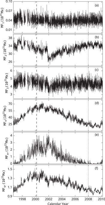
Figure 1. Daily total flux of the magnetic elements in the solar photosphere at the four flux ranges from 1996 September to 2010 February: (a) (1.5–2.9) × 1018 Mx, (b) (2.9–32.0) × 1018 Mx, (c) (3.20–4.27) × 1019 Mx, and (d) (4.27–38.01) × 1019 Mx, as well as the daily total magnetic flux of active regions (e) and quiet regions (f). The vertical thick gray dashed (dotted) line indicates the time of solar maximum (minimum). Note that the units of the vertical coordinates are different. The data were extracted from daily 5-minute-averaged magnetograms of the MDI/SOHO, which was done by Jin et al. (2011).
Download figure:
Standard image High-resolution imageTable 1. Results of Sinusoidal Function Fittings for the Four Types of Magnetic Flux Data
| Data set | Flux Range | T | A | φ | C |
|---|---|---|---|---|---|
| (Mx) | (days) | (Mx) | (radians) | (Mx) | |
| MF1 | (1.5–2.9) × 1018 | ... | ... | ... | ... |
| MF2 | (2.9–32.0) × 1018 | 26.20 | −0.287 ± 0.023 | 0.568 ± 0.079 | −0.072 ± 0.015 |
| MF3 | (3.20–4.27) × 1019 | ... | ... | ... | ... |
| MF4 | (4.27–38.01) × 1019 | 26.23 | 0.363 ± 0.022 | 1.442 ± 0.062 | −0.133 ± 0.048 |
| MFar | Active region | 26.66 | 0.343 ± 0.022 | 1.659 ± 0.065 | −0.003 ± 0.005 |
| MFqr | Quiet region | 26.24 | 0.287 ± 0.023 | 1.169 ± 0.078 | −0.002 ± 0.001 |
Note. T is the period obtained by the Lomb–Scargle method in Section 3.1. A is the amplitude, φ the initial phase, and C a constant. Neither MF1 nor MF3 have any significant rotational periods, thus they are not fitted.
Download table as: ASCIITypeset image
3. METHODS AND ANALYSES
3.1. Lomb–Scargle Periodogram
The time interval of the magnetic flux data spans from 1996 September 1 to 2010 February 28, i.e., 4929 days in all. However, on 1139 days there are no records, which amounts to 23.1%. There are many statistical methods to determine periods in a time series, but these methods are mostly only applicable to continuous time series. In the situation here, considering that missing records take up a relatively large percentage, interpolating the time series to make them continuous is inappropriate since it will introduce high noise. It is therefore reasonable to consider the data sets as unevenly spaced data. Therefore, in order to investigate the rotational behavior of the magnetic flux data here, we employ the Lomb–Scargle method. The Lomb–Scargle periodogram (LSP) is particularly suitable for detecting periodic components in unevenly sampled time series with considerable percentage of missing values, and it restricts all calculations to the actually observed or existing values. The LSP was originally proposed by Lomb (1976), based partly on earlier works of Barning (1963) and Vaníček (1971), and it was further extended by Scargle (1982). Zechmeister & Kürster (2009) developed an analytic solution for the generalization, and also discussed the normalizations and the calculation of the false-alarm probability, which has some similarities to the SigSpec method of Reegen (2007). Vio et al. (2010) presented a new general formalism with matrix algebra. The algorithm of LSP is briefly introduced below.
We assume a time series X with n data points  ,
,  . Then, the normalized Lomb–Scargle spectral power P as a function of the angular frequency ω is defined by
where wi is the normalized weight, and they should be obtained from the data errors. The constant τ is a kind of offset that makes P(ω) completely independent of shifting all the tis by any constant, and it is defined by the relation
Since the properties of the noise level in the magnetic flux data are unknown, the normalization method used in Scargle (1982) or Horne & Baliunas (1986) is unsuitable. Instead, we adopt the method suggested by Cumming et al. (1999). The significance level of any peak in the plot of power versus frequency, i.e., the false-alarm probability (FAP), is determined by

The variable m is the number of probed independent frequencies (or periods).  indicates the probability that the normalized power can exceed a given value.
This method is used by various investigators for period detections, but not necessarily with the same methods of power normalization and FAP determination (e.g., Zechmeister & Kürster 2009; Chowdhury et al. 2013; Qu & Xie 2013).
The LSPs that display the normalized power versus periods for the six categories of magnetic flux data sets are shown in Figure 2. The range of the examined periods is 2–100 days, and the resolution is 0.01 day. As illustrated in the figure, LSPs of MF2 (panel b), MF4 (panel d), MFar (panel e), and MFqr (panel f) exhibit periods approximate to the solar rotation cycle in the considered period range, and these are the only significant periods. The precise values of the periods are listed in the third column of Table 1. The first three periods lie above the 0.01% significance level, while the period in panel (f) lies below the 0.01% significance level, but above the 0.02% significance level. The LSP of MF3 in panel (c) seems to have a peak similar to the above four panels, but it is not significant; neither does MF1 (panel a) show a significant period.
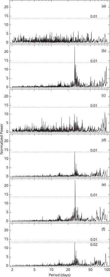
Figure 2. Lomb–Scargle periodograms of the six flux data categories, i.e., four ranges of magnetic flux, plus the flux of active regions and quiet regions. The x-axis indicates the examined periods, and the y-axis shows the normalized power corresponding to each period. The horizontal dotted lines indicate the 0.01% significance level. The 0.02% significance level is also shown in panel (f).
Download figure:
Standard image High-resolution imageIt is indicated in Table 1 that the rotational periods of MF2, MF4, and MFqr are very similar (note that flux of MF2 and MF4 are included in the flux of the quiet regions, MFqr), while that of MFar is higher. Since the longer period corresponds to the lower frequency, it means that active regions rotate more slowly than quiet regions or regions with a weaker magnetic field. This is further discussed in the last section.
3.2. Sinusoidal Function Fitting
Assuming that the rotational periods of four out of the six flux data categories are obtained, we fit each of the four data categories with a sinusoidal function to investigate their phase differences,
For each of the fittings, A is the amplitude, T the period that we obtained in Section 3.1, φ the initial phase, and C a constant. Here, we used a nonlinear least-squares fitting. We are interested in the initial phase φ.
Figure 1 clearly shows intra-cycle related long-term trends superimposed on short-term fluctuations. Therefore, the data sets need to be detrended so as to eliminate the effect of long-term variations. We detrend the data by subtracting their corresponding 26-day filtered lines, which removes signals with periods longer than about 26 days and retains only short-term fluctuations. Furthermore, the data sets are centered and normalized by subtracting their mean values and by dividing them by their standard deviations. The fitting results are show in the last three columns of Table 1.
As can be seen by comparison, the differences among the initial phases of the other three data sets ( ,
,  ,
,  ) with that of active region (
 ) are −1.09, −0.22, and −0.49 radians, respectively. Since the length of one T (∼26 days) corresponds to
  radians, one day corresponds to ∼0.24 radians. Therefore, the phase differences are corresponding to −5, −1, and −2 days, respectively. This shows that at the rotational timescale, MFar leads MF2, MF4, and MFqr by 5, 1, and 2 days, respectively.
If the data sets are not centered and normalized, then the fitting results are different in As and Cs; however, the values of the initial phase  are the same when they are rounded to three digits. If the number of days for detrending is different (for example, from one T to several Ts), then the values of φs are also different, but the differences between
  ,
,  ,
,  , and
, and  are very approximate to the results mentioned above.
3.3. Cross-correlation Analyses
In order to further investigate the phase relations between the magnetic flux of different ranges, we use the cross-correlation analysis. In this study, the sample Pearson correlation coefficient is used. As an example, we assume two data sets with an equal length, { } and {
 } (assuming that the index of the first element of an array is 1 and the last index is n), then their lagged cross-correlation coefficient rxy as a function of the lag k can be written as
where xi indicates the ith element of data set { }. In the calculation, missing records are excluded. For instance, if xa is missing, then in the process of calculating rxy(k) (assuming
  ), the pair of data (xa,
  ) are excluded in the calculation of both the numerator and the denominator of the lower formula. Therefore, the calculation of the cross-correlation coefficients is restricted to the available values, without imposing any interpolations. The cross-correlation method is widely used in determining the mutual correlation and phase relation between two time series (e.g., Edelson & Krolik 1988; Peterson et al. 1998; Chu et al. 2010; Xiang & Kong 2015).
Using this method, we present the cross-correlogram between MF2 and MFar in Figure 3. As shown in the upper panel, when MF2 is lagged by 350 days, which is approximately one year, their correlation coefficient (cc) peaks negatively. Noticeably, in this case, since they are negatively correlated, the meaning is that the maximum of MFar occurs around 350 days ahead of the minimum of MF2. For example, Saito & Tanaka (1960) found a similar phase relation between the abundance of polar faculae and sunspot numbers. The bottom panel shows that when MF2 is lagged by 5 days, their cc peaks negatively, which agrees with the results obtained in Section 3.2. This means that at the timescale of the solar activity cycle, MFar leads MF2 by around one year in time phase, and at the timescale of the solar rotation period, the former leads the latter by 5 days.
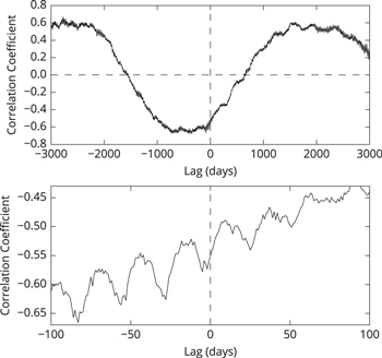
Figure 3. Cross-correlograms between flux data MF2 and that of active regions MFar. The bottom panel is an enlargement of the central part of the upper panel to show their correlation at the timescale of the solar rotation period. The vertical dashed lines indicate 0 day lag, and the horizontal dashed line in the upper panel indicates a correlation coefficient of 0.0.
Download figure:
Standard image High-resolution imageThe ccs for MF4 and MFar are displayed in Figure 4. The upper panel shows that their cc peaks positively when the former is lagged by 82 days (∼3 rotation periods). The bottom panel shows that when MF2 is lagged by 1 days, their cc peaks, which also agrees with the result obtained in Section 3.2. This reveals that at the timescale of the solar activity cycle, MFar leads MF2 by around 3 rotation periods, while at the timescale of the solar rotation period, the former leads the latter by 1 day.

Figure 4. The same as Figure 3, but between the magnetic flux in the range MF4 and the flux of active regions MFar.
Download figure:
Standard image High-resolution imageThe cross-correlogram between MFqr and MFar is displayed in Figure 5. It indicates that at the timescale of the solar activity cycle, MFqr is in phase with MFar, although there is a dip around 0 lag; at the timescale of the solar rotation period, they are anticorrelated. This relation between MFqr and MFar does not agree with the findings in Section 3.2.
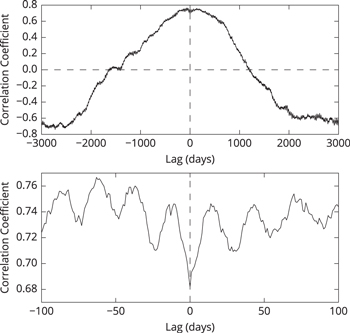
Figure 5. The same as Figure 3, but between the magnetic flux of quiet regions MFqr and the flux of active regions MFar.
Download figure:
Standard image High-resolution imageAs shown in Figure 2 in Jin et al. (2011), MFar and MFqr vary concordantly with the sunspot cycle, although the variation amplitude of MFqr is much smaller. MF2 and MF4 exhibit anticorrelation and incorrelation with the sunspot numbers, respectively. These results are confirmed in the upper panels of Figures 3–5. Furthermore, their phase relations are investigated and illustrated more concretely here.
The three cross-correlograms also exhibit two similarities: (1) At long timescales (see the upper panels of the three figures), the correlation functions indicate curves of sinusoidal waves with a cycle of around 11 years, which is because the four magnetic fluxes are all modulated by the ∼11-year solar activity cycle; (2) at the timescale of the solar rotational period (see the bottom panels of the three figures), the correlation functions fluctuate with a period of around 26 days. This is obviously due to their rotational periodicities.
4. CONCLUSION AND DISCUSSIONS
Magnetic elements are extracted by Jin et al. (2011) from daily magnetograms of the MDI/SOHO, and the magnetic flux in the solar photosphere is classified into four flux ranges together with the total flux of active regions and quiet regions (these six categories of magnetic flux data are referred to as MF1∼4, MFar and MFqr, as shown in the first and second columns in Table 1). The time interval of the data is from 1996 September 1 to 2010 February 28, which includes the whole solar cycle 23. For the first time, the rotational periodicity and phase difference of the magnetic flux at specific flux ranges are examined. The main results found in this research are listed and discussed below.
- (i)Lomb–Scargle periodograms exhibit that MF2, MF4, MFar, and MFqr show rotation periods, which are 26.20, 26.23, 26.66, and 26.24 days, respectively. The period resolution in the analyses is 0.01 day. The rotation periods of MF2, MF4, and MFqr are quite similar, while that of MFar is longer. MF1 and MF3 do not indicate any significant rotation periods. In order to verify the resulting values of the periods, we analyzed the data with another period determination technique named phase dispersion minimization (PDM, Stellingwerf 1978), which is also widely used for astronomical and other types of non-sinusoidal and irregularly spaced data analyses. The differences of the resulting periods between PDM and LSP are within 0.02 days (26.20, 26.23, 26.68, and 26.23 days for MF2, MF4, MFar, and MFqr, respectively).The rotation period of MFar is longer than the other three fluxes, which means that from a global perspective, magnetic fields ain active regions rotate more slowly than quiet regions or weaker magnetic fields.The rotation rate of the solar interior at a different depth from the core to the subsurface shear layer can be determined by helioseismic inferences, and great insight has been obtained in the past four decades (see Howe 2009 and references therein). Studies of the surface rotation reveal that the solar differential rotation shows a cyclic variation pattern that can be described as a torsional oscillation: the rotation rates in certain latitudinal bands speed up or slow down periodically during the solar cycle, while the rates remain steady in other bands (Howard & Labonte 1980). Helioseismic results indicate that the surface torsional oscillation pattern extends throughout the convection zone (e.g., Howe et al. 2000; Vorontsov 2002). In the studies of solar surface rotation, the tracer method is one of the earliest and yet long-standing methods in addition to spectroscopic and helioseismology methods. Various useful solar features are used as tracers to measure the rotation of the Sun, such as sunspots, faculae, plages, supergranules, giant cells, and coronal holes. Almost all of them have a magnetic nature. It is commonly found that magnetic features rotate faster than their surrounding surface plasma (Beck 2000). By making inferences about the internal rotation speed of the Sun through measuring p-mode frequencies, the helioseismology method shows that the maximum rotation rate is at a depth of 0.93
 in the convection zone (Thompson et al. 1996; Schou et al. 1998). It is thus speculated that the anchor foot of the magnetic features penetrates the solar photosphere into the convection zone, and they consequently rotate faster than the solar surface (Beck 2000). Meunier (1999) used the first two years of data of MDI/SOHO 96-minute cadence magnetograms to detect the motion of the solar surface through the cross-correlation analysis, and also found that active regions rotate slightly faster.However, studies of the rotation rate of sunspots of different sizess and age reveal that recurrent sunspots rotate more slowly than young sunspots, and sunspot groups rotate more slowly than sunspots; in other words, the larger the sunspots, or the stronger the magnetic field of the active regions, the slower the rotation rate (see Figures 5 and 8 in Howard 1984; Snodgrass 1983; Beck 2000). The equatorial rotation rate at high activity is found to be lower than the rotation rate at low activity (Meunier 1999). When large sunspots appear on the solar disk at solar maximum time, the rotation rates at various latitudes decrease (see Figure 4 in Li et al. 2013a).Brajša et al. (2006) studied the variation in solar rotation with sunspot groups and found that the rotation velocity is higher than average at the time of solar activity minimum. They inferred that strong magnetic fields repress differential rotation, while when magnetic fields are weaker, a more pronounced differential rotation can be expected. A similar conclusion is also obtained by Zaatri et al. (2009), Wöhl et al. (2010), and Jurdana-Šepić et al. (2011), who studied the solar rotation with bright coronal structures. Li et al. (2013a, 2013b) investigated the solar-cycle-related variation of differential rotation through latitudinally and temporally distributed data of rotation rates derived from synoptic magnetic maps produced by NSO/Kitt Peak and MDI/SOHO (Chu et al. 2010). Their findings confirm that strong magnetic fields repress the differentiation of the solar rotation, while weak magnetic fields seem to reflect the differentiation of rotation rates.These results explain why the rotational signals in the magnetic flux data indicate that MFar rotates more slowly than in weaker magnetic fields (MF2, MF4, and MFqr), and this should be a result of the complex impacts including differential rotation, latitudinal drift of active regions, and the repression of strong magnetic fields. Xiang et al. (2014) used indirect indices and found that the rotation cycle of MWSI is longger than that of MPSI (the former index is a proxy of the strong magnetic field, and the latter a proxy of the weak magnetic field), which is in accordance with our result.
 - (ii)At the timescale of a solar rotation period, sinusoidal function fittings indicate that MFar leads MF2 and MF4 by 5 and 1 days, respectively, which is further confirmed by cross-correlation analyses. However, the phase difference between MFqr and MFar obtained from the cross-correlogram is not consistent with the difference obtained from the fitting. The reason is probably that φ obtained from the fitting does not contain information of the solar activity cycle, while the cross-correlation analysis is modulated by the solar activity cycle. In addition, phases found through fitting correspond to different frequencies or periods, while the cross-correlation analysis does not take the difference of frequencies into consideration.The lags between MF2, MF4, and MFar are speculated to be associated with the evolution of active regions and the surface magnetic field. The magnetic signals recorded by magnetograms are dominated by a dynamo that is located in or below the solar convection zone (Charbonneau 2010). Some of the toroidal fields rise from there and reach the solar surface as magnetic flux tubes. These are affected by convection and rotation, and then evolve and decay in a complex way (Fan 2009; Jiang et al. 2014). It is conjectured here that active regions evolve and decay into magnetic elements at range MF4 after 1 day and into magnetic elements at range MF2 in 5 days on average, which agrees well with the lifetime of the majority of sunspots (Petrovay & Driel-Gesztelyi 1997; Solanki 2003).
- (iii)At the timescale of the solar cycle, MF2 and MFar are negatively correlated, and the former lags the latter by 350 days (around one year). MF4 and MFar are positively correlated, and the former lags the latter by 82 days (around 3 solar rotation periods). The reason for this phase relation is not yet clear. Additionally, MFqr and MFar are also positively correlated.

It is speculated that the magnetic elements contributing to MF2 mainly come from higher latitudes. The phase relation between solar activities at high and low latitude has been extensively studied, and it is basically confirmed that they are not in phase (Li et al. 2006a). For example, early results by Saito & Tanaka (1960) show an evident anticorrelation between the abundance of polar faculae and sunspot activity, and the maximum of the former occurs 1 year ahead of the minimum of the latter. Li et al. (2002b) confirmed that the maximum years of polar faculae abundance occurred during the minimum years of sunspot numbers. Li et al. (2002a) examined the phase relation between high- and low-latitude activities of solar active prominences, and discovered that the activity of solar active prominences peaks earlier in higher latitudes. The cycle of solar active prominences in high latitudes leads both the sunspot cycle and the corresponding cycle of solar active prominences in low latitudes by 4 years. Sunspot numbers are commonly used as a proxy of low-latitude magnetic field activities (Li et al. 2006b); MFar is obviously a more direct measurement. The phase relation between MF2 and MFar is very similar to that between high- and low-latitude solar activities. Note that the magnetic fluxes used in this study are extracted from magnetograms up to 60°.
Another possibility is that MF2 emerges from the subsurface shear layer (also named leptocline), which is a strongly variable layer located at around a depth of  . The acoustic radius of this layer obtained through helioseismology is in antiphase with the solar activity, while that of the deeper layers of the Sun, between 0.975 and
  , changes in phase with the 11-year solar cycle (Lefebvre & Kosovichev 2005). Many phenomena take place in the subsurface shear layer, such as an oscillation phase of the seismic radius and changes in the turbulent pressure and opacities, and it probably is the seat of in situ magnetic fields (Rozelot et al. 2009).
The phase relation between MFar and MF4 suggests that the magnetic flux in in situ magnetic fields may partly come from that of the former, i.e., the weak magnetic field in MF4 partly comes from the evolution of active regions. Based on studies of MWSI and MPSI, Xiang et al. (2014) found a similar result. However, our research shows that the weak magnetic flux in MF4 lags MFar by around three rotation periods, instead of around one rotation period as in Xiang et al. (2014). The reason probably is that the magnetic flux data sets used here are direct measurements, and the flux ranges are more specific.
By performing simulations with different parameters of Reynolds and dynamo numbers, Karak & Brandenburg (2016) explored the solar cycle dependence of small-scale magnetic fields. They concluded that MF4 might come form the shredding and tangling of the large-scale magnetic field generated by the global dynamo alone, while the behavior of MF2 requires a small-scale dynamo that is generated locally in the solar convection zone (in addition to the large-scale magnetic field that is generated by the global dynamo). However, if MF2 comes from higher latitudes or emerges from the subsurface shear layer, then the reason for the necessity of the small-scale dynamo is not entirely convincing.
Li et al. (2013a) studied the solar-cycle-related differential rotation in solar cycles 21–23 together with the north–south asymmetry, and found that the northern hemisphere rotates slightly faster than the southern hemisphere; the degree of asymmetry is generally higher during solar maximum. However, because the data set length we used is limited, we are unable to inspect whether the result is different from cycle to cycle, or if there is a north–south asymmetry. Moreover, if information about the latitudes of magnetic elements were available, it would be possible to study the differential rotation of the surface magnetic field with data at various flux ranges.
The authors would like to express their deep thanks to C. L. Jin for providing the data. We thank Prof. Shadia R. Habbal and the anonymous referee for insightful comments and rigorous doubts and suggestions that helped improve the manuscript. This work made use of open-source scientific tools including Numpy (Walt et al. 2011), Scipy (Jones et al. 2001), Matplotlib (Hunter 2007), IPython (Perez & Granger 2007), astroML (VanderPlas et al. 2012), PyAstronomy5 , and Jupyter.6 This work is supported by the National Natural Science Foundation of China (11573065, 11633008, 11273057, and 11673061), the Specialized Research Fund for State Key Laboratories, the Chinese Academy of Sciences, and the Applied Basic Research Foundation of Yunnan Province, China (Grant Nos. 2014FB190).