


Abstract
We present a study of 323 photometrically variable young stellar objects that are likely members of the North America and Pelican nebulae star-forming region. To do so, we utilize over two years of data in the g and r photometric bands from the Zwicky Transient Facility. We first investigate periodic variability, finding 46 objects (∼15% of the sample) with significant periods that phase well and can be attributed to stellar rotation. We then use the quasiperiodicity (Q) and flux asymmetry (M) variability metrics to assign morphological classifications to the remaining aperiodic light curves. Another ∼39% of the variable star sample beyond the periodic (low Q) sources are also flux-symmetric, but with a quasiperiodic (moderate Q) or stochastic (high Q) nature. Concerning flux-asymmetric sources, our analysis reveals ∼14% bursters (high negative M) and ∼29% dippers (high positive M). We also investigate the relationship between variability slopes in the g versus g − r color–magnitude diagram, and the light-curve morphological classes. Burster-type objects have shallow slopes, while dipper-type variables tend to have higher slopes that are consistent with extinction-driven variability. Our work is one of the earliest applications of the Q and M metrics to ground-based data. We therefore contrast the Q values of high-cadence and high-precision space-based data, for which these metrics were designed, with Q determinations resulting from degraded space-based light curves that have the cadence and photometric precision characteristic of ground-based data.
Export citation and abstract BibTeX RIS

Original content from this work may be used under the terms of the Creative Commons Attribution 4.0 licence. Any further distribution of this work must maintain attribution to the author(s) and the title of the work, journal citation and DOI.
1. Introduction
The Zwicky Transient Facility (ZTF; Kulkarni 2018) has been used prolifically in contemporary transient detection and characterization efforts. Astrophysical transients observed and/or discovered by ZTF include: tidal disruption events (e.g., van Velzen et al. 2021), candidate electromagnetic counterparts to gravitational wave events (e.g., Graham et al. 2020), type Ia supernovae (e.g., Yao et al. 2019; Bulla et al. 2020; Miller et al. 2020), dwarf novae (e.g., Soraisam et al. 2021), cataclysmic variables (e.g., Szkody et al. 2020), AM CvN systems (van Roestel et al. 2021a), general stellar variables (e.g., Roulston et al. 2021; van Roestel et al. 2021b), active galactic nuclei (e.g., Frederick et al. 2019; Ward et al. 2021), and solar system bodies such as comets and asteroids (e.g., Ye et al. 2020b, 2020a).
While photometric variability has long been known as a ubiquitous characteristic of young stellar objects (Joy 1945), no study to date has utilized the ZTF for investigating the variability behavior generally in young stars, based on a significantly large sample. ZTF data have, however, contributed to investigations of young stellar objects (YSOs) in several studies focused on individual sources (e.g., Dahm & Hillenbrand 2020; Hodapp et al. 2020; Hillenbrand et al. 2022). The plethora of multiyear, nearly nightly cadence, and multicolor ZTF observations is ideally suited for studying the variability of optically visible YSOs.
Our study targets a sample of YSOs in the vicinity of the North America and Pelican (hereafter NAP) nebulae (Reipurth & Schneider 2008). Initial interest in this region as a laboratory for studying the evolution and variability of YSOs was piqued after Herbig (1958) identified and characterized numerous YSOs based on Hα emission lines. More recently, Guieu et al. (2009) and Rebull et al. (2011) identified more than 2000 candidate YSOs in the region based on infrared excess emission using data from Spitzer (Werner et al. 2004) and the Two Micron All Sky Survey (2MASS; Skrutskie et al. 2006). Focusing on the L935 dark cloud region, Armond et al. 2011 identified new Hα emitters and Herbig–Haro flows, and Damiani et al. (2017) studied X-ray emitters. These catalogs have been of interest in recent years for other studies investigating various aspects of the young stars in the region, including kinematics (Kuhn et al. 2020) and Hertzsprung–Russell (H-R) diagrams (Fang et al. 2020).
Considering previous variability studies, Findeisen et al. (2013) identified 43 large-amplitude aperiodic variables with distinct bursting or fading behavior, which is believed to be driven by variable accretion and extinction processes, respectively (e.g., Herbst et al. 2002; Cody & Hillenbrand 2018). The results of long-term photometric monitoring observations of the region have been reported by Poljančić et al. (2014), Ibryamov et al. (2015), and Ibryamov et al. (2018), providing detailed analyses of small samples of stars based on decades of multicolor data from numerous observatories. Bhardwaj et al. (2019) found 56 periodic variables in the Pelican Nebula region, visually classifying an additional 11 variables as nonperiodic while Froebrich et al. (2021) identified 59 periodic variables, many of which overlap with the Bhardwaj et al. (2019) sample.
In this paper, we utilize the flux asymmetry and quasiperiodicity metrics of Cody et al. (2014) to quantitatively describe variability classes of YSOs in the region, greatly expanding upon the results of previous variability studies. In doing so, we present the largest single sample of YSOs classified by the flux asymmetry and quasiperiodicity metrics to date. We connect the light-curve classifications with analysis of color–magnitude variability trends, which helps to provide a more comprehensive understanding of the nature of the variability.
The remainder of this paper is structured as follows. We describe our stellar sample in Section 2 and the observations used as well as data selection and handling in Section 3. The identification of variability and the search for periodicities are discussed in Section 4. In Section 5 we present our light-curve classification and color–magnitude results. In Section 6 we consider relationships of the variability patterns to the presence of circumstellar disks. We discuss our results in the context of other recent studies in Section 7, and summarize our findings in Section 8. Several appendices present: the full light-curve set, the results of testing performance of one of the variability metrics (quasiperiodicity) with data cadence and precision, and our findings on the periodograms for two particularly interesting sources.
2. Sample Selection
Our sample consists of YSOs in the NAP nebulae that have been promoted as members based on kinematic, spectroscopic, and H-R diagram selection criteria.
The starting list for this investigation was created by crossmatching all 580 objects from Table 4 in Fang et al. (2020) with all 395 objects from Table 2 in Kuhn et al. (2020) using a match radius of 0 5. The combined sample of 696 sources includes every source in either of those tables, with 301 uniquely from Fang et al. (2020) and 116 uniquely from Kuhn et al. (2020).
In Kuhn et al. (2020), membership was assessed using Gaia kinematics for all candidate members of the NAP nebulae complex previously suggested as such in the literature. In Fang et al. (2020), membership for stars with optical spectroscopic data was assessed from a combination of indicators. These included stellar activity manifest through X-rays and accretion-related optical emission lines, infrared excess indicative of circumstellar dust, lithium absorption, and criteria on parallax and proper motions.
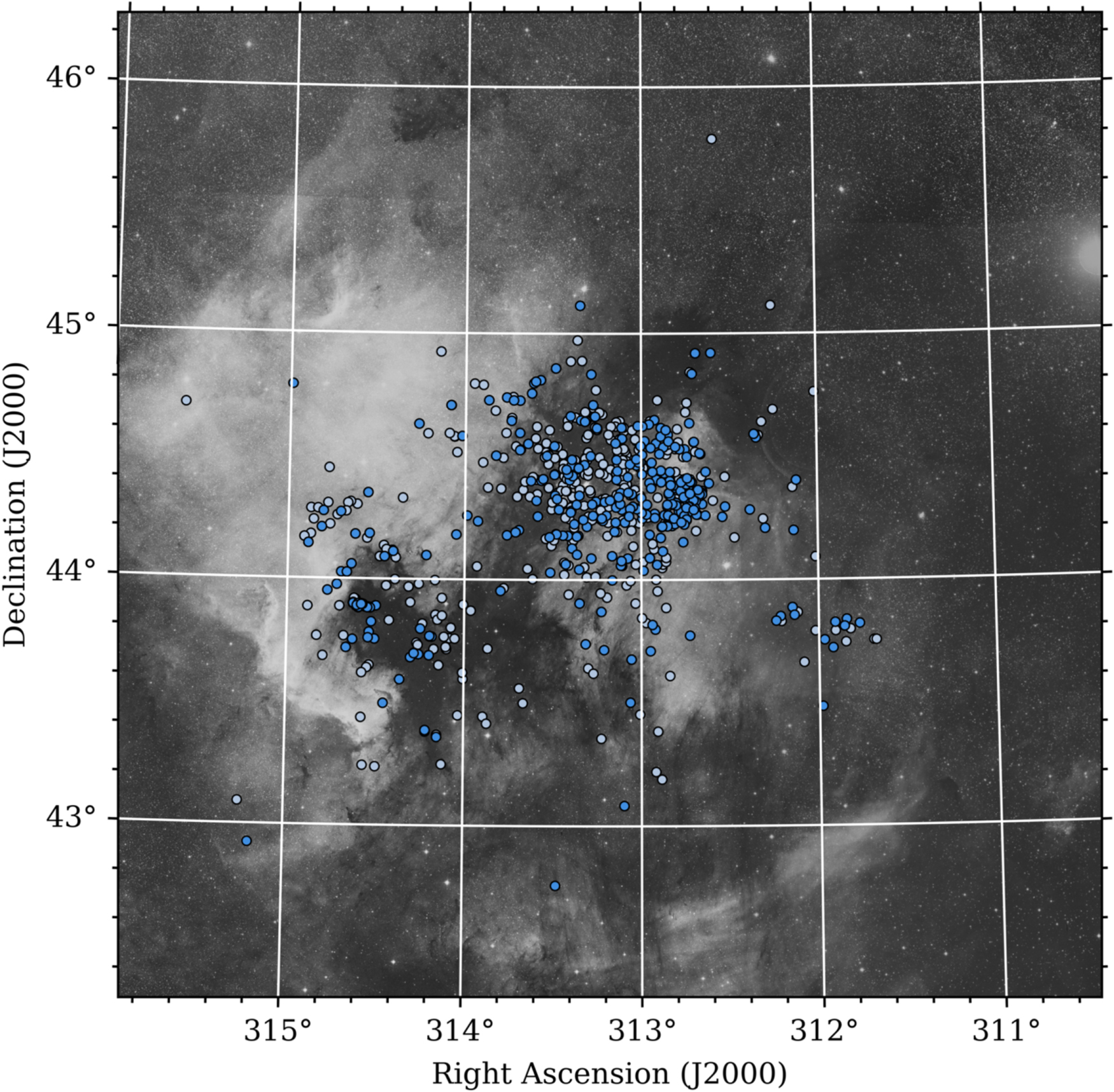
Figure 1 shows the spatial distribution of the initial sample as well as the reduced, final sample discussed below.

Figure 1. Full sample of selected likely members of the North America (left) and Pelican (center) nebulae star-forming complex plotted over a DSS2-R red photographic image of the region. Our final sample of 323 variable sources from the ZTF is in darker blue, with the remaining likely member sources that do not meet all of the applied ZTF photometric cuts represented in lighter blue.
Download figure:
Standard image High-resolution image3. ZTF Photometry
The ZTF (Bellm et al. 2019) employs the 48 inch Schmidt telescope at Palomar Observatory and possesses a camera with a 47 deg2 field of view. It efficiently surveys the northern sky, cataloging more than a billion objects since first light in 2018 (Masci et al. 2019). The ZTF serves as the current standard for rapid cadence, ground-based photometric surveys as well as a test bed for techniques to be used in upcoming next generation surveys such as the Large-aperture Synoptic Survey Telescope (Graham et al. 2019).
In this paper, we analyze data from the fourth public ZTF data release (ZTF DR4), which corresponds to more than two years of data taken in the NAP field between 2018 March 28 and 2020 June 6 (58205 ≤ MJD ≤ 59028). We focus our analysis on the ZTF g-band (λeff = 4722 Å) and r-band (λeff = 6340 Å) data, as the long-term i-band survey mainly covers high-galactic-latitude fields. We refer the reader to Bellm et al. (2019) and Masci et al. (2019) for in depth descriptions of the ZTF observing and image processing systems. The photometry is calibrated to Panoramic Survey Telescope and Rapid Response System (PanSTARRS) photometry (with g having λeff = 4811 Å and r having λeff = 6156 Å) and reported in AB magnitudes.
Two objects were removed from the sample (2MASS J20505838+4414444 near FHK 47 = V1597 Cyg A, and Gaia DR2 2163143481019730688 near FHK 67) because they are the fainter members of close pairs, and the photometry is spatially unresolved in the ZTF. We additionally note that while 2MASS J20593270+4408353 and FHK 485 are spatially resolved in ZTF images, their photometry and hence light curves appear cross-contaminated.
The median cadence of the ZTF light curves in the NAP region is ∼1 day. The observations were generally taken nightly, apart from seasonal gaps of ∼30 days plus additional short gaps due to adverse weather. We ignore observations affected by clouds and/or the moon (these observations have catflag = 32768). We also ignore the observations between 58448 and 58456 MJD as these epochs encompass the ZTF high-cadence experiments (Kupfer et al. 2021), which have some noticeably poor photometry in the NAP region due to bad weather that adversely impacts period searches and color–magnitude analysis.
For our analysis, we restrict the sample to objects with mean g < 20.8 mag or mean r < 20.6 mag over the entire time series. We further require at least 30 observations in both the g band and r band (after the application of a 5σ clip of potential outliers from the median magnitude of the light curve). A summary of the cuts applied to our initial sample and its reduction to our final sample for light-curve analysis is provided in Table 1. Figure 2 shows the photometric precision of the r-band observations as a function of median r magnitude for objects in our final sample.

Figure 2. Mean 1σ photometric uncertainty as a function of mean r magnitude, calculated from the ZTF DR4 data products. Objects in our final variable star sample are shown in darker blue, and those not meeting all photometric cuts in lighter blue. The outlier at r ≈ 18 and σr ≈ 0.06 is FHK 96, a source that undergoes an abrupt dimming event of >4.5 mag approximately halfway through the observing window.
Download figure:
Standard image High-resolution imageTable 1. Remaining Sample Size following Application of Selection Criteria
| Criterion | # in Sample |
|---|---|
| Initial sample of likely NAP members | 696 |
| Spatially resolved in the ZTF | 694 |
| Brightness g < 20.8 or r < 20.6 mag | 410 |
| Epochs > 30 for both g and r | 392 |
| Variability level ν > 15 th percentile | 323 |
Download table as: ASCIITypeset image
4. Photometry Analysis
The r-band light curves, g versus g − r color–magnitude trends, and periodogram results are illustrated for a set of representative sources in Appendix A; the full sample is available in an online figure set.
The results of our ZTF light-curve analysis as described below appear in Table 2. Source identifiers were adopted in the order: LkHα numbers from Herbig (1958), V* identifiers from the General Catalog of Variable Stars (Samus et al. 2017; see also Samus et al. 2021 for a history), FHK identifiers from Fang et al. (2020), then catalog identifiers from 2MASS Cutri et al. (2003) and finally Gaia DR2 Gaia Collaboration et al. (2018).
Table 2. Properties of Variable Stars in our NAP Sample
| Identifier | R.A. | Decl.. | Timescale | Q | M | ν | 〈r〉 | Primary | Secondary | CMD |
|---|---|---|---|---|---|---|---|---|---|---|
| or Period | Var. Class | Var. Class | Angle | |||||||
| (deg) | (deg) | (day) | (mag) | (deg) | ||||||
| V752 Cyg | 314.63997 | 44.05985 | 6.652 | 0.93 | −0.05 | 0.0824 | 16.06 | S | ⋯ | 67.6 |
| V1716 Cyg | 314.52548 | 43.88363 | 4.140 | 0.77 | −0.49 | 0.0179 | 16.54 | B | P | 63.2 |
| V1701 Cyg | 312.75373 | 44.53047 | 6.937 | 0.92 | 0.81 | 0.0840 | 15.96 | APD | ⋯ | 80.5 |
| V1597 Cyg | 312.74346 | 44.24561 | 3.422 | 0.86 | −0.12 | 0.0087 | 15.05 | QPS | ⋯ | 48.3 |
| V1492 Cyg | 312.77375 | 44.27562 | 10.48 | 0.88 | 0.39 | 0.0549 | 14.88 | QPD | ⋯ | 74.9 |
| V1490 Cyg | 312.72325 | 44.35025 | 31.17 | 0.67 | 0.71 | 0.0571 | 14.96 | QPD | ⋯ | 81.9 |
| LkHA 191 | 314.77429 | 43.95086 | ⋯ | 0.90 | −0.89 | 0.0113 | 12.44 | B | ⋯ | 7.5 |
| LkHA 189 | 314.60004 | 43.89850 | 2.449 | 0.73 | 0.34 | 0.0118 | 15.57 | QPS | L | 65.3 |
| LkHA 188 | 314.59921 | 43.88648 | 1.011 | 0.78 | 0.84 | 0.0406 | 13.16 | QPD | ⋯ | 74.3 |
| LkHA 187 | 314.58975 | 43.89581 | 2.873 | 0.82 | 0.03 | 0.0095 | 16.32 | QPS | ⋯ | 59.6 |
Notes. A full, machine-readable, version of this table is available electronically. Timescale or Period = Lomb–Scargle periodogram peak that is identified with a period when the Primary Var. Class column is "P"; otherwise interpreted as a variability timescale and not a strict period.
Q = light-curve quasiperiodicity metric defined in Equation (2).
M = light-curve asymmetry metric defined in Equation (3).
ν = variability metric defined in Equation (1).
〈r〉 = mean magnitude over ZTF time series.
Primary Variability Class = dominant behavior in the light curve, classified as one of: P = strictly periodic; MP = multiperiodic; QPS = quasiperiodic, symmetric; QPD = quasiperiodic, dipping; APD = aperiodic, dipping; S = stochastic or aperiodic, symmetric behavior.
Secondary Variability Class = additional, subordinate behavior exhibited in the light curve, using the same classification scheme as above.
CMD Angle = fitted slope to the g vs. g − r color–magnitude diagram, reported only when the error is < 10°.
Only a portion of this table is shown here to demonstrate its form and content. A machine-readable version of the full table is available.
Download table as: DataTypeset image
Photometric variability amplitude, and timescale or period (as appropriate) are discussed in this section. Light-curve asymmetry and waveform repeatability are presented in the next section.
4.1. Variability Search
We utilize the normalized peak-to-peak variability metric

featured in Sokolovsky et al. (2017) to quantify variability amplitude for objects in our YSO sample. In this formula, mi represents a magnitude measurement and σi represents the corresponding measurement error, with the minimum and maximum determined from the full light curve. We eliminated possible outliers with the application of a 5σ clip to all light curves, before calculating ν; this is necessary for the metric to be considered a sensitive variability indicator. For each r-band light curve in our sample that meets the measures described in Section 3, we calculate ν. We note that ν correlates well with standard deviation, with values that are about a factor of 6 smaller.
Our final sample for variability analysis includes objects with ν greater than the 15th percentile of ν as a function of magnitude. Although not a rigorously justified cutoff, this criterion ensures that we are studying the fractionally larger amplitude variables at each brightness level. Figure 3 depicts the selection of sources based on ν, and Table 1 shows the effect of the ν cut on our final sample size.

Figure 3. Normalized peak-to-peak variability metric ν as a function of mean r magnitude for our sample of 392 NAP stars that meet the cuts on magnitude and minimum number of observations. Objects in darker blue above the dashed 15th percentile line are the 323 sources included in our variable star sample, while those not included are in lighter blue.
Download figure:
Standard image High-resolution image4.2. Period Search
We use the Astropy implementation of the Lomb–Scargle periodogram (VanderPlas et al. 2012; VanderPlas & Ivezić 2015) to search for periodic signals in the ∼825 day ZTF data stream. Possible periods between 0.5 and 250 days are considered.
We compute the periodogram for every object in the variable sample, flagging periods between 0.5–0.51, 0.98–1.02, 1.96–2.04, and 26–30 days for further analysis to avoid the most common aliases associated with the solar and sidereal days, as well as the lunar cycle (following Rodriguez et al. 2017; Ansdell et al. 2018). In particular, the window function shows that we have the potential for extremely strong signals at frequencies corresponding to 1.000 and 0.997 day periods. To account for additional potentially aliased periods, we flag periods with half or double multiples that fail at least one of the aforementioned alias checks. We then compute the 90%, 95%, and 99% confidence false alarm probability levels, and consider the period corresponding to the highest power peak greater than the 99% confidence false alarm probability (FAP; < 0.01) to be significant (following Messina et al. 2010). While FAP values may not be as reliable as formal hypothesis tests, they are sufficient for our purpose here, which is to identify potential variability timescales for visual examination and further assessment.
We repeat the above procedure with g-band data for objects lacking a significant period in r. If a significant period is found in g, we return this period for the source.
For each object, the full light curve was phased at the four most significant peaks and visually examined to assess the dispersion across phase. We also marked periods corresponding to beats of the ∼1 day sampling interval to assess the expected Fourier patterns. The periodograms are quite clean in terms of signal-to-noise. In the vast majority of cases, the highest periodogram peak was retained as correct, with recognizable harmonic aliasing and beats having lower power. In some cases, a longer period with a slightly less prominent peak was retained as the most likely true period based on better explanation of the beat patterns, and improved phase dispersion minimization. We call attention to two particularly interesting and nonintuitive examples in Appendix B.
Objects with significant Lomb–Scargle periodogram peaks in either r or g that passed our vetting procedures are reported in Table 2. We have labeled the relevant column as containing both timescales and true periods. In cases where the value of Q (quasiperiodicity metric; see next section) is high, the periodogram peaks are more appropriately thought of as timescales, whereas when Q is low, the light curve is truly periodic in the sense of strictly repeating, with low residual dispersion in the phased light curve. In this latter case, there is also a "P" in the column containing the primary variability classification. A few sources have multiple significant real (nonalias or nonbeat) peaks in the periodogram, and are given "MP" classifications.
The distribution of periods for the sources identified as strictly periodic is shown in the lower panel of Figure 4. There are 46 such stars, constituting ∼15% of the variable sample with reported timescales or periods in Table 2. Their period distribution has a bimodal peak, as well as a skew toward longer periods. Both features are consistent with the populations of fast and slow rotators discussed in previous young star literature, e.g., Gallet & Bouvier (2013).

Figure 4. Distribution of significant Lomb–Scargle periodogram peaks. Top panel shows shows all timescales from Table 2, regardless of light-curve classification. Bottom panel shows only stars labeled as "P" in Table 2, which are those that phase well to their periodogram peaks and likely have their origin in spot pattern modulation due to stellar rotation. As expected, the true stellar rotation periods are concentrated toward the shorter timescales, with values of a few days to a few weeks.
Download figure:
Standard image High-resolution imageFigure 4 also shows, in the upper panel, the full range of variability timescales in the sample. This distribution exhibits a strong peak on the same few week timescales covered by the purely rotationally variable stars in the lower panel. The peak is significantly higher though, indicating a large quasiperiodic and aperiodic population with additional physical processes that are occurring on similar timescales. The timescale distribution is relatively flat out to longer times. The longer variability patterns, from weeks to months, can be seen in the light curves themselves. We emphasize that, even though these timescales were detected and measured using Lomb–Scargle periodogram techniques, they really are approximate timescales for photometric variability, and not true periods. Particularly in cases of high Q values (see below), these timescales are less trustworthy. Other methods for quantifying timescales in aperiodic light curves are discussed in Findeisen et al. (2015).
One particular source with a credible long period or timescale is V1490 Cyg, with a timescale of 31 days. In this case, the phased light curve shows substantially variable depth dips that are more consistent with material orbiting in a disk than with, e.g., a stellar rotation period.
We also performed a Lomb–Scargle period search on the g − r color curves, with colors created from the individual g and r time series as described below in Section 5.2. Few objects were found with significant periodicity in their colors. Among them, FHK 216 and FHK 442 are examples with periodic color variations. While their color curves do not phase particularly well, the color periods are the same as the single-band periods, reported in Table 2. FHK 216 has a color–magnitude slope similar to the reddening vector while FHK 442 is slightly shallower.
5. Light-curve Classification
5.1. Q and M Variability Metrics
Our light-curve classification scheme follows the methodology of using statistics that quantify quasiperiodicity and flux asymmetry, first developed by Cody et al. (2014) and further refined by Cody & Hillenbrand (2018). Quasiperiodicity, Q, is defined as

where σphot is the measurement uncertainty,  is the variance of the original light curve, and
  is the variance of the residual light curve after the smoothed dominant periodic signal has been subtracted. We take σphot as the mean photometric error for all observations in an object's light curve, multiplied by a factor of 1.25 to account for an initial compression of Q values between 0 and ∼0.6 that we noticed early in our investigation. We attribute this compression to two effects: (1) the likely underestimate of reported photometric errors, and (2) the cadence dependence of the Q metric, which we discuss in Appendix C. For
  , we calculate the residual light curve by adopting a modified version of the periodicity routine described in Section 4.2. The light curve is first phased to the best period. Then, following Bredall et al. (2020), we mitigate for edge effects by concatenating three cycles of the period and convolving with a boxcar window of width 25% of the period, effectively smoothing the light curve by a factor of 4. Finally, we subtract the middle cycle of this model light curve from the folded light curve and compute σresid as the standard deviation of this residual curve. The resulting Q values are expected to fall between 0 (strong periodicity with low residual noise) and 1 (completely stochastic behavior).
Flux asymmetry, M, is defined as

where 〈m10%〉 is the mean of all magnitude measurements in the top and bottom deciles of the light curve, mmed is the median magnitude measurement, and σm is the standard deviation of the light curve (Cody & Hillenbrand 2018). Objects that have M values <0 are predominately brightening, objects with M values >0 are predominantly dimming, and objects with M values near 0 have symmetric light curves. In practice, we follow previous literature and assign M < −0.25 as bursters, M > 0.25 as dippers, and the intermediate M values as relatively symmetric light curves.
We calculate Q and M based on the r-band light-curve data. Figure 5 provides illustrative light curves along the Q and M sequences.

Figure 5. Example ZTF data at low, intermediate, and high values of the asymmetry parameter M (upper panels) and the quasiperiodicity parameter Q (lower panels). Negative values of M indicate flaring or bursting type behavior, while positive values of M signify dipping or fading behavior. Low values of Q indicate more strictly periodic light curves, while high values of Q are characteristic of stochastic light curves.
Download figure:
Standard image High-resolution imageWe then distinguish YSO light curves as populating nine categories, following Cody et al. (2014). We present these classification results in Table 2. In general, the objects are classified based on their Q and M values and then validated by visual examination, but there are cases where we adjust the classification to defer to the human eye for definitive categorization. This is especially prevalent in cases near the morphological boundaries in the Q − M plane.
Periodic variables (P) are defined as objects with significant periods from Section 4.2 that have −0.25 < M < 0.25 and Q < 0.45. We discuss our rationale for using a higher Q boundary for periodic objects than adopted in previous publications (e.g., Cody & Hillenbrand 2018; Bredall et al. 2020), in Section 7.2. The variability of the strictly periodic objects is most commonly interpreted as driven by rotational modulation due to the presence of star spots, and the periods derived are thus considered measures of stellar rotation (e.g., Rebull et al. 2008). Notable in this regard is that the sources with Q < 0.45 populate only the lowest range of the normalized variability amplitude, with ν < 0.02, while sources with higher Q span the full range of ν. Multiperiodic (MP) objects exhibit more than one distinct period, that is not a beat or alias. One common explanation for these is starspot modulation in binary pairs (e.g., Maxted & Hutcheon 2018; Stauffer et al. 2018).
Objects with Q > 0.45 are designated as quasiperiodic or stochastic. For the quasiperiodics, the variability origin is perhaps related to stellar rotation or the star-disk interaction region, but not dominated by the starspot modulation signal, which can become partially obfuscated in cases of a strong inner disk. There are two flavors of quasiperiodic variables, depending on M.
Quasiperiodic symmetric (QPS) variables are defined as having −0.25 < M < 0.25 and 0.45 < Q < 0.87. The variability of these objects is believed to have two possible sources. The first is a combination of purely periodic spot behavior with longer timescale aperiodic changes (e.g., variable accretion), and the second is a single variability process that is unstable from cycle to cycle (Cody et al. 2014).
Quasiperiodic dipper (QPD) variables are categorized based on M > 0.25 and 0.45 < Q < 0.87. The variability of these objects is believed to stem from variable extinction caused by time-variable occultation by circumstellar material (e.g., Alencar et al. 2010; Morales-Calderón et al. 2011; Ansdell et al. 2016). We do not define a quasiperiodic burster category, as distinct from the stochastic bursters, following previous literature in the field.
Burster (B) variables are defined as having M < −0.25, and correspond to objects with erratic but discrete accretion bursts that are generally short-lived (Cody et al. 2017). These bursts are distinct from larger amplitude and longer timescale outbursts from EX Lup and FU Ori type sources, which are more eruptive (Hartmann & Kenyon 1996; Herbig 2008).
Aperiodic dipper variables (APD) are defined as having M > 0.25 and Q > 0.87. These objects experience variable extinction, and it has been proposed by Turner et al. (2014) that their variability stems from inner disk scale-height changes induced by magnetic turbulence.
Stochastic (S) variables are defined as having −0.25 < M < 0.25 and Q > 0.87. They feature nonrepeating variability patterns with relatively symmetric excursions around a median brightness.
Long-timescale (L) objects exhibit variability on timescales ≳ 100 day timescales. They generally have Q > 0.87. Finally, we assign two objects to the unclassifiable (U) category because we were unable to calculate their Q due to  being larger than
  and/or
  .
.
The results of this classification scheme are reported in Table 2 for individual sources. Additionally, all stars in the variable sample are plotted in the Q − M plane in Figure 6, where they are differentiated in color by the assigned (primary) morphological class. The distribution of primary and any secondary variability classes is summarized in Table 3.

Figure 6. Flux asymmetry vs. quasiperiodicity for our sample of variables, color coded by light-curve morphological type as reported in Table 2. The size of each point is proportional to its linearly scaled peak-to-peak variability metric ν. Note that some objects, especially periodic sources with high values of Q, can fall outside of the defined boundaries between the morphological classes in the Q − M plane. However, the Q − M classification is fairly robust with only a minor number of sources deserving adjustment to their numerically assigned classes.
Download figure:
Standard image High-resolution imageTable 3. Distribution of Primary and Secondary Light-curve Morphology Classifications for Objects in our Variable Sample
| Variability Class | Primary % | Secondary % |
|---|---|---|
| Periodic | 14.6 | 0.9 |
| Multiperiodic | 0.6 | 1.9 |
| Quasiperiodic symmetric | 27.6 | 0.3 |
| Quasiperiodic dipper | 19.2 | ⋯ |
| Aperiodic dipper | 9.6 | ⋯ |
| Burster | 13.9 | ⋯ |
| Long timescale | 2.8 | 12.7 |
| Stochastic | 11.5 | ⋯ |
| Unclassifiable | 0.3 | ⋯ |
| Total | 100.1 | 15.8 |
Note. Most sources have a single dominant variability type, but ∼16% of the variable sample merited secondary classifications. Values in individual rows have been rounded.
Download table as: ASCIITypeset image
Objects have secondary classifications in Table 2 when more than one light-curve type is evident in the data. Secondary classifications are typically long-timescale (L), representing objects that exhibit a strong primary behavior such as short timescale periodicity, quasiperiodic behavior, or bursting, along with a pronounced long-term trend such as brightening or dimming, or lasting changes in variability amplitude, etc. We call attention to two objects, V1716 Cyg (FHK 437) and FHK 496 that are designated as periodic in their secondary classification. Both have robust periods that phase very well, but their Q values are high, and the M metric reveals that the full amplitude of the light curve is caused by bursty behavior. As these cases are each somewhat interesting, we detail them here.
For V1716 Cyg, the behavior over most of the light curve is plainly periodic, but for a little over one year of our time series there is superposed continuous bursting at the 1 mag level. Findeisen et al. (2013) also observed bursts in their earlier light curve of this source based on PTF data. The source further distinguishes itself in having—aside from the bursts—a phased light-curve morphology that appears (see Appendix A figure set) similar to a W UMa profile. 5 with V-like troughs, and broad inverted-U-like peaks.
In FHK 496, bursting behavior is ubiquitous throughout the light curve, and causes scatter at the 0.4 mag level above the clear periodic signal, which has lower amplitude.
5.2. Color–Magnitude Analysis
As mentioned above in Section 5.1, there are many different physical mechanisms that can cause photometric variability in young stars. Color time series data can be a helpful tool in distinguishing them. Among others, Carpenter et al. (2001), Günther et al. (2014) and Wolk et al. (2015) showed how near-infrared and mid-infrared multicolor photometry can distinguish extinction-related and accretion-related variability mechanisms. Optical photometry is even more sensitive to these behaviors, due to the steep rise in extinction from the infrared to the optical, and because of the hot nature of the accretion process.
The ZTF g-band and r-band observations are often taken close to one other, within a few hours up to a few days, but they are not simultaneous. Color–magnitude diagrams were thus constructed as follows. First, we partitioned the g-band light curves into segments in which the maximum separation between any two subsequent g observations is less than three days. We adopted this maximum observation separation constraint because linearly interpolating between g observations taken further apart created spurious values in the color–magnitude plane. In practice, within the defined <3.0 day intervals, approximately 20.5% of the g-band observations occur within 0.25 days of the prior g-band observation, 87.0% within 1.25 days, 93.4% within 2.0 days, and 97.5% occur within 2.25 days. For each g-band value that was paired with an r-band observation, we then linearly interpolated between the date bounds of the defined g-band intervals, in order to estimate g − r colors. To account for the propagation of errors throughout this process, we employed the Python package uncertainties (Lebigot 2010), which provided the properly calculated errors on the interpolated g-band magnitude as well as g − r color values.
The time series color–magnitude diagrams exhibit a variety of morphologies, with some sources showing large color and magnitude excursions while others have little color variation, and are essentially constant within the errors. Figures 7 and 8 show examples from among the dipper (M > 0.25) and burster (M < −0.25) categories, which have distinct slope angles. A selection of sources representing different Q values is presented in Appendix A, where a range of CMD slope angles can also be seen. Light curves and CMDs for the full sample are available in an associated online figure set.

Figure 7. Two exemplary dipper objects with r-band light curves shown in the top row, and the corresponding g vs. g − r CMDs presented in the bottom row. Both sources have CMD slope angles consistent with their photometric variability being caused by extinction changes, likely along a line of sight that passes through circumstellar material. The expected extinction vector is shown, for reference.
Download figure:
Standard image High-resolution image
Figure 8. Same as Figure 7, but for two burster objects. Both sources have CMD slope angles much shallower than the expectations from extinction changes. The extinction vector is shown, for reference.
Download figure:
Standard image High-resolution imageFor each member of the variable star set, we performed a linear fit to its color–magnitude diagram (CMD). To do so, we applied least-squares linear orthogonal fits using the python package scipy.odr (Boggs & Rogers 1990; Virtanen et al. 2020). This method was chosen following Poppenhaeger et al. (2015), because it can account for the significant and partially correlated errors in both axes. The regression assumes that points lie along a line in the g versus g − r plane, with Gaussian errors perpendicular to the line. While the condition is not strictly true, the assumption is reasonable given that there is no clear independent and dependent variable in this situation. To alleviate the effect of outliers, we performed the fits on the middle 95% of the CMD spans in g and g − r.
After computing the best-fit slopes in g versus g − r, we define slope angles as the inverse tangent, with the angles in degrees increasing clockwise from 0° (corresponding to color variability with no associated g-band variability) to 90° (colorless g-band variability). To compute errors on the best-fit angles, we adopt the pYSOVAR (Günther et al. 2014; Poppenhaeger et al. 2015) function fit_twocolor_odr and consider slope angles with errors less than 10° to be significant. These values are reported in Table 2. We note that a few sources even exceed 90° slopes: FHK 101 at 93°, 2MASS J21004676+4255265. at 95°, and FHK 473 at 97 3. Each of these sources is a large-amplitude variable, with a Pythagorean vector length in the range of 2–3, and high Q as well as M < 0.
In Figure 9, all significant CMD slope angles are plotted against their CMD vector lengths, following Poppenhaeger et al. (2015), and differentiated by their flux asymmetry (M) classes. There is a sizable span in the CMD vector lengths, with the longest spans limited to the largest slope angles (indicating the largest amplitude and color changes). A wide range of CMD slope angles is also represented, spanning over 45°. The outlier at small slope angle is FHK 280, which varies over ∼0.2 mag in g − r color with very little variation in g brightness; in the r band it is a low-level burster but we caution that the results could be spurious as the source is near the ZTF bright limit. The outlier with vector length ∼3 is FHK 332, which varies over 2 mag in g − r color and 3 mag in g brightness; it is classified as quasiperiodic symmetric. Finally, the extreme vector length ∼4 source is FHK 238, an aperiodic dipper. We also note FHK 267, the out-of-family burster with vector length ∼3.5; this source was also featured in Figure 5.

Figure 9. Fitted CMD slope angle in degrees vs. Pythagorean vector length in magnitudes, differentiated by flux asymmetry (M) class. The vast majority of sources have slope angles much shallower than the expectations from reddening (shaded band), indicating that the observed color variability is dominated by accretion effects rather than by (or in addition to) extinction effects.
Download figure:
Standard image High-resolution imageSmall slopes, <35°, are essentially unpopulated, implying a lack of colorless variability. While likely an astrophysical reality, this could also indicate a bias in our slope determination methods. For example, stars with little to no statistical correlation between variability in magnitude, and variability in color, generally have uncertain slope angles. Such sources are not included in the plot. However, the full set of slope and vector length determinations includes only 4 (1.2%) more sources than the set with <10° error that we are plotting.
The entirety of the populated parameter space in Figure 9 is represented by photometric variables that are relatively symmetric in flux (blue). The dipper-type variables (green) tend to dominate the population at the longest vector lengths and highest slope angles; their median slope angle is 738. The burster-type variables (red), conversely, are concentrated toward the shorter vector lengths and populate mainly the lower slope angles, almost exclusively <70°, with median slope angle 477. Beyond just median values, the differences between the morphological dipper and burster classes, and dipper and symmetric classes are very statistically significant based on pairwise K-S tests between their slope angle distributions, with p ≪ 10−11. The burster and symmetric difference is also statistically significant, though only with p = 0.013.
We can assess the CMD slope angles in the context of standard reddening due to dust. We adopt the extinction curve of Fitzpatrick (1999), as translated by Schlafly & Finkbeiner (2011) into the PanSTARRS photometric system (to which the ZTF data are calibrated). The expected slopes in g versus g − r CMDs for different reddening laws are: 3.52 for RV
= 3.1, 4.39 for RV
= 4.1, and 5.24 for RV
= 5.1, with steeper slopes corresponding to larger dust grain sizes, as might be expected in molecular clouds and circumstellar disks. Considering a range of possibilities for the extinction law, we expect objects with time-variable CMD behavior dominated by extinction effects to have slope angles between 741 and 792 in the g versus g − r diagram.
Examination of Figure 9 shows, however, that the majority of slopes are much shallower than the expectations from purely reddening variations. We interpret the distribution of slope angles as indicating that much of the observed variability is at least partially related to accretion effects, with extinction effects (likely occurring outside of the accretion zone) perhaps playing some role. We acknowledge that other morphological light-curve types can have slope angles in the CMD consistent with reddening, that is, not all sources that look like they are experiencing variable extinction also exhibit identifiable dipping behavior.
6. Correlation of Variability Properties with Infrared Excess
There is some expectation that the light-curve morphological classes could correlate with infrared excess. Using K2 data sets, several previous studies, namely Cody & Hillenbrand (2018) in Oph/Sco, Cody et al. (2022) in Taurus, and Venuti et al. (2021) in the Lagoon Nebula all found that both the periodic (P) and the QPS sources tend to have lower values of infrared excess on average, and in fact dominate the source population at small infrared color values. This is consistent with a relatively clean line of sight to the spotted stellar photosphere, and a lack of accretion effects in the light curve. Sources with higher Q, indicating quasiperiodic and stochastic light curves, as well as the dippers and bursters, on the other hand, had larger values of infrared excess in these previous studies.
To explore whether these correlations can be seen using light-curve morphologies assigned based on ZTF data, we crossmatched our variable star sample with photometry from 2MASS (Cutri et al. 2003), Wide-field Infrared Survey Explorer (Wright et al. 2010; Cutri et al. 2012), and Spitzer (Rebull et al. 2011). Figure 10 shows several color–color diagrams with the light-curve morphologies from Table 2 distinguished. Figure 11 shows one infrared color as a function of our normalized variability amplitude metric. Relative to the variability morphology versus infrared color analysis in Cody & Hillenbrand (2018) studying Upper Sco and Cody et al. (2022) studying Taurus, we may be more subject here in the NAP region to the effects of reddening. Thus, to de-redden the color–color diagrams, we adopted the AV values of in Fang et al. (2020) and the near- and mid-infrared extinction results of Xue et al. (2016). Among our optical variables, about 78% have extinction values reported in Fang et al. (2020). For the remainder, we adopted the median value of AV .

Figure 10. De-reddened infrared color–color diagrams with objects having different Q − M classifications distinguished. Except for the bluest 5%–10% of the sample, the sources have colors consistent with those of Class II YSOs. The objects classified as periodic tend to have small infrared colors, while those with other behavior tend to have larger infrared colors, indicative of excesses consistent with the presence of circumstellar dust.
Download figure:
Standard image High-resolution image
Figure 11. De-reddened infrared color vs. ν metric, measuring normalized amplitude of the optical variability. Colors redder than 0.2 mag in these bandpasses indicate young stars with infrared excess. Essentially all sources with ν > 0.02 appear to have excess infrared color, indicating young stars surrounded by circumstellar dust.
Download figure:
Standard image High-resolution imagePreviously identified (weak) trends between light-curve morphology and infrared excess are not clearly present in our analysis. We note that our ground-based data has lower cadence and precision than K2 data, and that we are thus less sensitive to the smaller-scale variability patterns that can be discerned in the exquisite K2 light curves.
7. Discussion
Our discussion focuses on three aspects of our analysis. In Section 7.1 we compare our periods to those found in previous literature. In Section 7.2 we philosophize about the broad applicability of the quasiperiodicity Q metric, in particular regarding the need to tailor its boundaries for use in ground-based data sets. Finally in Section 7.3, we assess how the distribution of sources in the Q − M plane for the NAP region compares to what has been found in other star-forming regions.
7.1. Period Recovery for Strictly Periodic Variables
In order to test the quality of our derived periods, we compared them to the periods published in Bhardwaj et al. (2019) and Froebrich et al. (2021). Both papers considered objects in the Pelican Nebula region (see Figure 1).
Of the 40 periodic variables identified in Froebrich et al. (2021), 32 are within 2'' of a source in our sample, of which 20 we classify as periodic in Q − M space. All 20 have periods within 5% of our derived periods. Additionally, among the 56 objects found to have strong periodic variations in Bhardwaj et al. (2019), 27 variables match within 2'' of a source in our sample and we classify four as periodic in Q − M space. In this subsample, we recover three periods within 5% of their Bhardwaj et al. (2019) values. We compared the phase-folded light curve of the remaining object with the discrepant period and found that forcing it to the period in Bhardwaj et al. (2019) introduces pronounced additional scatter. Among the additional 23 stars in common, 18 have periods in agreement within 5%, though we have labeled these periodogram peaks as timescales in Table 2 rather than periods, due to poor phasing and/or high Q values.
Overall, between these two samples our period recovery rate for strictly periodic objects is 95.8%. These period comparisons are presented in Figure 12.

Figure 12. Comparison of periods for objects that overlap between our work and previous literature. Lines indicate the 1:1 relationship between the periods P, and the P/2 and 2P harmonics (dashed), and the (∣1/P ± 1)∣−1 beats with the ∼1 day sampling (dotted). Circles are sources we find to exhibit true periodic behavior, whereas squares are sources that we designate as having timescales rather than strict periods, based on their high Q values.
Download figure:
Standard image High-resolution image7.2. Comments on the Quasiperiodicity Metric Q
The quasiperiodicity metric Q has proven to be an extremely powerful tool for classifying the variable behavior of YSOs (Cody et al. 2014; Cody & Hillenbrand 2018). In this work, we have shown that the metric is sufficiently applicable to ZTF data, affirming its utility for ground-based as well as space-based photometric data sets. However, recent studies have revealed issues in translating Q results between various sources of data (Cody & Hillenbrand 2018; Bredall et al. 2020).
When comparing objects studied with different space-based telescopes, systematic effects present in the precision photometry from different observatories, or those caused by slight wavelength dependencies of the astrophysical phenomena, could produce systematically different Q values for sources with similar intrinsic behavior (Cody et al. 2014; Cody & Hillenbrand 2018). Notably, the morphological boundaries in Q were adjusted going from analysis of Convection, Rotation, and Transit (CoRoT) satellite data in Cody et al. (2014) to K2 data in Cody & Hillenbrand (2018). For the CoRoT data, Cody et al. (2014) set Q boundaries at 0.11 and 0.61, with M boundaries at ±0.25. For K2 data, in Cody & Hillenbrand (2018) the adopted Q boundaries were 0.15 and 0.85, with M remaining at ±0.25.
In contrast to this adjusting of the Q metric, Bredall et al. (2020) did not adjust the morphological boundaries of Q in their ground-based study based on ASAS-SN data, instead opting to simply apply the morphological boundaries defined for K2 data in Cody & Hillenbrand (2018). These authors did note the discrepancies that appeared in their classification scheme, such as objects having been classified in previous variability studies as QPDs, assessed in their numerical analysis as strictly periodic objects.
Indeed, prior to tailoring our Q routine to the ZTF data set, we noticed a similar compression and shift of our objects toward the periodic end (low Q) of the quasiperiodicity scale, with an absence of objects having Q > 0.65. This would be a very different distribution from the results of Cody et al. (2014) and Cody & Hillenbrand (2018), as in both of these studies, the range from Q = 0 to Q = 1 is densely populated (in fact, exceeding these bounds in Cody et al. 2014).
Given the substantially larger errors and the lower observational cadence associated with ground-based data, significant discrepancies in Q values might be expected when comparing objects studied with space-based versus ground-based telescopes. In Appendix C we investigate in detail the effects that cadence and photometric uncertainty have on Q.
For our analysis, we opted to follow the methodology of Cody & Hillenbrand (2018), tailoring both our morphological boundaries as well as our procedure for calculating Q to the nuances of our particular ZTF data set. As stated in Section 5.1, our adopted Q boundaries are 0.45 and 0.87. We selected these particular values after visually inspecting all variable object light curves, both unfolded and phase-folded, and comparing them to light curves from both Cody et al. (2014) and Cody & Hillenbrand (2018). We assigned the Q boundaries to occur at the most obvious behavioral transitions we noticed in the light curves when ordered by Q, and to minimize the number of edge-case objects that we end up reclassifying by eye. After visual inspection, approximately 11% of objects were reclassified.
We believe that such a flexible treatment of the morphological boundaries indicated by Q is the best way to ensure that variables classified in the Q − M parameter space are behaviorally representative of the original classes as defined by Cody et al. (2014). In other words, there is an unquantified error inherent in the calculation of the Q and M metrics, and it is more useful for furthering our understanding of the origins of young star variability, and for comparing sources observed with different instruments, if the quantitative procedures and morphological boundaries are tailored to the instruments used in each analysis. While objects of the same intrinsic morphological class could appear in different Q ranges in different studies, they should be properly grouped with their light-curve peers.
Regarding the full range spanned by our derived Q values (about 0.11–0.96), we believe there are reasonable explanations why the full zero-to-one parameter space is not fully covered. On the low side, none of our objects have Q values between 0.0 and 0.1 partially due to our choice to represent the estimated photometric uncertainty with the mean photometric error for each object, and our further inflation of the photometric errors during the Q calculation process. This imposes an artificial minimum to Q. There is also the likely reality that no objects in our sample have negligible phase dispersion (including photometric uncertainty) relative to the amplitude of a hypothetical periodic oscillation. On the high side of Q, the maximum at 0.96 instead of 1.00 may indicate simply that we have not inflated our errors enough to produce a truly stochastic Q metric. On the other hand, there is no rationale for fine tuning so as to have any particular number of objects with the theoretical maximum value of Q = 1.00.
Regarding the range spanned by the M values (about −1.2–1.1) for our aperiodic objects, there is again no expectation that any given variable star sample should span, or exist constrained within, the theoretical range from −1 to +1; although we observe our results seem to appropriately populate the parameter space in almost all cases. We note that, as the procedure for calculating the flux asymmetry M metric is more agnostic to the instrumental effects than the procedure for calculating Q, we were comfortable adopting the same flux asymmetry boundaries used in previous studies to designate dippers, symmetrics, and bursters. We note that the periodic objects at Q < 0.45 occupy a more restricted range in M, closer to the symmetry line of M = 0.
Summarizing, as these metrics are further applied, we recommend the continued utilization of visual inspection. We further suggest that Q values be scaled between approximately [0–1] in future works, in order to standardize the use of this metric across data sets.
7.3. Comparison to Q − M Distributions in Other Star-forming Regions
In Table 3, we summarized the fraction of objects in the member sample we have assembled for the NAP nebulae region, in the different variability classes. We can compare our relative distribution to those resulting from previous uses of the Q − M parameter space to study young stars.
To do so, we refer to Table 3 in Cody et al. (2022), which includes the Taurus, Oph, and NGC 2264 regions studied with K2 and CoRoT data taken from space-based platforms. We focus our comparisons on the young regions with comparable ages to the NAP. The only other region with such information, Upper Sco, has variability properties that are distributed somewhat differently, perhaps because Upper Sco is somewhat older. We do not consider the results of Bredall et al. (2020) from ground-based data in Lupus, due to the apparent distortion in their Q distribution toward low values; this may be a sign of the issue we faced in this study (Section 5.1) where inflating our photometric errors by 25% recovered more of the expected range in Q for a young star variable sample. There is also the issue of whether ground-based and space-based data sets are comparable. As mentioned earlier, we assess the effects of data precision and data cadence on Q in Appendix C.
Relative to the previously studied star-forming regions, we find a similar fraction of periodic sources, including the periodic (P) and multiperiodic (MP) classes, at around 15% of the sample. This is interesting given that our sample is designed to include all members and not just disk-bearing sources that comprised the samples studied previously. The result can be understood if we accept that our sample is more biased toward including periodic sources, but at the same time we are less capable of detecting them as such, given the lower quality of our data set. Another commonality is that the quasiperiodic symmetric (QPS) category is our largest, and similar to the other star-forming regions at about 28%. Our stochastic fraction at 11% also matches well to the previous results. The quasiperiodic and aperiodic dipper (QPD and APD) groups are also similar, cumulatively around 29% of our sample. There is a range in these fractions among the other star-forming regions over a factor of 2, with our value in the middle. Our burster fraction is 14%, on the low side of the other regions (which range from about 13%–21%). An explanation here is that much of the burster activity identified from K2 is short-lived (e.g., Cody et al. 2017) and stands out relative to what could be detected from the ground.
Summarizing, our ground-based data set has matched the variability properties of space-based studies of comparably aged stars rather well, with any differences plausibly attributed to our lower sensitivity from the ground to narrow bursts and accretion flaring activity.
8. Summary
In this work we have studied the variability of young stellar objects in the NAP nebulae region using multicolor observations from >800 days of ZTF measurements. Our primary results are as follows:
- 1.We have searched for periodicity in the light curves of all variable objects in our sample and compared our derived periods with those previously published in the literature.
- 2.We have classified 323 stars using the Q − M variability plane, to quantify flux asymmetry and waveform repeatability in the light curves. Of these, 44 objects are classic periodic variables and 2 additional sources show bursting behavior on top of very strong periodic behavior; several objects are multiperiodic variables. Among the rest of the sample, there are 88 quasiperiodic symmetric variables, 62 objects quasiperiodic dippers, 31 aperiodic dippers, 46 bursters, 36 stochastic variables, and 9 long-timescale variables. We additionally designated 45 objects with secondary classifications where more than one behavior is exhibited.
- 3.The dominant variability, characterizing ∼55% of the sources, is relatively flux-symmetric behavior with low absolute value on the M index. Included in this 55% are the ∼15% of the sample in the strictly periodic regime of Q, having variability signals similar to starspot patterns, plus another ∼39% of the sample with flux-symmetric M values, but quasiperiodic or stochastic Q values. The quasiperiodics are interpreted as sources in which an underlying rotationally driven signal is masked by circumstellar activity occurring within or near the stellar co-rotation radius in the inner disk. Among the flux-asymmetric sources, having higher absolute value M measurements, the Q − M analysis reveals ∼14% bursters and ∼29% dippers. These fractional distributions are roughly consistent with those observed in other clusters of comparable age and disk fraction.
- 4.The fraction of periodic or quasiperiodic sources, having small and moderate values of Q < 0.87, is 68% while the fraction of more erratic variables, with larger Q, 32%. This ratio is similar to that in Taurus with 70% and 30%, respectively (Cody et al. 2022).
- 5.We have compared the light-curve morphology classes in terms of their variability in CMDs in order to investigate the physical drivers of variability. We found a clear distinction in the distribution of CMD slope angles for dippers and bursters, with dippers closer to the expectations from extinction-driven variability phenomena, and bursters exhibiting much flatter slopes that are suggestive of accretion-related variability drivers.
- 6.We have investigated and discussed various subtleties of the quasiperiodicity metric Q, and recommend methods for its use in future studies. Specifically, as acknowledged in previous literature, the metric is sensitive to the accuracy of the photometric errors and further, different data sets necessitate flexible treatment of the light-curve morphology boundaries using the Q metric. We have also shown that, while photometric uncertainty is important, and the lower precision of ground-based data causes us to miss some low-level variability that is detectable in data from K2, the lower cadence of the ZTF has a more pronounced effect on Q, substantially reducing it for certain categories of variability.
- 7.The python code used to calculate the Q and M variability metrics is available at https://github.com/HarritonResearchLab/NAPYSOs/tree/main/results.
We thank Leah Seignourel, Pietro Romussi, and Korgan Atillasoy for their participation in early discussions about this work. We also thank John Bredall, Katja Poppenhaeger, and Hans Moritz Günther for assistance with various Python questions, as well as Travis Austin for assistance with recovering a significant amount of our work from a damaged virtual machine disk. Ann Marie Cody provided the K2 light curves that form the basis of Appendix C, as well as valuable advice concerning Q. This work is based on data from the Zwicky Transient Facility, which is supported by the National Science Foundation under grant No. AST-1440341 and a collaboration including Caltech, IPAC, the Weizmann Institute for Science, the Oskar Klein Center at Stockholm University, the University of Maryland, the University of Washington, Deutsches Elektronen-Synchrotron and Humboldt University, Los Alamos National Laboratories, the TANGO Consortium of Taiwan, the University of Wisconsin at Milwaukee, and Lawrence Berkeley National Laboratories. We thank the referee for a careful look at our methods and results.
Facilities: P48:ZTF - , IRSA. -
Software: NumPy (Harris et al. 2020), Matplotlib (Hunter 2007), Pandas (McKinney 2010), Astropy (Astropy Collaboration et al. 2013, 2018), SciPy (Virtanen et al. 2020), and uncertainties (Lebigot 2010).
Appendix A: Individual Object Light curves, Phased Light Curves, and Color–Magnitude Diagrams
In the main text, Figures 7 and 8 presented exemplar objects from the "dipper" and "burster" categories, respectively. Figure 13 now shows examples from the other morphological categories, including sources classified as "periodic," "quasiperiodic dipper," "quasiperiodic symmetric," "stochastic," and "long timescale." An online supplemental figure set provides similar figures for every object in the variable star sample.

Figure 13.
Examples from the online figure set, illustrating objects from different parts of the Q − M plane. One object from each of the periodic (P), quasiperiodic symmetric (QPS), quasiperiodic dipper (QPD), stochastic (S), and long-timescale (L) groups is shown, complementing the aperiodic dipper (APD) and burster (B) categories shown in the main text Figures 7 and 8. In each panel, object name along with the Q and M values, the assigned light-curve morphological class, and the reported timescale are provided in the plot labeling. (The complete figure set of 323 images is available.)
Download figure:
Standard image High-resolution imageFor each of the 323 sources, we plot the light curve as well as the light curve folded to the timescale value reported in Table 2, if one exists, and the g versus g − r color–magnitude diagram. If no period was detected by the Lomb–Scargle algorithm with power greater than the 99% False Alarm Probability, then the folded light-curve subplot is left blank. If the slope angle error is less than ten degrees, then the best-fit CMD slope also appears in the CMD subplots.
Appendix B: A Lesson Regarding True Periods Near the Observing Cadence
Two high-confidence NAP members are classified as strictly periodic (P) sources but have periodograms with strong peaks in an unusual pattern. In each case, of the four peaks, several are related as beat aliases, but it is not clear which is the real period, which two are the beats, and which one is the odd extra period. Two of the peaks are just above and just below 1 day. In addition, there are two more peaks around 40 days, corresponding to unexpectedly slow stellar rotation rates; these long sinusoids are visible—by eye—in the light curves.
The two sources are FHK 176 and FHK 286, with period amplitudes of ∼0.1 and ∼0.2 mag, respectively, suggestive of significantly spotted photospheres. Their time series and phased light curves are illustrated in Figure 14. Based on the information in Fang et al. (2020), one star has spectral type K8.5 and the other M0; both have Li I absorption and Hα emission, plus securely pre-main-sequence locations in the H-R diagram. Neither star has identifiable infrared excess.

Figure 14. Light curves, periodograms, and phased light curves at the two strongest peaks for FHK 176 and FHK 286. Each of these sources has a complex periodogram structure that includes a double-peak around ∼1 day and another double-peak around ∼40 day. The latter periodic signal can be seen directly in the unphased light curves. However, in both cases, the short period just below one day appears to be the real period. See text for how the signal can be deciphered.
Download figure:
Standard image High-resolution imageIf real, the slow rotation rates of these two stars are far out on the tail of the period distribution (Figure 4) for this cluster–a full factor of 10 above the median rotation rate—and anomalously slow for members of a star-forming region. Indeed, it is unusual for late K-type stars of any age to rotate this slowly, although some such slow rotators are known among the field star population and among >5 Gyr old cluster members (Curtis et al. 2020).
On interpretation is that the multiperiodicity could indicate that these two sources are each binary systems, in which both components of the binary are individually detected as spotted rotators. In this scenario, the two short periods might be supposed as real, with the two long periods beat aliases. However, the relative periodogram peak heights do not seem consistent with this. Furthermore, a recent Keck High Resolution Echelle Spectrometer spectrum shows no sign of a spectroscopic binary in cross correlation analysis. If, instead, one of the short and one of the longer periods is real, then we would need to explain how angular momentum was removed so quickly from just one component of a binary. We ultimately reject the short+long-period binary scenario on the grounds that subtracting just one of these signals from the light curve effectively removes both peaks in the periodogram.
In terms of beat periods where 1/Pbeat = 1/Ptrue ± 1, the taller peak around 1 day has a beat at the shorter peak around 40 days. Similarly, the taller peak around 40 days has a beat at the shorter peak around 1 day. Although we can explain one of the longer periods as a beat, we can not explain both long periods in that manner through simple approximations.
The situation resolves itself when we consider that the strongest peak for each of the two stars is just under one day, and quite close to the data sampling interval. Simulating the short period at the actual ZTF cadence does produce both short-period and both long-period peaks in the observed ratio of their powers. Specifically, injecting a pure sinusoid with periods of 0.972 days (FHK 176) and 0.975 days (FHK 286) using the actual MJD values from the ZTF data stream, results in the long-period peaks that can be seen by eye in Figure 14. The long-period aliases of the true short periods weaken substantially only when the sampling times are randomized beyond the current staggered ZTF sampling in this particular field, with a standard deviation exceeding 4 hr.
As a check on this conclusion, we consulted the ZTF high-cadence data (Kupfer et al. 2021) available for this field on MJD = 58448, 58451, and 58455 days. Although stated earlier as having generally poor photometry, one of these nights is better than the other two, and for FHK 176 the data support the tallest periodogram peak as the true period. Systematic changes in the star's brightness can be seen during the single night, suggesting that the short ∼1 day period is the correct one. For FHK 286, the situation is more ambiguous but we believe the same conclusion applies.
Appendix C: The Influence of Cadence and Photometric Precision on Q
The Q and M metrics were developed to quantify stellar variability in high-quality, regularly spaced, photometric time series data taken from space-based platforms. In this work, we have applied them to lower-precision light curves sampled at irregular intervals, taken from the ground. We assess in this appendix the transferability of these metrics from space-based to ground-based data. To do so, we explore how Q behaves on a K2 data set—specifically the ∼100 young stars in the Taurus region with light curves reported in Cody et al. (2022), and versions of these data that have been degraded to the cadence and precision typical of our ground-based ZTF data set.
For each light curve in the Taurus sample observed by K2, we began with a baseline Q value that was calculated as in Section 5 for the ZTF data. Then, we down sampled the observational cadence of the Kepler/K2 data set to match the actual time series intervals of the ZTF data set, and recalculated the Q metric. We also recalculated the Q metric based on down-sampled and error-adjusted Kepler light curves. For this, we adopted error bars appropriate to the ground-based data, sampling from the empirical error distribution in Figure 2. In practice we assumed two error values, 0.015 and 0.036 mag, which represent the 10th and 90th percentile errors for the ZTF time series data analyzed in this paper.
Considering first the influence of photometric uncertainty on the derived Q, Figure 15 illustrates for the down-sampled data, that the introduction of error lowers the Q values. This is the expected behavior since the photometric error is subtracted from both the numerator and the denominator in Equation (2). However, there are a few cases in which the variance of the residuals is so small, that the numerator goes negative. Similarly, the actual variance of the light curve can be smaller than the mean photometric error, causing Q to be greater than 1. This happens because, in the Q statistic, we are adding error only to the  term and are not inflating the actual σm
and σresid terms in Equation (2). In these simulated cases, the astrophysical variability is smaller than the simulated error, leading to the unphysical values of Q.
term and are not inflating the actual σm
and σresid terms in Equation (2). In these simulated cases, the astrophysical variability is smaller than the simulated error, leading to the unphysical values of Q.

Figure 15. Effect of light-curve precision on the Q metric. Abscissa shows Q values calculated in the absence of error, while ordinate shows Q values for the same data but including realistic ground-based errors appropriate to our ZTF observations (0.036 mag). Lines indicate the relationships shown in the legend. Photometric error reduces Q by an amount that likely depends on light-curve amplitude relative to the photometric error, and light-curve morphology. While the shift is systematic, many stars are unaffected and the slope remains close to unity.
Download figure:
Standard image High-resolution imageIn the simulated ground-based data, including both the precision and the cadence adjustments from space to ground, the range of Q values extends from −3.18 to 2.20, compared to 0.068–1.01 for the original high-cadence light curves. We have excluded these unphysical values in the linear fit shown in Figure 15. For the analysis below, we also consider only Q values between the nominal 0–1 range.
Now considering the influence of cadence on the derived Q, in Figure 16 we compare Q from the mock ground-based data set (down-sampled, with added errors) to Q from the original, fully sampled and essentially error-free Kepler data set. While there is a clear positive association remaining, the relationship is not one-to-one, as above when only error was considered. Instead, the relationship flattens out as Q increases. This can be attributed mostly to the Lomb–Scargle algorithm detecting periods that are not actually present, which then affects the calculation of the light-curve residual in the Q formalism (Equation (2)).

Figure 16. Effect of light-curve cadence on the Q metric, illustrated for two different values of the light-curve precision. Abscissa shows Q values calculated at the native cadence of K2, while ordinate shows Q values for the same K2 data but down sampled to the true cadence of our ZTF observations over the same limited time interval, with the indicated errors included. Lines indicate the relationships shown in the legend. Cadence has a large effect on Q, with more scatter toward higher Q. The effects of error are apparent, with overestimated errors leading to a drop in Q. The values go negative for some stars, particularly in the higher-error (right) panel, causing them to fall outside the bounds of the plot.
Download figure:
Standard image High-resolution image
We note that the down sampling of the Kepler data stream takes into account only a fraction of the number of data points that were available for calculating Q in the full ZTF time series. A major consideration in this experiment is that the Kepler objects were measured over only about 80 days, while the ZTF objects were observed over 300 days (including data through ZTF DR4). Thus, the actual ZTF periodograms are based on more data than the down-sampled Kepler periodogram analysis. Therefore, the ZTF periodograms and hence the residual light curves are probably a more accurate representation of the period-subtracted residual plot for objects with long timescales. We found that the Q values are fairly accurate when they are low, but became increasingly more inaccurate as the actual Kepler Q increased. This finding should translate over to the actual ZTF objects, i.e., lower Q values are more accurate than higher Q values. Additionally, all of the down-sampled Q values were slightly underestimated, which again is probably true of the ZTF objects as well.
Overall, this experiment reveals that there are constraints on data quality for assessing Q in various photometric data sets. Specifically, while photometric uncertainty is important, lower cadence has a more pronounced affect on Q, substantially reducing it for certain categories of variability.
Footnotes
- 5
V1716 Cyg is a fairly secure kinematic and spectroscopic member of the NAP region, with consistent parallax and proper motion, and it exhibits x-ray activity, lithium absorption, and infrared excess. Fang et al. (2020) reported a spectral type of M1.6 with negligible veiling. W UMa stars are contact or near-contact binaries with two cool components that are both overflowing their Roche lobes. They are unknown among pre-main-sequence stars, but in principle are not implausible given the large pre-main-sequence radii, though formation channels would seem to be a challenge. Using the tool https://ccnmtl.github.io/astro-simulations/eclipsing-binary-simulator/ we are unable to construct a plausible binary scenario with the expected primary temperature, mass and radius that produces the observed period, which is a relatively long 4.14 d. We are thus left with the conclusion that the phased light curve in the nonbursty state is an unusual spot pattern.