


Abstract
We present photometric data of the classical nova, V723 Cas (Nova Cas 1995), over a span of 10 years (2006 through 2016) taken with the 0.9 m telescope at Lowell Observatory, operated as the National Undergraduate Research Observatory (NURO) on Anderson Mesa near Flagstaff, Arizona. A photometric analysis of the data produced light curves in the optical bands (Bessel B, V, and R filters). The data analyzed here reveal an asymmetric light curve (steep rise to maximum, followed by a slow decline to minimum), the overall structure of which exhibits pronounced evolution including a decrease in magnitude from year to year, at the rate of ∼0.15 mag yr−1. We model these data with an irradiated secondary and an accretion disk with a hot spot using the eclipsing binary modeling program Nightfall. We find that we can model reasonably well each season of observation by changing very few parameters. The longitude of the hot spot on the disk and the brightness of the irradiated spot on the companion are largely responsible for the majority of the observed changes in the light curve shape and amplitude until 2009. After that, a decrease in the temperature of the white dwarf is required to model the observed light curves. This is supported by Swift/X-Ray Telescope observations, which indicate that nuclear fusion has ceased, and that V723 Cas is no longer detectable in the X-ray.
Export citation and abstract BibTeX RIS
1. Introduction
Classical novae occur in binary systems, consisting of a white dwarf (WD) and typically an evolving main sequence star that has swelled to fill its Roche lobe. The WD accretes material through the inner Lagrangian point, and when it reaches the critical mass limit, a thermonuclear runaway on the surface of the WD ensues. The evolution of the outburst is generally documented by optical photometry and spectroscopic features.
V723 Cas, also known as Nova Cas 1995, is a classical nova that was discovered on 1995 August 24 by M. Yamamoto (Hirosawa et al. 1995). Its V magnitude at the time of discovery was 9.2. On 1995 December 17, V723 Cas reached its maximum light, with V = 7.09. Several authors have followed the light curve of V723 Cas since its eruption (Ohshima et al. 1995; Chochol & Pribulla 1997; Chochol & Pribulla 1998; Kamath & Ashok 1999; Chochol et al. 2003; Shugarov et al. 2005; Goranskij et al. 2007). Following Goranskij et al. (2007), the evolution of V723 Cas and its light curve can be characterized in the following way. During the final rise to optical maximum, the WD and its red dwarf companion resided inside a common expanding photosphere. Following maximum light, the nova light curve experienced a series of secondary peaks that were chaotic with amplitudes of up to two magnitudes. These outbursts were interpreted by Goranskij et al. (2007) as being due to the formation of a massive unstable accretion disk within the expanding envelope. However, such multiple secondary maxima ("jitters" in the terminology of Strope et al. 2010) are not completely understood, and other explanations have been suggested, including: multiple episodes of mass ejection from the secondary star (Williams et al. 2008); renewed outbursts, either caused by distinct events on the WD surface, or shocks within the ejecta (e.g., Metzger et al. 2014; Cheung et al. 2016); or a transition involving the presence of optically thick winds (Kato & Hachisu 2011). In between outbursts and chaotic activity, Chochol et al. (2000) and Goranskij et al. (2000) reported a detection of eclipses, implying an orbital period of 0.693625 days ± 0.00018 days. This period was detected as early as 1996 December with an eclipse amplitude of 0.04 mag (Goranskij et al. 2007).
By 1998 September, the light curve of V723 Cas was observed to exhibit a saw-tooth-like pattern (Chochol et al. 2003; Shugarov et al. 2005; Goranskij et al. 2007). The light curve was asymmetric in nature, typical of an eclipsing variable. Goranskij et al. (2007) suggested this wide and highly asymmetric primary minimum was due to a high accretion rate ( yr−1, see discussion in Starrfield et al. 2004), the eclipse of the accretion disk, and a hot spot on the side of the companion that is facing the WD. In late 1998, the WD atmosphere was believed to have receded sufficiently to end the common envelope phase, and the large secondary peaks seen in the early light curve ended.
The overall decline in the brightness of the nova between 1998 and 2003 is attributed to the shift from the optical and ultraviolet at maximum to the X-ray during the super soft source (SSS) phase (Schwarz et al. 2011 and references therein). Shugarov et al. (2005) showed that between 1997 and 2003, the amplitude of the orbital variability had increased from 0.07 to 1.3 mag, and that neither the amplitude nor the shape of the light curve depended on wavelength.
A main feature of the V723 Cas light curve between 2003 and 2006 was that the decline in overall brightness slowed down substantially (Goranskij et al. 2007). The light curve flattened during this time period, which is associated with the emergence of the SSS. The SSS phase begins when the ejecta becomes sufficiently transparent so that X-rays emitted from the hot WD can be detected as the remaining hydrogen is burned under hydrostatic conditions. On 2006 January 31, Ness et al. (2008) observed V723 Cas with the Swift X-Ray Telescope (XRT) and found that V723 Cas was still an active SSS more than 12 years after the initial outburst, indicating that nuclear burning was continuing to take place. Given the longevity of the SSS phase, Ness et al. (2008) suggested that hydrogen fuel could be replenished via renewed accretion.
In 2015, Ochner et al. presented their spectroscopic and photometric observations of V723 Cas carried out between the years 2007 and 2015. They discuss their photometric data in the context of the previous observations of V723 Cas by Goranskij et al. (2007). Their spectroscopic data support the continuous presence of strong [Fe x] (6375 Å) and other high-ionization emission lines, which indicate that nuclear burning at the surface of the WD had continued 20 years past the initial outburst. Ochner et al. (2015) also report that the V723 Cas system maintained a constant mean magnitude during the time period of their observations. This constant magnitude in B is approximately 2.8 mag brighter than quiescence, which was measured to be B = 18.58 from the DSS Palomar I (1950–57) and II (1985–99) plates by Goranskij et al. (2007). Surprisingly, on 2015 September 3, Goranskij et al. (2015) published a telegram announcing that the amplitude of the variability in the light curve of V723 Cas had decreased by roughly 4.5 times when compared to observations of the previous season of 2014 and was now equal to 0.3 mag in all bands. Less than two weeks later, Ness et al. (2015) reported recent Swift/XRT observations showed that V723 Cas was undetected in X-rays.
Our program of photometric observations of V723 Cas began in 2006 October. In this contribution, we report our findings in relation to those found by Ochner et al. (2015), and while we confirm the abrupt change in the light curve reported by Goranskij et al. (2015), we see significant and interesting evolution in the light and color curves before this date. In Section 2, we describe our observing program, data reduction, and photometry. Our results are presented in Sections 3 and 4. In Section 4.1, we compare our data set to that of Ochner et al. (2015) and demonstrate that there has been a decline in maximum brightness between 2006 and 2016, abruptly changing sometime between 2014 and 2016. We present X-ray and UV data of V723 Cas in Section 5 and model the optical light curves in Section 6. We discuss the color behavior of the V723 Cas system versus phase in light of our models in Section 7 and state our conclusions in Section 8.
2. Observations
In 2006 October, we began a program to observe V723 Cas (R.A. = 01:05:05.4, decl. = +54:00:40.3 J2000.0) photometrically during the months of October and January with the 0.9 m telescope at the National Undergraduate Research Observatory (NURO) located at Lowell Observatory on Anderson Mesa in Flagstaff, Arizona as a part of our undergraduate research program. The months of October and January correspond to breaks in our teaching schedule and make it convenient for undergraduate students to accompany us to the observatory. The observing runs generally spanned four-night periods, which allowed for observations of four distinct epochs per run on average. A list of dates, filters, and observers are provided in Table 1. Ed Anderson, Senior NURO Staff Astronomer, was present at the beginning of each observing run to assist in the training of the undergraduates to operate the telescope and equipment, and acquire data.
Table 1. Journal of Observations
| Dates (UT) | JD Start | Filter | Observersa |
|---|---|---|---|
| 2006 Oct 17–20 | 2454025.5778 | R | Hamilton, Jekielek, Gaff, Ljungquist |
| 2007 Oct 15–17 | 2454388.5750 |

|
Boyle, Ljungquist, Younkins |
| 2008 Jan 15–18 | 2454480.5703 |

|
Boyle, Ljungquist, Martin, Shrader, Cressotti |
| 2008 Oct 7–11 | 2454746.5901 |

|
Boyle, Shrader, Maurer, Recine |
| 2009 Jan 13–16 | 2454844.5659 |

|
Lewis, Shrader, Doyle, Mohan |
| 2010 Jan 12–15 | 2455208.5673 |

|
Boyle, Maurer, Dornbush, Conant, Anderson |
| 2011 Jan 19–21 | 2455580.5772 |

|
Boyle, Recine, Welling, Gallentine |
| 2011 Oct 16–19 | 2455850.6913 |

|
Morgan, Flury, Frymark, Welling |
| 2012 Oct 14–17 | 2456214.6281 |

|
Boyle, Brown, Kimock |
| 2013 Jan 14–17 | 2456306.5708 |

|
Hamilton, Lanes, Lane |
| 2014 Jan 13–15 | 2456670.5617 |

|
Hamilton, Brown, Lane |
| 2016 Jan 18–19 | 2457405.5662 |

|
Hamilton, Gardner, Grant |
| 2016 Oct 16–19 | 2457677.6339 |

|
Hamilton, Einsig, Grant, Richey-Yowell |
Note. All exposures were made with the NURO 0.9 m telescope at the Lowell observatory for a duration of 180 s.
aThe full names of observers who are not authors are listed in the acknowledgments.Download table as: ASCIITypeset image
The Lowell 0.9 m f/15.7 telescope is equipped with standard Bessel UBVRI filters manufactured by Omega Optical. The CCD, known as NASAcam, was built by Dr. Ted Dunham and uses a 2Kx2K Loral CCD. The camera employs a 2:1 focal reducer, giving a plate scale of 0 515/pixel and a field of view of approximately 17.5 arcmin east–west, and 16.4 arcmin north–south after trimming.5
The program to observe V723 Cas served as the senior research project either partially or fully for six of the undergraduates listed in Table 1 (all of whom are co-authors on this paper; the other undergraduate observers are listed in the acknowledgements). Each student reduced a subset of the data corresponding to either their year of observations or, in the case of two students (Recine and Lane), many years' worth of data for consistency. Each student used the standard IRAF6 tasks, ZEROCOMBINE, FLATCOMBINE, and CCDPROC for the data reduction process. Aperture photometry was performed on V723 Cas and four nearby stars chosen as initial comparison stars (identified in Figure 1) using PHOT in IRAF.
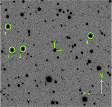
Figure 1. Field of V723 Cas (center) with comparison stars labeled and circled in green. The plate scale is 0515/pixel. North is up and east is to the left.
Download figure:
Standard image High-resolution imageTypically, two comparison stars are used for differential photometry. We initially chose four comparison stars with the understanding that we would use two that showed the least variability. As we prepared our data for publication, comparison stars #3 and #4 were found to be slightly variable over the course of the 10-year observation period. In particular, star #3 often exhibited an amplitude of variation of ∼0.02 mag. During other observing seasons, the amplitude was sometimes as great as ∼0.04 mag. We used the Lomb–Scargle (L–S) method employed by the VARTOOLS Light Curve Analysis Program (Hartman & Bakos 2016) to search the entire 10-year R data set for a period associated with these data. VARTOOLS reports the value of the periodogram at frequency f (in cycles per day), which varies between 0 (for no signal present at all) and 1 (for a perfectly sinusoidal signal). A period of 0.8750443(6) days was detected with a signal strength of 0.4. Comparison star #4 exhibited an amplitude of variation of ∼0.02 in most seasons, occasionally varying as much as ∼0.06 mag. There was no detectable period within the data for star #4. In the final analysis, comparison stars #3 and #4 were excluded from the calculation of differential magnitude, and only comparison stars #1 and #2 were used. These stars were consistently stable, showing variation <0.014 mag.
Atmospheric extinction and transformation coefficients were determined by observing the Landolt (1992) standard field PG+0231 on photometric nights, allowing the instrumental magnitudes of comparison stars #1 and #2 to be placed on the standard photometric system of Landolt (1992). Their B, V, and R magnitudes are tabulated in Table 2. The median error associated with our photometry is determined from the quadratic sum of the error associated with the photometry of V723 Cas and the error associated with the transformation from the local to the standard system as defined by the local photometric sequence.
Table 2. Table of Standardized, Apparent Magnitudes for the Comparison Stars of V723 Cas
| Comparison Star | R.A. J2000.0 | Decl. J2000.0 | B | V | R |
|---|---|---|---|---|---|
| 1 | 01:05:21.58 | +54:01:55.6 | 16.431 ± 0.010 | 15.046 ± 0.007 | 14.241 ± 0.006 |
| 2 | 01:05:20.22 | +54:00:43.2 | 15.539 ± 0.010 | 14.785 ± 0.007 | 14.305 ± 0.006 |
| 3 | 01:05:16.43 | +54:00:46.6 | 15.981 ± 0.010 | 15.083 ± 0.007 | 14.538 ± 0.006 |
| 4 | 01:04:52.61 | +54:01:24.3 | 16.248 ± 0.010 | 15.071 ± 0.007 | 14.377 ± 0.006 |
Download table as: ASCIITypeset image
Our R-band data are presented in Table 3 (available in the machine readable format). B- and V-band observations began in 2007 October and are also available electronically.
Table 3. 2006 October–2016 October R-band CCD Photometry of V723 Cas
| HJD | yyyy mm dd (UT) | R | Rerr |
|---|---|---|---|
| 2454025.5778 | 2006 Oct 17 | 14.739 | 0.007 |
| 2454025.5792 | 2006 Oct 17 | 14.751 | 0.006 |
| 2454025.5806 | 2006 Oct 17 | 14.763 | 0.006 |
| 2454025.5821 | 2006 Oct 17 | 14.774 | 0.006 |
| 2454025.5835 | 2006 Oct 17 | 14.770 | 0.006 |
| 2454025.5875 | 2006 Oct 17 | 14.788 | 0.006 |
| 2454025.5889 | 2006 Oct 17 | 14.790 | 0.006 |
| 2454025.5903 | 2006 Oct 17 | 14.799 | 0.006 |
| 2454025.5918 | 2006 Oct 17 | 14.808 | 0.006 |
| 2454025.5932 | 2006 Oct 17 | 14.790 | 0.006 |
Only a portion of this table is shown here to demonstrate its form and content. A machine-readable version of the full table is available.
Download table as: DataTypeset image
3. Results: The First Two Years
3.1. 2006: The Initial Light Curve
We began our monitoring of V723 Cas in 2006 October in the Bessel R-band, as it contains the  emission line (6562.8 Å), which is often used as an accretion tracer. These data are shown in Figure 2.
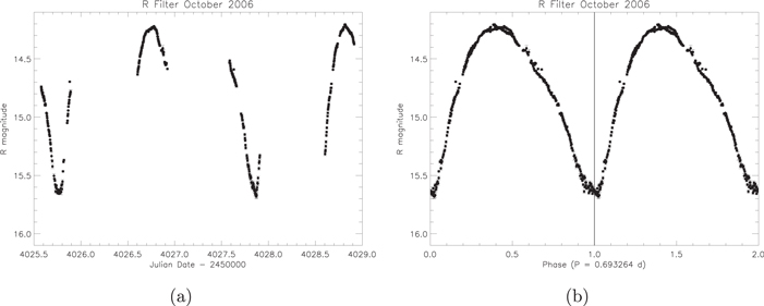
Figure 2. (a) R-band data obtained at the NURO telescope during the nights of UT 2006 October 17–20. (b) The data shown in (a) phased with the orbital period of 0.693264 days.
Download figure:
Standard image High-resolution imageIn Figure 2(a), data obtained each night are plotted, while Figure 2(b) shows those data phased with the orbital period of 0.693264 days, which is discussed further in Section 4 of this paper. These data demonstrate several important features of the V723 Cas light curve that were already known prior to 2006. (1) The saw tooth nature is clearly evident, as had been seen in previous years by several authors starting in 1998 (Chochol et al. 2003; Shugarov et al. 2005; Goranskij et al. 2007). (2) The asymmetry of the light curve is also present. (3) Each epoch (or period) demonstrates some variability, i.e., no two epochs have the exact same light curve, emphasizing the rapidly changing nature of the components that contribute to the light curve (on the order of the orbital period, or roughly 16.6 hr). In particular, the shapes of both the two maxima and two minima for the epochs observed in 2006 October differ significantly. With the phase of minimum set to zero, Goranskij et al. (2007) reported that the phase of maximum light appears between phase 0.3–0.4. However, our 2006 October data do not support this and imply that the maximum light occurs at phase 0.4. Additionally, Goranskij et al. (2007) mentions that at phase 0.6, the light curve shows signs of a slight decline in some cases. Instead of a slight decline, our data show more of a slight "bump" in the light curve.
3.2. BVR Monitoring in 2007
In 2007 October, we began monitoring V723 Cas in the Bessel B, V, and R filters. This allowed us to examine the variation in color as a function of phase. In comparison to the phased R curve from 2006 October (Figure 2), the "bump" on the declining side of the light curve is not as pronounced, appearing near phase 0.8 in these epochs. An interesting "dip" is seen during maximum brightness in all filters, lasting the longest in B. The shape and amplitude of the light curve is very similar in all three bands as reported in Shugarov et al. (2005; see Figure 3).

Figure 3. The top panel shows the R-band data obtained with the NURO telescope from UT 2007 October 15–17. The lower three panels show the B, V, and R data phased with the orbital period of 0.693264 days.
Download figure:
Standard image High-resolution imageThe vertical axis in each plot spans 2 mag in that particular band. The amplitude in the B-band is  mag, in the V-band,
  , and in the R-band,
  . The lower amplitude exhibited by the R-band observations may be explained by the presence of the bright
  (λ = 6562.8 Å) and [Fe x] (λ = 6375 Å) emission lines, which are contained within the R-band filter. The presence of a strong [Fe x] coronal line in the spectra of V723 Cas first appeared in 1999 November (Iijima 2006). Goranskij et al. (2007) reported that the [Fe x] emission line had increased in intensity since its appearance, which suggested that protracted nuclear fusion was taking place at the surface of the WD. Based on the eclipsing nature of this system, and the fact that the [Fe x] emission line arises near the surface of the WD, we expect the amplitude of variations in the R filter to be the lowest compared to the amplitudes in other filters. Interestingly, Ochner et al. (2015) reported that the [Fe x] emission line reached its peak intensity with respect to
  during 2008, after which it began to slowly decline.
4. Photometric Monitoring between 2008–2016: An Evolving Light Curve
We continued to monitor V723 Cas in BVR between 2008 and 2016 and show the R-band light curves (along with 2007) in Figure 4. Unfortunately, due to weather conditions, we were not always able to obtain full coverage of the light curve during our observing runs. Years that were particularly complete are 2007 October, 2008 October, and 2009 January. The B and V data show similar trends and are not plotted here (the data are available electronically).
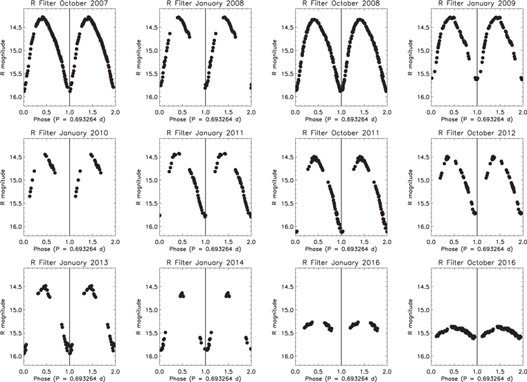
Figure 4. Phased R-band light curves of V723 Cas are displayed for the months and years shown, phased with the orbital period 0.693264 days. Each ordinate spans 2.1 mag to show the dramatic decline in the amplitude between 2014 January and 2016 January.
Download figure:
Standard image High-resolution imageThe general trends that are seen in Figure 4 are as follows. (1) The magnitude of maximum and minimum changes with time, sometimes appearing brighter and sometimes fainter (e.g., compare the minima for 2008 October with that of 2009 January). (2) Beginning in 2011 October, the shape of the maximum starts to change, becoming less rounded and more triangular in shape. The magnitude of maximum has changed from R ∼ 14.3 in 2008 January to R ∼ 14.5 in 2011 October. Between 2011 January and 2012 October, there is an extraordinary change in the magnitude of minimum light, from R ∼ 16.1 in 2011 October to R ∼ 15.7 in 2012.
Perhaps the most striking difference in the light curve of V723 Cas comes between 2014 January and 2016 January. Unfortunately, we have no data for the 2015 observing season. However, on 2015 September 3, Goranskij et al. (2015) reported an abrupt change in the light curve of V723 Cas. Our data confirms this change and our 2016 January data are in agreement with that shown in Goranskij et al. (2015) for 2015 August 7–27. Goranskij et al. (2015) report a new ephemeris and improved period of variability based on the O–C method, which is given by the following formula
Goranskij et al. (2007) suggested that different periods apply to different time intervals based on a trend in the O–C timing of 53 individual minima from their data. Specifically, they concluded that the orbital period of V723 Cas increased with time between 1999 and 2005. Ochner et al. (2015) also reported an ephemeris based on their  photometry:

Using this ephemeris, Ochner et al. (2015) were unable to confirm the O–C trend based on the minima listed in Goranskij et al. (2007), thereby concluding that only one and the same orbital period applies to the whole recorded photometric history of V723 Cas.
We used the L–S method employed by the VARTOOLS Light Curve Analysis Program (Hartman & Bakos 2016) to search our BVR data independently for a period associated with each set of data. The VARTOOLS program calculates the Generalized L–S periodogram of a light curve by generating a spectrum that gives the significance of a periodic signal as a function of frequency or period (Hartman & Bakos 2016). In addition to the detected period, the value of the periodogram at frequency f (in cycles per day) is reported, which varies between 0 (for no signal present at all) and 1 (for a perfectly sinusoidal signal). Two other measures of significance for peaks identified in the periodogram are the logarithm (base 10) of the formal false alarm probability (FAP), and the spectroscopic signal-to-noise ratio (S/N). Our results are reported in Table 4.
Table 4. Periods Associated with the BVR-band Data
| Filter | Period (days) | # of points | Xa | Periodogram Peak | S/N |
|---|---|---|---|---|---|
| B | 0.6932760(1) | 625 | −185.74821 | 0.75608 | 61.01262 |
| V | 0.6932769(8) | 641 | −183.79732 | 0.74371 | 64.83216 |
| R | 0.6932641(6) | 1054 | −319.27984 | 0.75836 | 65.82667 |
Note. The R-band data extends from 2006–2016, while the B and V data range from 2007–2016.
aFAP = 10X.Download table as: ASCIITypeset image
We obtained an epoch based on a time of minimum from one of our 2008 October nights by fitting a fourth-order polynomial to the observations in the R-band. This lead to the following ephemeris for the times of transit through minimum for V723 Cas:

We checked the times of minimum listed in Goranskij et al. (2007) and Ochner et al. (2015) with our ephemeris, and did not find a trend in (O–C)/P (fractions of a period) for either data set. Although we do not see any trends, we provide our photometry (see Table 3) so that it may be combined with other current and future data sets to further search for any potential trends in period evolution. Our data were sufficiently well distributed around at least one minimum in each of the 2006, 2007, 2008 October, and 2013 January observing runs to allow the determination of its epoch. We used the same fitting technique as mentioned above in all cases and derived the following epochs for seven minima (HJD-2450000): 4025.774, 4027.864, 4389.728, 4746.765, 4748.848, and 4750.923, with an uncertainty of ±0.004 days. We checked these times with our ephemeris and saw no trend in (O–C)/P.
In examining our data for times of minima, we noted on several occasions that consecutive minima quite often had variable shapes (see discussion of the 2006 October light curve in Section 3.1). In some cases, there was a flat bottom at minimum. This feature has been observed before and was discussed by Goranskij et al. (2007), who attribute it to a time when the components of the system have different sizes. Specifically, based on their data, Goranskij et al. (2007) suggest that the flat bottom during minimum must form as a result of the transit of the secondary component across the extended accretion disk, whose size exceeds the diameter of the secondary component at that time. They observe that the flat bottom is not constant, implying that the size of the disk must change. Additionally, when the flat bottom does not appear, the decline in brightness at minimum is immediately followed by the rise of the light curve. We also see this phenomena, specifically in the UT 2006 October 19 (JD 2454027.8635) data (see Section 3.1). It is interesting to note that the value of (O–C)/P for this date is −0.9855. Excluding this value, we find an average (O–C)/P value of −0.0074 and a standard deviation of 0.0051 for our times of minima listed above. We accredit this large discrepancy to the fact that what is seen as the minimum in this particular case may not actually be associated with the true Phase 0.0 (i.e., the same orientation of the WD and companion). In other words, it may be that based on the sources of light in the system, such as the accretion disk, an accretion stream and hot spot on the disk, or the irradiated spot on the companion, the combined light from the system continues to diminish even after the WD and companion have moved through phase 0.
The fact that the shape of the minima can be so variable leads us to question how robust the O–C method is for assessing whether or not the orbital period is truly changing for the V723 Cas system.
4.1. Comparison of Our Data with Ochner et al. (2015)
As was mentioned in Section 1, Ochner et al. (2015) also carried out photometric observations of V723 Cas with the  filters, covering 1227 epochs between 2007 November and 2015 March. None of these epochs are coincident with our observations; however, on occasion, they do follow our observations, or occur within the same month as ours. Figure 5 shows the overlap in data for the month of 2008 January in the B filter.
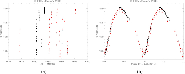
Figure 5. (a) Our B-band data (filled black circles) plotted with B-band data obtained by Ochner et al. (2015) (red triangles). (b) The data from (a) phased with the ephemeris derived in Section 4.
Download figure:
Standard image High-resolution imageConsidering the nature of the rapid variability of the V723 Cas system itself, especially seen during maximum and minimum light on timescales of an orbital period, Figure 5 demonstrates that our observations are in good agreement with those of Ochner et al. (2015) with slightly better signal to noise. While the gross features of the phased light curve, e.g., amplitude, are consistent over long time spans, little details such as the shape of the decline or exact time of minimum or maximum vary on timescales of an orbital period.
Ochner et al. (2015) reported that the mean magnitude during their period of observations was stable at B = 15.75, which is ∼3 mag brighter than in quiescence. Our data do not support this claim. Five distinct seasons of observations (2007 November, 2008 January, 2009 December, 2011 November, and 2013 November) are presented in Figure 2 of Ochner et al. (2015). We downloaded the Ochner et al. (2015) data from the online version of the article and could not locate any data from 2013 November. Thus, we determined that what is plotted, as data from 2013 November in their Figure 2, is actually data from 2013 December. We have data that was obtained in either the month prior to or the month after each of the Ochner et al. (2015) observations presented in Figure 2 of their paper. In Figure 6, we plot our data from 2007–2016 along with that of Ochner et al. (2015). The general decline in both the maximum and mean brightness, as well as a change in amplitude in both data sets can be clearly seen. The bottom plot in Figure 6 shows the mean B magnitude calculated from our data. The error bars in Figure 6 represent the standard deviation associated with the calculation of each average B magnitude, and are thus a representation of the amplitude of the light curve—the larger the error bars, the larger the amplitude.

Figure 6. Top panel: our B-band data (filled black circles) obtained between 2007 and 2016 October plotted with the B-band data obtained by Ochner et al. (2015) (red triangles). Bottom panel: mean B magnitudes calculated from our data shown in the top panel for the same span of time. The error bars represent the standard deviation associated with the calculation of each average B magnitude and represent the amplitude of the light curve during that particular observing run. The dashed green line represents a linear fit to the data. The slope of this line is 0.0004 mag day−1 or 0.15 mag yr−1.
Download figure:
Standard image High-resolution imageWe find that the amplitude in all three filters, while scattered, shows a general decline with time (see Figure 7). The dashed lines represent the general decline in amplitude of the light curve from year to year. There is a dramatic change in amplitude between 2014 and 2016, which was noted by Goranskij et al. (2015). The amplitudes were calculated by simply subtracting the magnitude at minimum light from the magnitude at maximum light. We were unable to calculate an amplitude for 2010 and 2016 January because we did not have complete coverage through either a minimum or a maximum (see Figure 4). These trends were likely missed by Ochner et al. (2015) due to the non-contiguous nature of their observations, as well as the sparse data obtained in the most recent years.
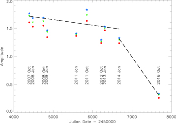
Figure 7. The amplitude of the light curve of V723 Cas in the B (blue solid star), V (green upside down triangle), and R (red circles) filters as a function of time. The dashed lines represent the general decline in amplitude of the light curve from year to year. There is a dramatic change in amplitude between 2014 and 2016.
Download figure:
Standard image High-resolution imageThe report by Goranskij et al. (2015) of the dramatic change in the optical of both the brightness and the amplitude of the light curve was immediately followed by the announcement of X-ray observations indicating that the SSS phase of V723 Cas had come to an end (Ness et al. 2015). Based on their X-ray observations, Ness et al. (2015) estimate that the source turned off some time between 2013 August 19 and 2014 April 1. Our data show that the light curve observed in 2014 January is much different in shape at the maximum when compared to maxima from previous seasons (although, the 2013 January light curve begins to hint at this change to a more pointed maximum; see Figure 4). In order to further investigate this change, we reanalyzed the UV and X-ray data sets available and discuss them in the following section.
5. Ultraviolet and X-Ray Monitoring
Swift (Gehrels et al. 2004) observations of V723 Cas were obtained intermittently between 2006 January and 2014 September while V723 Cas was in the SSS phase. Observations after 2008 September 12 (with the exception of 2014 April 01) were taken using one or more of the UV/Optical Telescope (UVOT; Roming et al. 2005) UV filters. The XRT (Burrows et al. 2005) collected data in Photon Counting (PC) mode throughout all of the observations.
The Swift data have been reprocessed using HEASoft 6.20 and analyzed with the most up-to-date calibration files. UVOT magnitudes were extracted using circles of 5 arcsec radius centered on the source. The XRT data were extracted using a circle of 10-15 pixel radius, depending on the brightness of the source. For both the UVOT and XRT data, the background level was estimated from nearby source-free regions. The results are tabulated in Table 5 and shown in Figure 8. The upper limits plotted in Figure 8 and listed in Table 5 are at the 3σ level. The X-ray source was no longer detected after 2013 August 19, as previously reported by Ness et al. (2015).
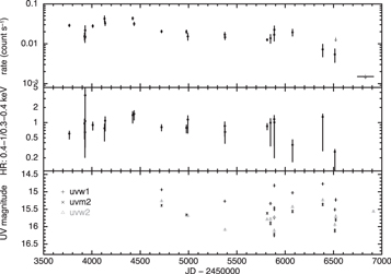
Figure 8. The X-ray light curve is shown in the top panel. The ratio of hard to soft counts (soft: 0.3–0.4 keV; hard: 0.4–1 keV) is shown in the middle panel. The UV magnitudes calculated for each observation are shown in the bottom panel and are given in terms of Vega magnitudes.
Download figure:
Standard image High-resolution imageTable 5. Swift X-Ray and UV Data
| Dates (UT) | JD | ObsID | X-Ray Count s−1 | uvw1 Magnitude | uvm2 Magnitude | uvw2 Magnitude |
|---|---|---|---|---|---|---|
| 2006 Jan 31 | 2453766.7752 | 00030361001 | 0.029 ± 0.002 | ⋯ | ⋯ | ⋯ |
| 2006 Jul 09 | 2453925.6200 | 00030361003 | 0.015 ± 0.003 | ⋯ | ⋯ | ⋯ |
| 2006 Jul 12 | 2453929.2339 | 00030361005 | 0.014 ± 0.004 | ⋯ | ⋯ | ⋯ |
| 2006 Jul 14 | 2453931.1661 | 00030361006 | 0.022 ± 0.007 | ⋯ | ⋯ | ⋯ |
| 2006 Jul 14 | 2453931.1677 | 00030361007 | 0.015 ± 0.002 | ⋯ | ⋯ | ⋯ |
| 2006 Sep 30 | 2454008.9005 | 00030361008 | 0.028 ± 0.002 | ⋯ | ⋯ | ⋯ |
| 2007 Jan 30 | 2454131.4900 | 00030361010 | 0.043 ± 0.007 | ⋯ | ⋯ | ⋯ |
| 2007 Feb 06 | 2454138.3059 | 00030361011 | 0.033 ± 0.004 | ⋯ | ⋯ | ⋯ |
| 2007 Nov 18 | 2454423.0987 | 00030361012 | 0.043 ± 0.003 | ⋯ | ⋯ | ⋯ |
| 2007 Dec 03 | 2454437.7596 | 00030361013 | 0.032 ± 0.003 | ⋯ | ⋯ | ⋯ |
| 2008 Sep 12 | 2454721.5124 | 00030361014 | 0.020 ± 0.001 | 14.94 ± 0.02 | 15.39 ± 0.02 | 15.27 ± 0.02 |
| 2009 May 27 | 454978.9339 | 00090244001 | 0.019 ± 0.001 | ⋯ | 15.66 ± 0.02 | |
| 2009 Jun 11 | 2454993.5262 | 00090244002 | 0.015 ± 0.003 | ⋯ | ⋯ | 15.69 ± 0.03 |
| 2010 Jun 28 | 2455375.5991 | 00030361016 | 0.017 ± 0.002 | 15.27 ± 0.02 | ⋯ | ⋯ |
| 2010 Jun 30 | 2455378.2173 | 00030361017 | 0.015 ± 0.002 | 16.09 ± 0.01 | ⋯ | ⋯ |
| 2011 Sep 09-10 | 2455813.5272 | 00030361018 | 0.013 ± 0.001 | ⋯ | 15.62 ± 0.02 | 15.79 ± 0.02 |
| 2011 Oct 14 | 2455848.6230 | 00045766001 | 0.013 ± 0.003 | 15.34 ± 0.03 | 15.91 ± 0.04 | 15.78 ± 0.04 |
| 2011 Nov 21 | 2455887.0738 | 00045766002 | 0.017 ± 0.005 | 15.74 ± 0.04 | 16.23 ± 0.06 | 16.12 ± 0.05 |
| 2011 Nov 22 | 2455888.0773 | 00045766003 | 0.023 ± 0.005 | 14.82 ± 0.03 | 15.48 ± 0.05 | 15.73 ± 0.03 |
| 2012 May 29 | 2456076.6028 | 00045766004 | 0.019 ± 0.004 | 14.94 ± 0.02 | 15.39 ± 0.02 | 15.27 ± 0.02 |
| 2013 Apr 06 | 2456389.3659 | 00049546001 | 0.007 ± 0.002 | 14.77 ± 0.03 | 15.36 ± 0.04 | 15.24 ± 0.03 |
| 2013 Aug 09-10 | 2456513.9448 | 00049546002 | 0.005 ± 0.002 | 15.51 ± 0.03 | 16.12 ± 0.04 | 15.95 ± 0.04 |
| 2013 Aug 19 | 2456524.4255 | 00049546003 | <0.013 | 15.23 ± 0.04 | 15.79 ± 0.06 | 15.71 ± 0.04 |
| 2014 Apr 01 | 2456748.7361 | 00091926001 | <0.002 | ⋯ | ⋯ | ⋯ |
| 2014 Sep 13 | 2456914.0744 | 00049546004 | <0.002 | ⋯ | ⋯ | 15.57 ± 0.02 |
Download table as: ASCIITypeset image
The X-ray spectra (Figure 9) were fitted with an absorbed plane-parallel, static, non-local-thermal-equilibrium stellar atmosphere model (grid 003).7 Observations were required to have at least 50 spectral counts to be included in the fitting; data were merged between 2011 September and November and again from 2013 April to August to obtain sufficient spectral counts at these times. Only data with energies below 1 keV were modeled, as there were very few counts at higher energies; there was, therefore, no need for a second component, as is sometimes needed to account for the underlying shock emission in novae. The absorbing column was fixed at the ISM value of 2.35 × 1021 cm−2 (Schwarz et al. (2011); the statistical quality of the spectra was not high enough to provide useful constraints on any variation in the column density), and the luminosity in the bottom panel of Figure 9 was calculated assuming a distance of 3.85 kpc (Lyke & Campbell 2009).
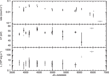
Figure 9. Parameters from the atmosphere model fits to the X-ray spectra. The middle panel shows the temperature, while the bolometric luminosity of this component (assuming a distance of 3.85 kpc) is plotted in the bottom panel.
Download figure:
Standard image High-resolution imageThe X-ray and UV data shown in Figure 8 were phased using the ephemeris derived in Section 4. The three UV filters and X-ray data were folded separately. Where there are multiple snapshots of data within one ObsID, they were included individually for the phase folding (always for the UV; when there was a detection in the X-ray).
Figure 10 shows that the orbital modulation observed in the optical is also seen in the UV and X-ray. The UV maximum and minimum occur at roughly the same phases as observed in the optical (see Section 3.1). However, the periodic maximum and minimum of the X-ray modulation is slightly out of phase with the variations seen in both the optical and UV. The X-ray maximum occurs near phase 0.5, while the minimum occurs between phases 0.8–0.9. Orbital modulation of both X-ray and UV data have also been seen in the classical novae, HV Cet (Beardmore et al. 2012) and V959 Mon (Page et al. 2013), as well as the recurrent nova, LMC 2009a (Bode et al. 2016).
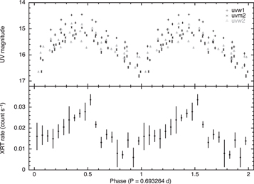
Figure 10. The phased UV light curve is shown in the top panel, while the phased X-ray data are shown in the bottom panel.
Download figure:
Standard image High-resolution imageTo begin to understand and interpret these results, we recall that a common feature of all compact binary SSSs is a high disk rim (up to  ) produced by the impact of an accretion stream. The rim is irradiated by the central WD and can act like a large screen, both obscuring and reflecting light within the system. Reprocessed X-ray radiation from the WD by this extended region dominates the flux in both the UV and optical (Meyer-Hofemeister et al. 1997; Schandl et al. 1997). The difference in phases of maximum and minimum between the UV/optical and X-rays suggests a different origin of emission. While the UV flux is a result of the reprocessed X-ray radiation as mentioned above, the reprocessing site must have a slightly different view of the X-ray source than we do. In fact, it is possible that shielding from the disk rim may explain the "low" value of X-ray luminosity (
 erg s−1) observed (see Figure 9). In the following section, we model the optical light curves by using an eclipsing binary modeling program, complete with an accretion disk, accretion disk hot spot, and an irradiated secondary.
6. Modeling the V723 Cas System
We attempted to model the V723 Cas system and initial light curves with the eclipsing binary modeling program Nightfall, written by Rainer Wichmann.8 Basic data about the system was collected and used as the initial input. These data are listed in Table 6.
Table 6. Measured V723 Cas System Parameters
| Parameter | Value | References |
|---|---|---|
| Quiescent B mag | 18.58 ± 0.1 | Goranskij et al. (2007) |
| Distance |

|
Lyke & Campbell (2009) |
| Inclination Angle | 62 0 ± 15 0 ± 15 |
Lyke & Campbell (2009) |

|
0.6 ± 0.1 | Gonzalez-Riestra et al. (1996)a |
| AV | 1.9 ± 0.3 | Evans et al. (2003) |
| WD Mass |

|
Evans et al. (2003) |
Note.
aSee discussions regarding the interstellar reddening estimates by Evans et al. (2003) and Iijima (2006).Download table as: ASCIITypeset image
There is no known information about the donor star in the V723 Cas system. As such, we assumed the companion to have a mass of  (which makes the mass ratio = 1.0) and a temperature T = 4500 K. These choices correspond to a spectral type of K5 (Cox 2000). The assumed mass for the companion is supported by calculations performed by Politano (1996) that identify a mass range for the donor star in cataclysmic variable systems that support stable mass accretion. We assumed that mass transfer was occurring within the system and that the companion had filled its Roche lobe. Additionally, an accretion disk with a hot spot was placed around the WD. We consulted Djurašević (1996) and Smak (2002) for estimates of accretion disk parameters. Free parameters consisted of the placement, brightness, and size of an irradiated spot on the companion, as well as the location, temperature, and extent of a hot spot on the edge of the accretion disk for the majority of the model dates. Additionally, we found it necessary to change the size of the accretion disk.
We started by modeling the 2006 October light curve. The results are shown in Figure 11, where the model is represented by a solid red line. Phase 0.0 is taken to be when the companion star is directly in front of the WD/accretion disk as viewed from the Earth (Figure 11, Image (a)). The steep rise in brightness seen in the light curve can be accounted for by the proper placement of the accretion disk hot spot and a spot on the secondary due to the irradiance by the WD/accretion disk hot spot. As the system moves through phase 0.4, the irradiated spot on the secondary and the WD/accretion disk are nearly fully in view, resulting in the observed peak brightness (Figure 11, Image (b)). Between phases 0.8 and 1.0/0.0, the model deviates substantially from the observed data. We suspect that this could be due to "the neck" of the accretion stream, which cannot be modeled using Nightfall.

Figure 11. Images (a)–(d) are model representations of the V723 Cas system for specific phases identified in the light curve. The 2006 October light curve in R (black circles), phased with the ephemeris derived in this paper, along with the model fit (solid red line) is shown. An arbitrary offset in magnitude of 14.25 is added to the model to bring it in line with the actual data. It should be noted that the irradiated spot appears as a white area on the surface of the secondary. As a result, images (a) and (b) do not show the outline of the star's actual shape.
Download figure:
Standard image High-resolution imageWe found that we could easily model the light curves of additional years/months using some of the same parameters, which gave us confidence in our choices. It should be noted that we only qualitatively assessed the goodness of fit using a chi "by eye" due to the variable nature of the light curve itself. We report our values in Table 7 as examples of successful models that are consistent with the expectations of the components in the V723 Cas system. We acknowledge that the parameter values listed are not necessarily unique. For example, we were able to achieve roughly the same model for the 2009 January light curve using an outer radius of the disk = 0.6, the longitude of the accretion hot spot 125° and its extent = 80°, with the latitude of the companion's spot = 0°, its longitude = 70°, and its radius = 50°. All other parameters were left the same, because changing them resulted in a large deviation from the shape of the light curve. The location of the hot spot on the rim of the accretion disk is particularly sensitive to matching the minimum observed at phase 0. For each light curve (separated by season), we varied the size of the accretion disk, the location and size of the accretion hot spot, and the location and size of the irradiated spot on the companion. It should be noted that the program Nightfall refers to the star that is eclipsing first, i.e., the star that passes in front of the other one at orbital phase zero, as the primary star. Therefore, the star that is eclipsed first is considered the secondary (Nightfall User Manual). This is inverse to the usual convention. Thus, the mass ratio used in our models is technically  , where M1 = the mass of the WD and M2 = the mass of the secondary, which we have referred to as the companion throughout this paper. In any case, we simply show that the components included seem to model the observed data fairly well.
Table 7. Nightfall Model Parametersa
| Oct 06 | Oct 07 | Jan 08 | Oct 08 | Jan 09 | Jan 11 | Oct 11 | Oct 12 | Jan 16 | Oct 16 | ||
|---|---|---|---|---|---|---|---|---|---|---|---|
| Basic: | Parameter | Value | Value | Value | Value | Value | Value | Value | Value | Value | Value |
| Companion Fill Factorb | 1.0 | 1.0 | 1.0 | 1.0 | 1.0 | 1.0 | 1.0 | 1.0 | 0.9 | 0.9 | |
| T of WD | 300,000 K | 300,000 K | 300,000 K | 300,000 K | 225,000 K | 225,000 K | 225,000 K | 120,000 K | 120,000 K | 120,000 K | |
| Disk: Reprocessingc | |||||||||||
| Outer Radiusd | 0.84 | 0.86 | 0.92 | 0.79 | 0.62 | 0.64 | 0.59 | 0.57 | 0.61 | 0.58 | |
| Temperature of Hot Spot | 20,000 K | 20,000 K | 20,000 K | 20,000 K | 20,000 K | 20,000 K | 20,000 K | 18,000 K | |||
| Puffiness of Hot Spotf | 0.1 | 0.1 | 0.1 | 0.1 | 0.1 | 0.1 | 0.1 | 0.1 | |||
| Longitude of Hot Spot | 1155 |
1185 |
1163 |
1177 |
1221 |
1199 |
1329 |
1361 |
|||
| Extent of Hot Spot | 821 |
685 |
768 |
672 |
648 |
661 |
812 |
777 |
|||
| Depth of Hot Spotg | 0.15 | 0.15 | 0.15 | 0.15 | 0.15 | 0.15 | 0.15 | 0.15 | |||
| Spot on Companion: | |||||||||||
| Longitude | 543 |
442 |
535 |
557 |
505 |
515 |
577 |
514 |
310 |
||
| Latitude | 209 |
94 |
186 |
152 |
59 |
86 |
117 |
203 |
695 |
||
| Radius of spot | 500 |
418 |
508 |
533 |
531 |
563 |
503 |
540 |
234 |
||
| Dimfactor, APh | 1.69 | 1.52 | 1.59 | 1.44 | 1.41 | 1.46 | 1.42 | 1.36 | 0.82 | ||
Notes.
aThe following parameters are held constant for all models with definitions listed below: q = 1, defined as , i = 62°, the WD fill factorb = 0.007, the inner radiusd of the accretion disk = 0.15, the thicknesse of the disk = 0.005.
bThe fill factor is given in terms of the Roche lobe.
cFor a reprocessing disk, the temperature falls off with radius as
, i = 62°, the WD fill factorb = 0.007, the inner radiusd of the accretion disk = 0.15, the thicknesse of the disk = 0.005.
bThe fill factor is given in terms of the Roche lobe.
cFor a reprocessing disk, the temperature falls off with radius as  .
dThis is given in terms of the size of the WD Roche lobe.
eThis is the thickness at the inner edge of the disk. The height of the disk at radius r is computed as
.
dThis is given in terms of the size of the WD Roche lobe.
eThis is the thickness at the inner edge of the disk. The height of the disk at radius r is computed as  . For the reprocessing disk, a = 0.0, b is chosen such that at the inner disk radius, the disk thickness equals the thickness input parameter. The exponent c is set to
  , which is the correct value for a reprocessing disk (taken from the Nightfall User Manual).
fThis is in the same units as the disk size and is added to the the disk height at the hot spot center on the outer rim.
gThis is measured as a fraction of the disk size and extends inward from the outer edge of the disk.
h
, which is the correct value for a reprocessing disk (taken from the Nightfall User Manual).
fThis is in the same units as the disk size and is added to the the disk height at the hot spot center on the outer rim.
gThis is measured as a fraction of the disk size and extends inward from the outer edge of the disk.
h
 , which represents the ratio of the (local) temperature TP with spot to the temperature T without spot (taken from the Nightfall User Manual).
Download table as: ASCIITypeset image
The amplitude of the 2009 January light curve was significantly different (smaller) from the 2006–2008 light curves (see Figure 4). In order to model this change, we had to cool the WD to a temperature of T = 225,000 K. Although we did not specifically model the light curve from 2010 January due to lack of data, the 2009 January model parameters seemed to be able to fit those data, as well as the data from 2011 January, needing only to modify the location and extent of the accretion hot spot and the spot on the companion slightly. In order to fit the data for 2012 October, we had to cool the WD to a temperature of T = 120,000 K. We found it nearly impossible to model the light curves that were obtained in 2013 and 2014 January. As noted in Section 4, the shape of the light curve maximum at this time changed from somewhat rounded to a more triangular shape. We were unable to recreate this shape using Nightfall.
The next major change in the light curve was announced by Goranskij et al. (2015) and is observed in our 2016 January data (see Figure 4). These data were successfully modeled by shrinking the companion to 0.9 (just inside its Roche lobe) and adding a slightly cooler spot to the companion. Because we do not have full coverage of the light curve, it was hard to tell exactly what was happening around phase 0.5. We found that we could easily model the 2016 January data by leaving the accretion disk parameters roughly as they had been (outer radius = 0.6; inner radius = 0.15), and removing the accretion disk hot spot altogether. In order to model the data from 2016 October, there was no need for a cooler spot on the companion. We show a sample of models and light curves in Figure 12. The fact that V723 Cas was not detected in the X-ray after 2013 August 19 (see Section 5 and Ness et al. 2015) suggests that hydrogen burning on the surface of the WD had likely ceased. This could imply that the accretion rate decreased significantly and that the accretion disk (and hot spot) is no longer the dominant source of optical light.
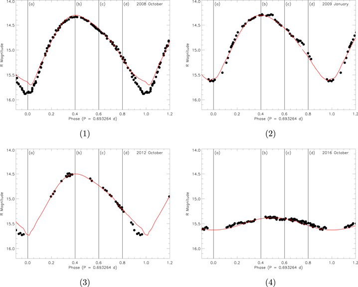
Figure 12. The 2008 October (1), 2009 January (2), 2012 October (3), and 2016 October (4) light curves in R (black circles), phased with the ephemeris derived in this paper, along with the model fits (solid red line). The parameters used to model each season are given in Table 7.
Download figure:
Standard image High-resolution imageWe note that there could, in fact, be several parameters that may be used as inputs for Nightfall that may also adequately model the V723 Cas light curves observed between 2006 and 2016. We report our values as an example of a successful model that are consistent with the expectations of those for the V723 Cas system.
7. The Color Evolution From 2007 to 2016
As noted in Section 3.2, observations of V723 Cas in B, V, and R were made sequentially in time, with each exposure lasting 180 s. Including the readout time and a filter change, the total time in between each measurement was 3.17 minutes. In order to calculate a B − V or a V − R color, corresponding sequential BVR observations were identified. The V magnitude was subtracted from the B magnitude in the sequence, and an average Julian date was calculated from the times of the observations. Similarly, a V − R color was determined. The results of our calculations are shown in Figure 13 for 2007/2008 October. The error bars come from adding in quadrature the individual magnitude errors associated with each B, V, or R measurement.
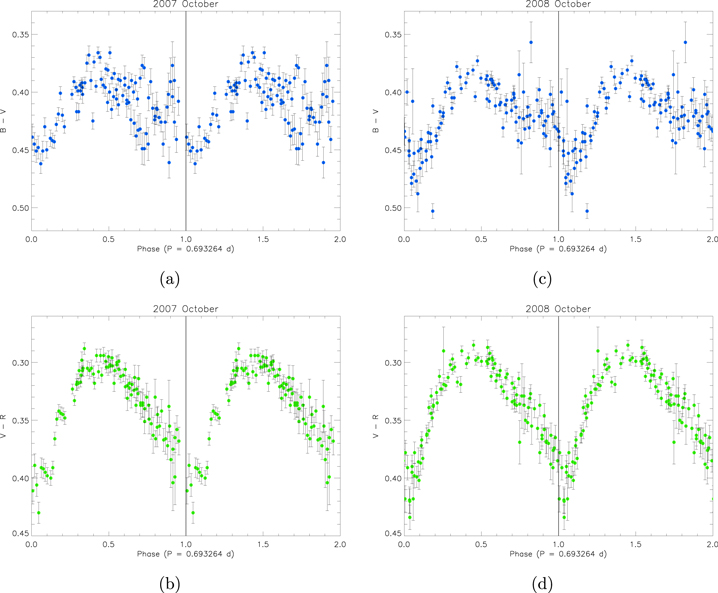
Figure 13. (a) The B − V data obtained with the NURO telescope from UT 2007 October 15–17. (b) The V − R data obtained from UT 2007 October 15–17. (c) The B − V data obtained from UT 2008 October 7–11. (d) The V − R data obtained from UT 2008 October 7–11. All data has been phased with the ephemeris derived in Section 4.
Download figure:
Standard image High-resolution imageThe 2007/2008 color values are similar to the color indices of Goranskij et al. (2007) obtained throughout 2002 while the V723 Cas system was in the nebular phase. They combined both photoelectric UBV observations and BVRI CCD photometry to produce their color versus phase curves. They report seeing weak orbital variation in almost all colors except U − B, which was attributed to the lower accuracy of the U-band observations. In 2002, while the system was still in the nebular phase, the amplitude of the variations in B − V and V − R were reported to be ∼0.15 mag. During minimum light, the system became redder in the B − V and V − R colors (Goranskij et al. 2007).
Our observations in Figure 13 reveal a clear trend in color variation as a function of phase. The B − V color has an amplitude of roughly 0.07 mag, while the V − R color shows an amplitude of ∼0.15 mag. These colors represent observations that were made over the course of three consecutive epochs (see Figure 3, top panel for reference). In agreement with Goranskij et al. (2007), the general trend is for the color to become bluer as maximum light is approached (for our observations near phase 0.4) and then redder as the system heads into minimum light (phase 0/1). However, as the system moves through phase 0/1, both colors continue to get redder until they abruptly begin to exhibit bluer values around phase 0.15/1.15. Additionally, there appears to be an interesting feature in the B − V data occurring between phase 0.85 and 1.0. The B − V value exhibits a shift toward bluer colors during those phases. Coincidentally, this is also the phase where we see a minimum in the X-ray data (see Figure 10).
Goranskij et al. (2007) attributed the trend seen in color with orbital phase as due to temperature variations across the surface of the distended companion and/or a hot spot on the accretion disk. This trend continued with the same amplitude of variation in both B − V (from ∼0.38 at maximum to ∼0.45 at minimum with a mean of 0.41) and V − R (from ∼0.30 at maximum to ∼0.40 at minimum with a mean of 0.34 ) until 2011 October.
In 2011 October, the system exhibited a pronounced change in both B − V and V − R, as is demonstrated in Figure 14, left panel. The B − V value moved toward a bluer mean value of ∼0.28, while the V − R value moved toward a redder mean value of ∼0.45. Surprisingly, in 2012 October, the mean B − V value was ∼0.68, while the mean V − R color (∼0.44) remained close to its 2011 October value (see Figure 14, right panel). Additionally, the variation as a function of phase that was seen in previous years moderated substantially, and the B − V color variation appeared to be more random in nature.
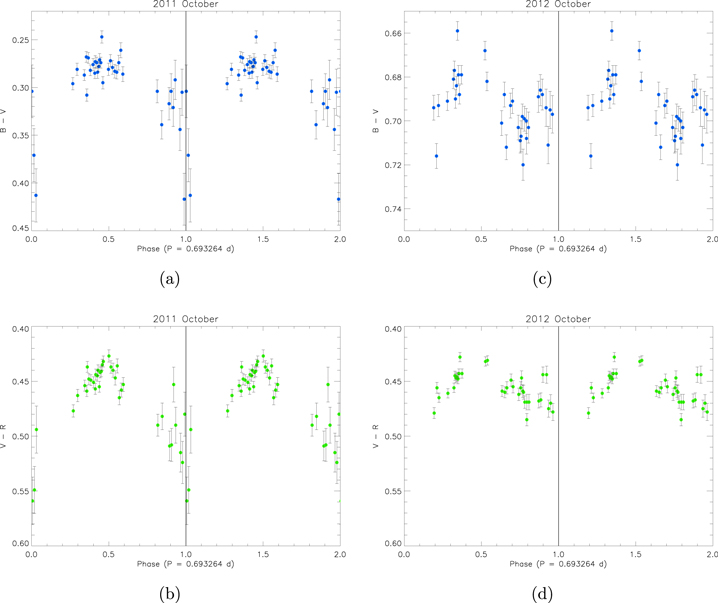
Figure 14. (a) The B − V data obtained with the NURO telescope from UT 2011 October 16–19. (b) The V − R data obtained from UT 2011 October 16–19. (c) The B − V data obtained from UT 2012 October 14–17. (d) The V − R data obtained from UT 2012 October 14–17. All data has been phased with the ephemeris derived in Section 4.
Download figure:
Standard image High-resolution imageThe B − V color exhibited a shift back to a bluer mean value of ∼0.27 in 2014 January, similar to that which was seen in 2011 October, returning to a B − V value of ∼0.77 the next time we observed it in 2016 January. To demonstrate these changes in overall average color, we created a plot of mean color for each season. This is shown in Figure 15. The excursion to bluer B − V colors, as well as a global change in colors, can be easily seen.
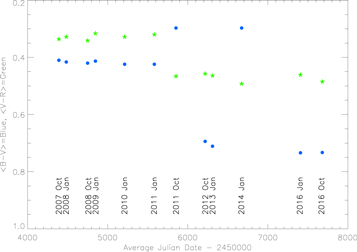
Figure 15. The mean B − V (blue dots) and V − R (green stars) colors for all observing seasons.
Download figure:
Standard image High-resolution image
8. Conclusions
We have observed V723 Cas photometrically between 2006 and 2016. We have shown that:
- 1.the optical light curves exhibit variability on timescales as short as 16 hr (from epoch to epoch), as well as yearly changes that have resulted in a general decline in the overall brightness of the system;
- 2.the amplitude of the light curve has been variable, and has changed significantly between 2014 January when the amplitude of variation was ∼1.3 to ∼0.3 in 2016 October;
- 3.in 2016, the light curve was roughly sinusoidal in shape, with the maximum occurring at phase 0.5 and the minimum at phase 0, as would be expected in a standard eclipsing binary system;
- 4.the UV and X-ray data are modulated by the orbital period, and that the UV data roughly follow the same variation seen in the optical (until 2016) with the maximum occurring at phase 0.4 and minimum at phase 0; and
- 5.the X-ray maximum occurs at phase 0.5, with minimum at phase 0.9 suggesting a different origin of emission for the X-rays. Because the UV flux is a result of the reprocessed X-ray radiation, the reprocessing site must have a slightly different view of the X-ray source than we do.
Our modeling suggests that the presence of an accretion disk and an accretion hot spot, in addition to an irradiated companion are necessary in order to model the shape of the light curves; subtle differences in the light curve from epoch to epoch can be explained by variations in the shape of the rim of the accretion disk. Additionally, the evolution of the light curves over the course of the past 10 years suggests that the WD is cooling. This is supported by the lack of observable X-rays after 2013 August (Ness et al. 2015), as well as the observed declining emission of the [Fe x] 6375 Å coronal line (Ochner et al. 2015), which suggests that nuclear burning on the surface of the WD has most likely come to an end.
We would like to thank the anonymous referee and the scientific editor for helping us improve this paper. The authors from Dickinson College would like to acknowledge and thank the Dean's Office for supporting Dickinson's partnership in NURO (until 2016), which has allowed 28 undergraduates between 2006 October and 2016 October to gain hands-on experience at a professional observatory. We especially thank the following students for taking the data that was analyzed and presented in this paper: Kristin Jekielek, Kristina Gaff Johnson, Karen Younkins, James Martin, Francis Cressotti, Kelli Mauer, James Doyle, Anubhav Mohan, Stephanie Conant, Mara Anderson, Christine Welling, Matthew Gallentine, Sophia Flury, Justin Brown, Olivia Lanes, Justin Garder, and Alaina Einsig. We also thank our colleagues, Dr. Karen Lewis and Dr. Windsor Morgan for taking the students to NURO and observing V723 Cas for this project. C.M.H.D. acknowledges support for herself and a subset of the aforementioned undergraduates from the Student-Faculty Research Funds, as well as the NAU NASA Space Grant, specifically used for student travel funds. K.L.P. acknowledges support from the UK Space Agency.
Footnotes
- 5
This information was taken from the NURO website: http://www.nuro.nau.edu/specs.htm.
- 6
IRAF is distributed by the National Optical Astronomy Observatories, which are operated by the Association of Universities for Research in Astronomy, Inc., under cooperative agreement with the National Science Foundation.
- 7
TMAP: Tübingen NLTE Model Atmosphere Package: http://astro.uni-tuebingen.de/~rauch/TMAF/flux_HHeCNONeMgSiS_gen.html.
- 8