


Abstract
We report on the improved ephemerides for the irregular Jovian satellites. We used a combination of numerically integrated equations of motion and a weighted least-squares algorithm to fit the astrometric measurements. The orbital fits for 59 satellites are summarized in terms of state vectors, post-fit residuals, and mean orbital elements. The current data set appears to be sensitive to the mass of Himalia, which is constrained to the range of GM = 0.13–0.28 km3 s−2. Here, GM is the product of the Newtonian constant of gravitation, G and the body's mass, M. Our analysis of the orbital uncertainties indicates that 11 out of 59 satellites are lost owing to short data arcs. The lost satellites hold provisional International Astronomical Union (IAU) designations and will likely need to be rediscovered.
Export citation and abstract BibTeX RIS
1. Introduction
The irregular satellites of giant planets are a diverse population of relatively small objects that reside in orbits with high inclinations and eccentricities (Nicholson et al. 2008). Although still dominated by the gravitational field of the host planet, orbits of these satellites have large semimajor axes that place them under a strong influence of gravitational perturbations from the Sun. The general consensus is that the irregular satellites did not form "in situ" but were captured in the early history of the solar system (Saha & Tremaine 1993; Gladman et al. 2001; Asthakov et al. 2003; Nesvorný et al. 2007; Vokrouhlický et al. 2008; Philpott et al. 2010; Gaspar et al. 2011). Their dynamical properties provide a window into the capture mechanisms and the role that resonances played in orbital stability (Carruba et al. 2002; Nesvorný et al. 2003). Jupiter has 59 known irregular satellites, of which seven are in prograde orbits, while the rest are retrograde. A number of satellites appear to be clustering in the orbital element space, suggesting a common origin (Nesvorný et al. 2004; Beaugé & Nesvorný 2007). Besides the prograde Himalia's group, there seem to be three more retrograde satellite families: Carme's, Ananke's, and Pasiphae's.
The analysis presented in this paper is an extension of orbital fits discussed in Jacobson (2000) and Jacobson et al. (2012). Jacobson (2000) was published before a large number of irregular Jovian satellites were discovered in the early 2000s (Sheppard & Jewitt 2003). It reported on the orbital analysis of eight satellites: Himalia, Elara, Lysithea, Leda, Pasiphae, Sinope, Carme, and Ananke. These orbital fits were used to support science planning of NASA's Galileo mission. Emelyanov (2005a) had an updated orbital estimate for 54 irregular satellites in 2005, but there have been new astrometric measurements and five new satellites discovered in the past 11 yr. The Jacobson et al. (2012) analysis contained all 59 satellites, but the manuscript focused on recovery observations and estimation of the plane-of-sky orbital uncertainties as opposed to an overall evaluation of the orbital fits. The analysis discussed in this paper contains observations though 2016, and we focus on state vectors, post-fit residuals, mean elements, and the orbital uncertainties. We also investigated the data sensitivity to the satellite masses.
2. Methods
2.1. Orbital Fit
Orbits of the irregular Jovian satellites are strongly perturbed by the Sun and cannot be entirely described by an analytical theory. In order to obtain high-precision satellite ephemerides, we numerically integrated equations of motion as described in Peters (1981). The equations are defined in Cartesian coordinates, with Jovian system barycenter as the origin. The axes are referenced to the International Celestial Reference frame (ICRF). We used barycentric dynamical time (TDB) to remain consistent with Jet Propulsion Laboratory (JPL) planetary ephemerides. The gravitational field of Jupiter includes the zonal harmonic coefficients J2, J3, J4, and J6. The model includes the perturbations from the Galilean satellites, Saturn, Uranus, Neptune, and the Sun. The mass of the Sun was modified to include the terrestrial planets and the Moon. We used JPL's satellite ephemeris JUP310 (Jacobson, unpublished) for the positions of the Galilean satellites. JPL's planetary ephemeris DE435 (Folkner 2014) was used for the positions of the Sun and planets. The complete list of dynamical constants used in our integration is shown in Table 1.
Table 1. Dynamical Constants Used in the Orbit Integration
| Name | Value |
|---|---|
| Jovian system GM (km3 s−2)a | 126,712,764.8 |
| Saturnian system GM (km3 s−2)b | 37,940,585.2 |
| Uranian system GM (km3 s−2)c | 5,794,557.0 |
| Neptune system GM (km3 s−2)d | 6,836,527.1 |
| Sun GM (km3 s−2)e | 132,713,233,263. |
| Io GM (km3 s−2)f | 5959.9 |
| Europa GM (km3 s−2)f | 3202.7 |
| Ganymede GM (km3 s−2)f | 9887.8 |
| Callisto GM (km3 s−2)f | 7179.3 |
| Jupiter radius (km)a | 71,492. |
| Jupiter J2a | 1.4696 × 10⁻² |
| Jupiter J3a | −6.4 × 10⁻⁷ |
| Jupiter J4a | −5.871 × 10⁻⁴ |
| Jupiter J6a | 3.43 ×10⁻⁵ |
| Jupiter pole R.A.a(deg) | 268.06 |
| Jupiter pole decl.a(deg) | 64.50 |
| Jupiter pole R.A. ratea (deg cy−1) | −0.0065 |
| Jupiter pole decl. ratea (deg cy−1) | 0.0024 |
Notes.
aJUP230 solution; R. Jacobson, unpublished. bJacobson et al. (2006). cJacobson et al. (1992). dJacobson (2009). eFolkner et al. (2014), Sun GM augmented with the masses of the inner planets. fJUP310 solution; R. Jacobson, unpublished.Download table as: ASCIITypeset image
The integration used a variable size time step and the variable-order Gauss–Jackson method. We imposed a maximum velocity error of 10−10 km s−1 in order to control the integration step size. As a result, the average integration step size was ∼4800 s. We used a weighted least-squares procedure based on Householder transformations (Lawson & Hanson 1974) to adjust the epoch state vectors for the satellites. The GMs, the products of the Newtonian constant of gravitation G and the satellites masses M, were initialized at 10−20 km3 s−2 but were otherwise allowed to adjust.
2.2. Data
The long data arc and good quality of astrometric measurements are the prerequisites for high-precision orbital determination. Most of the irregular Jovian satellites have periods of about 2 yr, which makes it relatively easy to acquire good orbital coverage. However, many of these objects are faint, H > 23 mag, which puts a requirement on large telescopes as the observing instruments.
Astrometric observations for the first-discovered Jovian irregulars, Himalia, Elara, Pasiphae, and Sinope, date back to the late nineteenth and early twentieth centuries, and long data arcs also exist for Lysithea, Carme, and Ananke. The rest of the satellites were discovered relatively recently, in the early 2000s, and some of them have not been reobserved since their discovery. Jacobson et al. (2012) described the efforts to recover some of the satellites that were considered to be nearly lost, and in the process, two more Jovian irregulars were discovered (Alexandersen et al. 2012).
The large majority of astrometric observations originate from Earth-based telescopes, although there are a handful of observations of Himalia and Callirrhoe from the New Horizons spacecraft flyby of Jupiter. The modern Hipparcos Catalog (Perryman et al. 1997) based astrometry is reported as positions in the ICRF. We convert the older measurements to the ICRF positions. The references to optical observations up to the year 2000 are documented in Jacobson (2000). We continued to use the Jacobson (2000) observational biases for the early measurements. We have since extended the data set with observations published in the Minor Planet Electronic Circulars (MPEC), the International Astronomical Union Circulars (IAUC), the Natural Satellites Data Center (NSDC) database (Arlot & Emelyanov 2009), the United States Naval Observatory Flagstaff Station catalog (www.nofs.navy.mil/data), and the Pulkovo Observatory database (www.puldb.ru/db). An extensive data set spanning 23 yr of observation of 18 irregular satellites (12 Jovian satellites) has been published in 2015 by Gomes-Júnior et al. (2015).
Our resulting data set contains more than 30,000 astrometric points from over 100 observatories. The measurements were weighted by either observer-assigned uncertainties or revised uncertainties that were scaled by an inverse of the rms of the residuals for a particular observer.
3. Results
3.1. Post-fit Residuals
Table 2 shows the time span and number of points used in orbital fits, as well as the post-fit residual statistics. We list the rms of the post-fit residuals in right ascension (R.A.) and declination (decl.) in units of arcseconds and in units of standard deviation, σ. The residuals of 0 5 are expected for orbital fits to faint, distant objects such as the irregular Jovian satellites. Our weighting scheme intended to bring the rms of the residuals converted to the units of standard deviation close to 1σ. Some of the reduced values in Table 2 are smaller because we did not weight the data below the star catalog errors, which are estimated to be around 030.
Table 2. Post-fit Residual Statistics
| Satellite | Time Span | No. | rms | Reduced rms | ||
|---|---|---|---|---|---|---|
| R.A. | decl. | R.A. | decl. | |||
| Himalia | 1894–2016 | 3257/3251 | 0410 |
0373 |
0.632σ | 0.619σ |
| Elara | 1905–2016 | 1877/1876 | 0372 |
0365 |
0.692σ | 0.710σ |
| Lysithea | 1938–2016 | 772 | 0357 |
0317 |
0.727σ | 0.690σ |
| Leda | 1974–2015 | 308/309 | 0432 |
0396 |
0.755σ | 0.738σ |
| Dia | 2000–2011 | 64 | 0368 |
0395 |
0.789σ | 0.848σ |
| Themisto | 1975–2015 | 104 | 0551 |
0412 |
0.827σ | 0.751σ |
| Carpo | 2003–2009 | 39 | 0313 |
0294 |
0.832σ | 0.960σ |
| Ananke | 1951–2015 | 1042/1043 | 0399 |
0456 |
0.795σ | 0.802σ |
| Harpalyke | 2000–2011 | 84 | 0409 |
0343 |
0.916σ | 0.842σ |
| Iocaste | 2000–2015 | 78 | 0348 |
0408 |
0.931σ | 1.008σ |
| Praxidike | 2000–2016 | 70 | 0216 |
0330 |
0.719σ | 0.952σ |
| Thyone | 2001–2003 | 30 | 0204 |
0319 |
0.680σ | 0.886σ |
| Hermippe | 2001–2011 | 49 | 0329 |
0330 |
0.840σ | 0.820σ |
| Euanthe | 2001–2009 | 23 | 0258 |
0138 |
0.822σ | 0.459σ |
| Orthosie | 2001–2010 | 26 | 0233 |
0259 |
0.776σ | 0.756σ |
| Mneme | 2002–2011 | 51 | 0279 |
0284 |
0.846σ | 0.811σ |
| Thelxinoe | 2002–2011 | 32 | 0656 |
0679 |
1.041σ | 1.078σ |
| Helike | 2003–2010 | 44 | 0580 |
0334 |
0.959σ | 0.841σ |
| 2003 J3 | 2003 | 15 | 0235 |
0202 |
0.784σ | 0.672σ |
| 2003 J12 | 2003 | 11 | 0214 |
0189 |
0.713σ | 0.630σ |
| 2003 J15 | 2003 | 12 | 0220 |
0248 |
0.734σ | 0.826σ |
| 2003 J16 | 2003–2011 | 98 | 0222 |
0134 |
0.679σ | 0.447σ |
| 2011 J1 | 2011 | 17 | 0502 |
0350 |
1.005σ | 1.000σ |
| 2003 J18 | 2003–2011 | 40 | 0400 |
0339 |
0.678σ | 0.447σ |
| Euporie | 2001–2011 | 27 | 0528 |
0569 |
1.056σ | 1.138σ |
| Carme | 1938–2016 | 1483 | 0443 |
0447 |
0.787σ | 0.783σ |
| Taygete | 2000–2003 | 53 | 0221 |
0402 |
0.737σ | 0.608σ |
| Chaldene | 2000–2012 | 59 | 0346 |
0393 |
0.772σ | 0.891σ |
| Kalyke | 2000–2010 | 78 | 0336 |
0506 |
0.809σ | 0.985σ |
| Erinome | 2000–2010 | 62 | 0276 |
0409 |
0.735σ | 0.871σ |
| Isonoe | 2000–2011 | 88 | 0403 |
0392 |
0.839σ | 0.899σ |
| Aitne | 2001–2011 | 37 | 0302 |
0288 |
0.709σ | 0.771σ |
| Kale | 2001–2010 | 31 | 0401 |
0378 |
0.940σ | 0.849σ |
| Pasithee | 2001–2011 | 24 | 0431 |
0327 |
0.826σ | 0.578σ |
| Arche | 2002–2011 | 39 | 0253 |
0317 |
0.652σ | 0.793σ |
| Kallichore | 2003–2010 | 29 | 0457 |
0401 |
0.920σ | 0.858σ |
| Eukelade | 2003–2011 | 38 | 0370 |
0284 |
0.903σ | 0.725σ |
| Herse | 2003–2011 | 48 | 0275 |
0289 |
0.705σ | 0.818σ |
| 2003 J5 | 2003 | 22 | 0346 |
0302 |
0.831σ | 0.969σ |
| 2003 J9 | 2003 | 17 | 0256 |
0370 |
0.853σ | 1.057σ |
| 2003 J10 | 2003 | 11 | 0294 |
0556 |
0.839σ | 1.112σ |
| 2003 J19 | 2003 | 10 | 0118 |
0253 |
0.395σ | 0.760σ |
| 2010 J1 | 2003–2011 | 166 | 0396 |
0308 |
0.827σ | 0.755σ |
| 2010 J2 | 2010–2011 | 116 | 0343 |
0298 |
0.873σ | 0.805σ |
| Pasiphae | 1908–2016 | 2615 | 0447 |
0449 |
0.759σ | 0.759σ |
| Sinope | 1914–2016 | 1352 | 0490 |
0455 |
0.874σ | 0.860σ |
| Callirrhoe | 1999–2016 | 175 | 0338 |
0371 |
0.734σ | 0.840σ |
| Magaclite | 2000–2016 | 75 | 0403 |
0461 |
0.788σ | 0.691σ |
| Autonoe | 2001–2011 | 46 | 0327 |
0481 |
0.970σ | 0.867σ |
| Eurydome | 2001–2011 | 35 | 0206 |
0371 |
0.687σ | 0.813σ |
| Sponde | 2001–2011 | 30 | 0212 |
0233 |
0.667σ | 0.638σ |
| Hegemone | 2002–2011 | 39 | 0484 |
0297 |
0.881σ | 0.661σ |
| Aoede | 2002–2015 | 38 | 0320 |
0394 |
0.819σ | 0.943σ |
| Cyllene | 2002–2009 | 24 | 0179 |
0499 |
0.566σ | 0.952σ |
| Kore | 2003–2011 | 35 | 0198 |
0198 |
0.647σ | 0.636σ |
| 2003 J2 | 2003 | 8 | 0163 |
0109 |
0.542σ | 0.365σ |
| 2003 J4 | 2003 | 11 | 0137 |
0191 |
0.458σ | 0.636σ |
| 2003 J23 | 2003 | 16 | 0392 |
0300 |
0.989σ | 0.966σ |
| 2011 J2 | 2011–2012 | 25 | 0484 |
0481 |
0.850σ | 0.808σ |
Note. All R.A. residuals in this manuscript have been scaled with the cosine of declination.
Download table as: ASCIITypeset image
For satellites with long data arcs such as Himalia, Elara, Pasiphae, Sinope, Lysithea, Carme, and Ananke, our goal was to balance the χ2 contributions from old and new astrometry. Figures 1 and 2 show residuals of the individual measurements of Himalia, Carme, Ananke, and Pasiphae. These plots are useful to get a quick assessment of the timeline of observations and to check whether any of the individual measurements have residuals that are too high. The flat scatter of the residuals demonstrates that both old and new data were fit at their assigned accuracy levels.
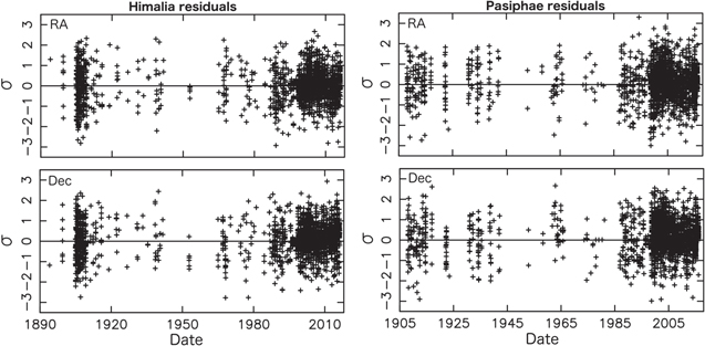
Figure 1. R.A. and decl. residuals for Himalia and Pasiphae in units of standard deviation.
Download figure:
Standard image High-resolution image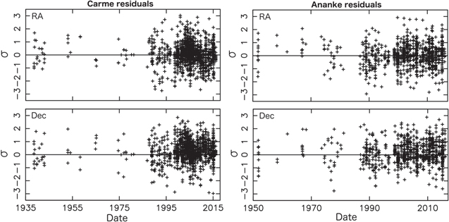
Figure 2. R.A. and decl. residuals for Carme and Ananke in units of standard deviation.
Download figure:
Standard image High-resolution imageFinally, we need to be careful when interpreting the residuals of fits to sparse data sets; such is the case for objects discovered in 2003. A number of these (2003 J2, 2003 J3, 2003 J10, 2003 J12, 2003 J15, 2003 J19) have less than two dozen measurements. Here, the rms of the residuals can be artificially small because the data points originate from few observing days and a single observer.
3.2. Epoch State Vectors
We list the epoch state vectors for Himalia, Carme, Ananke, and Pasiphae in Table 3, while the rest are shown in the supplementary material. These state vectors contain a large number of decimal places and can be used as the starting points in any future numerical integrations.
Table 3. Jupiter Barycentric State Vectors at 2010 January 1 TDB Referred to the ICRF
| Satellite | Position (km) | Velocity (km s−1) |
|---|---|---|
| Himalia | 4337825.635451561771 | 2.574863576913344332 |
| −6687812.237772628665 | 2.007997249599044132 | |
| −8448956.767690518871 | 0.302766297575448262 | |
| Pasiphae | 5944198.183062282391 | −1.679778381167610357 |
| −29431531.57849211991 | −0.090688057315072276 | |
| 3035462.130826421082 | 0.199057589881797420 | |
| Carme | −15704298.89821530133 | −1.226119239129557448 |
| −20269856.17753366753 | 0.9319800461038791894 | |
| −16022532.47981102765 | 0.5421491387984143095 | |
| Ananke | −4548260.877144060098 | 1.628456319227774340 |
| 26292247.96134518087 | 0.262476719060061925 | |
| −115726.6114112823998 | 0.842340511687675764 |
Note. This table is available in its entirety in machine-readable and Virtual Observatory (VO) forms in the online journal. A portion is shown here for guidance regarding its form and content.
Only a portion of this table is shown here to demonstrate its form and content. A Machine-readable versions of the full table are available.
Download table as: DataTypeset image
3.3. Planetary Perturbations
The Sun is the dominant perturber of the irregular Jovian satellites, but we also investigated the strength of the perturbations from Saturn, Uranus, and Neptune. In this part of the analysis, orbital fits were reconverged without a particular planet in the perturbers list and compared to the solution that had the full set of perturbers. The comparison of in-orbit, radial, and out-of-plane differences was done for 1900–2016. This is the length of time for which we have observations (at least for Himalia, Elara, and Pasiphae) and the influence of the perturbers could be detected.
The rms of the differences between the models that fit the data with and without Saturn is less than 1000 km for most satellites in the prograde group. The exception is Carpo, with rms ∼ 5000 km. Uranus has a very small influence on the progrades, a few tens of kilometers at most. The influence of Saturn is more significant for the retrograde satellites. The rms of the perturbations due to Saturn is tens of thousands of kilometers during the 1900–2016 period. The perturbations from Uranus are much less pronounced, up to a few hundred kilometers. These results are consistent with the preliminary conclusions in Jacobson (2000). For completeness, we also tested for the influence of Neptune, but the perturbations turned out to be on the order of several tens of kilometers, which is negligible when compared to the current data accuracy.
3.4. Mass of Himalia
Emelyanov (2005b) noted that Himalia and Elara had an ∼65 K km close encounter on 1949 July 15 and that Elara's orbital fit depends on the mass of Himalia. Himalia's mass determination was based on a subset of 280–326 measurements of Elara before and after the 1949 encounter. The obtained GM for Himalia was 0.28 ± 0.04 km3 s−2. This study also showed that observations of Lysithea did not improve Himalia's mass result despite one relatively close approach at 169 K km in 1954.
Our analysis had more measurements of Elara and Lysithea than Emelyanov (2005b). We used 129 R.A. and decl. measurements of Elara prior to 1949 and 1877 R.A. and 1876 decl. points between 1905 and 2016. There were 44 R.A. and decl. measurements of Lysithea prior to Himalia's encounter in 1954 and 772 astrometry points between 1938 and 2016. We obtained GM = 0.13 ± 0.02 km3 s−2, a formal 1σ error, which is about a factor of two smaller than the Emelyanov (2005b) mass.
We tested the robustness of our result by hard-wiring Himalia's mass to 0.28 km3 s−2 and 0.56 km3 s−2, or twice the Emelyanov (2005b) mass. For each case, we reconverged the orbital fit and calculated the rms of the residuals for Elara and, for completeness, Lysithea. We estimated a statistically significant change in the rms of the residuals as rms  (Hogg & Tanis 1993), where N is the number of degrees of freedom. This expression stems from the properties of χ2 distribution and the fact that it has a mean and variance of N and 2N, respectively. From here, the standard deviation of the reduced χ2 distribution is
  or
or  . This metric is acceptable assuming that the data have normally distributed errors with standard deviation of one and no cross-correlation.
Table 4 lists Himalia's masses and the corresponding reduced rms of the residuals for Elara and Lysithea. We found that the mass of Himalia needs to be almost twice as large as Emelyanov (2005b) before a statistically significant change occurs in the rms of the residuals for Elara. Despite using more measurements for Lysithea than Emelyanov (2005b), we also concluded that its orbit shows no significant sensitivity to Himalia's mass.
Table 4. Reduced rms of the Residuals of Elara and Lysithea as a Function of Himalia's Mass
| Himalia Mass | Density | Reduced rms Elara | Reduced rms Lysithea |
|---|---|---|---|
| (km3 s−2) | (g/cm3) | ( ) ) |
( ) ) |
| 0.13 | 1.55 | 0.9914σ | 1.0027σ |
| 0.28 | 2.26 | 1.0023σ | 1.0057σ |
| 0.56 | 6.52 | 1.0700σ | 1.0192σ |
Note. The number of points used in orbital fits is listed in Table 2.
Download table as: ASCIITypeset image
Figure 3 shows in-orbit, radial, and out-of-plane differences for Elara's orbit when we use our nominal mass for Himalia and the Emelyanov (2005b) mass for Himalia. The comparison is shown for the entire duration of Elara's data, 1935–2016. The largest difference of ∼2000 km is along the orbital track, and it is for the data taken just after the Himalia–Elara encounter in 1949. At Jupiter distance, 2000 km is ∼067, which is smaller than the observational errors for the data taken in the 1950s. This plot justifies our claim that the two mass values are statistically indistinguishable, but it also shows that the mass of Himalia cannot be that much larger than that given by Emelyanov (2005b) because the orbital differences would grow to a level that can be detected.
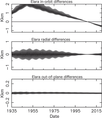
Figure 3. Differences in orbit of Elara due to a mass of Himalia of GM = 0.13 km3 s−2 or GM = 0.28 km3 s−2 (see Table 4).
Download figure:
Standard image High-resolution imageTable 4 also lists densities of Himalia. The density was calculated based on Cassini estimates (Porco et al. 2003) of the satellite's radius: 75 ± 10 km and 60 ± 10 km. We adopted an average radius of 67.5 km. Our nominal mass result suggests that Himalia is a low-density object. A factor of two increase in the Emelyanov (2005b) GM has an unlikely density of 6.5 g cm−3, and the residuals appear significantly worse. We thus conclude that Himalia's mass is in the 0.13–0.28 km3 s−2 range. We attempted to include other satellite masses in the orbital fits, but the data showed no sensitivity.
3.5. Accuracy of the Orbital Fits
The dominant sources of errors in orbital fits are star catalog errors and measurement errors. These errors are particularly relevant for the data taken before the CCD technology and modern data reduction techniques. All other components of the orbital fit have errors that are significantly smaller. The orbital model and the dynamical constants used in the model are well established. The uncertainties in the DE435 ephemerides of Jupiter are on the order of few tens of kilometers. The GMs of Jupiter and perturbing bodies are well known from the spacecraft data, so they are also not a significant factor in the fit accuracy.
We used a linear covariance mapping as described in Jacobson et al. (2012) to asses the orbital fit quality. Jacobson et al. (2012) evaluated the projection of the uncertainties on the plane of sky in R.A. and decl. on a particular date that was either three or 10 orbital periods beyond 2012 January. This method produced a result that is dependent on the orbital geometry at a particular date. The R.A. and decl. uncertainties on the plane of sky can be small for a short period of time and grow orders of magnitude for other dates.
In order to account for the uncertainties changing with time, we mapped the covariance over 2 yr, 2009–2011 January, 2019–2021 January, and 2029–2031 January. Two years is an approximate duration of orbital periods for most Jovian irregulars. We examine the rms of the uncertainties in the in-orbit, radial, and out-of-plane directions during these times. For completeness, we also project the uncertainties on the plane of sky and evaluate the maximum plane-of-sky (combined R.A. and decl.) uncertainty. These maximum values should provide good constraints on the search region if further observations are planned. Furthermore, we get a quick assessment of the orbital status, i.e., the satellite position is known, recoverable, or lost. We consider anything with a plane-of-sky uncertainty larger than 1000'' to be lost. For comparison, Jupiter's average Hill sphere is 14,000''.
Table 5 list results for Himalia, Pasiphae, Ananke, and Carme, while other satellites are listed in the supplementary material. We note that in-orbit (or transverse) uncertainties grow as a result of uncertainties in the mean motion. We plot the growth of the plane-of-sky uncertainties from 2010 to 2030 for Himalia, Pasiphae, Ananke, and Carme in Figure 4. The general secular growth for the four satellites in Figure 4 is below 70 mas until at least 2030, which means that these satellites are in no danger of being lost.
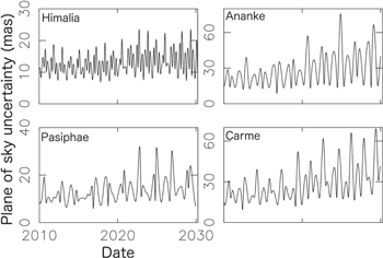
Figure 4. Plane-of-sky uncertainties for Himalia, Pasiphae, Ananke, and Carme from 2010 to 2030.
Download figure:
Standard image High-resolution imageTable 5. Orbital Uncertainties in the Plane-of-sky (summed R.A. and decl.), In-orbit, Radial, and Out-of-plane Directions
| Satellite | Year | Plane-of-sky | In-orbit | Radial | Out-of-plane |
|---|---|---|---|---|---|
| (arcsec) | (km) | (km) | (km) | ||
| Himalia | 2010 | 0.02 | 46 | 18 | 27 |
| 2020 | 0.02 | 56 | 20 | 28 | |
| 2030 | 0.02 | 68 | 20 | 28 | |
| Pasiphae | 2010 | 0.02 | 37 | 15 | 26 |
| 2020 | 0.02 | 57 | 24 | 24 | |
| 2030 | 0.02 | 73 | 29 | 25 | |
| Carme | 2010 | 0.03 | 72 | 28 | 45 |
| 2020 | 0.06 | 130 | 37 | 43 | |
| 2030 | 0.07 | 210 | 46 | 43 | |
| Ananke | 2010 | 0.03 | 78 | 30 | 42 |
| 2020 | 0.05 | 130 | 43 | 40 | |
| 2030 | 0.07 | 180 | 53 | 39 | |
Note. The uncertainties are calculated for 2 yr intervals centered on 2010, 2020, and 2030 January 1. The plane-of-sky uncertainty is the maximum uncertainty during the 2 yr time interval, while the in-orbit, radial, and out-of-plane values are the rms of the uncertainties. This table is available in its entirety in machine-readable and Virtual Observatory (VO) forms in the online journal. A portion is shown here for guidance regarding its form and content.
Only a portion of this table is shown here to demonstrate its form and content. A Machine-readable versions of the full table are available.
Download table as: DataTypeset image
There are currently 11 irregular satellites, all with provisional IAU designations, that have observations spanning less than 1 yr. Ten of these satellites have not been observed since 2003, which means that they are likely lost. Likewise, one of the satellites discovered in 2011, 2011 J1, has the plane-of-sky uncertainty of hundreds of arcseconds and is on the verge of being lost. Figure 2 in Jacobson et al. (2012) shows that even a satellite with few hundred arcsecond plane-of-sky uncertainty could be recovered with a telescope that has large enough field of view. The observations also need to be carefully planned so that the satellite is observed when the uncertainties have favorable orbital geometry projection.
3.6. Mean Orbital Elements
Results of orbital integration can be expressed in terms of planetocentric mean orbital elements (Brozović & Jacobson 2009; Brozović et al. 2011; Jacobson et al. 2012). We take the state vectors listed in Table 3 and propagate them backward and forward in time from 1600 February to 2599 September using the same set of perturbers as described in Section 2. This produces positions of the satellites over a period of 1000 yr of orbital integration. These "measurements" are compared to the positions from an analytical model, a precessing ellipse. The initial elements and rates of the model are refined via the least-squares procedure until the fit shows no further improvement. The ellipse captures the constant and secular properties of the integrated orbit, and the differences that remain are due to periodic perturbations. The mean elements listed in Table 6 are a descriptive representation of the integrated orbits; hence, there are no uncertainties associated with the elements. We have already discussed the orbital uncertainties for the integrated orbits in Section 3.5.
Table 6. Planetocentric Mean Orbital Elements in Ecliptic Coordinates for 59 Irregular Jovian Satellites
| Satellite | a | e | i | λ | ϖ | Ω | d λ/dt | Pλ | d ϖ/dt | d Ω/dt | ν | Class |
|---|---|---|---|---|---|---|---|---|---|---|---|---|
| (km) | (deg) | (deg) | (deg) | (deg) | (deg/day) | (days) | (deg yr−1) | (deg yr−1) | ||||
| Carpo | 17056600 | 0.432 | 51.62 | 120.21 | 109.05 | 18.68 | 0.7890 | 456.28 | −3.1915 | −3.1910 | −1.00 | LK, MSC |
| Themisto | 7503900 | 0.243 | 42.98 | 36.94 | 47.89 | 185.47 | 2.7688 | 130.02 | −0.1567 | −0.6813 | −0.23 | RC, MSC |
| Dia | 12297500 | 0.232 | 28.63 | 104.68 | 123.76 | 279.61 | 1.2940 | 278.21 | 1.5737 | −1.4881 | 1.06 | DC, Non-MS |
| Elara | 11740300 | 0.211 | 27.94 | 253.50 | 272.05 | 101.94 | 1.3865 | 259.64 | 1.4540 | −1.3569 | 1.07 | DC, Non-MS |
| Leda | 11164400 | 0.162 | 27.88 | 57.39 | 141.52 | 207.26 | 1.4942 | 240.93 | 1.2941 | −1.1923 | 1.09 | DC, Non-MS |
| Himalia | 11460200 | 0.159 | 28.61 | 311.38 | 49.56 | 52.49 | 1.4368 | 250.56 | 1.3524 | −1.2305 | 1.10 | DC, Non-MS |
| Lysithea | 11717000 | 0.116 | 27.66 | 59.08 | 70.12 | 353.00 | 1.3889 | 259.20 | 1.5115 | −1.2327 | 1.23 | DC, Non-MS |
| Euporie | 19336200 | 0.144 | 145.74 | 328.05 | 3.95 | 85.96 | 0.6537 | 550.69 | −2.5805 | 2.5816 | −1.00 | LK, MSC |
| 2003 J18 | 20491400 | 0.090 | 146.20 | 213.74 | 312.64 | 183.76 | 0.6019 | 598.14 | −2.0218 | 2.7495 | −0.74 | RC, MSC |
| 2003 J15 | 22565200 | 0.191 | 146.90 | 307.61 | 126.89 | 267.61 | 0.5219 | 689.79 | −1.5020 | 3.4526 | −0.44 | RC, MSC |
| 2003 J3 | 20210000 | 0.197 | 147.63 | 238.84 | 185.17 | 262.26 | 0.6166 | 583.84 | −0.9533 | 2.9166 | −0.33 | RC, MSC |
| 2003 J23 | 23601700 | 0.276 | 146.51 | 350.86 | 202.01 | 81.93 | 0.4900 | 734.64 | −1.1040 | 3.8750 | −0.28 | RC, MSC |
| Callirrhoe | 24098900 | 0.280 | 147.08 | 141.83 | 90.35 | 323.54 | 0.4744 | 758.82 | −1.0448 | 4.0435 | −0.26 | RC, MSC |
| Thyone | 21197200 | 0.231 | 148.59 | 39.56 | 215.94 | 265.48 | 0.5740 | 627.19 | −0.8059 | 3.2452 | −0.25 | RC, MSC |
| Orthosie | 21158200 | 0.281 | 146.00 | 151.68 | 346.67 | 255.43 | 0.5782 | 622.58 | −0.8189 | 3.3478 | −0.24 | RC, MSC |
| Ananke | 21253700 | 0.233 | 148.69 | 261.30 | 71.96 | 48.66 | 0.5716 | 629.80 | −0.7851 | 3.2692 | −0.24 | RC, MSC |
| Harpalyke | 21106100 | 0.230 | 148.76 | 270.42 | 96.88 | 62.09 | 0.5776 | 623.32 | −0.7787 | 3.2248 | −0.24 | RC, MSC |
| Mneme | 21033000 | 0.226 | 148.58 | 244.87 | 19.32 | 45.54 | 0.5806 | 620.05 | −0.7755 | 3.2069 | −0.24 | RC, MSC |
| 2003 J16 | 21089700 | 0.228 | 148.74 | 299.80 | 33.18 | 47.95 | 0.5780 | 622.89 | −0.7717 | 3.2381 | −0.24 | RC, MSC |
| Iocaste | 21272000 | 0.215 | 149.41 | 290.93 | 147.42 | 302.00 | 0.5700 | 631.60 | −0.7685 | 3.2380 | −0.24 | RC, MSC |
| 2010 J2 | 21004200 | 0.227 | 148.67 | 289.62 | 4.89 | 37.85 | 0.5817 | 618.85 | −0.7562 | 3.2043 | −0.24 | RC, MSC |
| Praxidike | 21147700 | 0.227 | 148.88 | 330.19 | 262.38 | 313.35 | 0.5756 | 625.39 | −0.7518 | 3.2384 | −0.23 | RC, MSC |
| Euanthe | 21039000 | 0.232 | 148.92 | 359.01 | 59.02 | 286.53 | 0.5802 | 620.45 | −0.7316 | 3.2227 | −0.23 | RC, MSC |
| Kore | 24481800 | 0.331 | 145.17 | 110.98 | 175.31 | 355.98 | 0.4634 | 776.84 | −0.9408 | 4.2620 | −0.22 | RC, MSC |
| Hermippe | 21297100 | 0.210 | 150.74 | 16.85 | 324.20 | 2.94 | 0.5679 | 633.91 | −0.6246 | 3.2539 | −0.19 | RC, MSC |
| Eurydome | 23146200 | 0.275 | 150.27 | 242.20 | 274.84 | 341.06 | 0.5019 | 717.31 | −0.6322 | 3.8586 | −0.16 | RC, MSC |
| Thelxinoe | 21159700 | 0.220 | 151.39 | 345.22 | 138.19 | 202.57 | 0.5732 | 628.03 | −0.5035 | 3.2604 | −0.15 | RC, MSC |
| Sponde | 23790100 | 0.311 | 151.00 | 76.94 | 300.85 | 157.74 | 0.4811 | 748.32 | −0.4671 | 4.1375 | −0.11 | RC, MSC |
| Helike | 21065500 | 0.150 | 154.84 | 193.06 | 206.56 | 121.20 | 0.5748 | 626.33 | −0.3180 | 3.1438 | −0.10 | RC, MSC |
| 2003 J4 | 23928700 | 0.362 | 149.59 | 220.01 | 14.80 | 222.53 | 0.4767 | 755.25 | −0.3469 | 4.3393 | −0.08 | RC, MSC |
| Autonoe | 24037200 | 0.315 | 152.37 | 212.09 | 138.62 | 315.18 | 0.4731 | 761.01 | −0.3363 | 4.2355 | −0.08 | RC, MSC |
| Sinope | 23942000 | 0.255 | 158.19 | 143.59 | 44.73 | 350.39 | 0.4744 | 758.89 | −0.0614 | 4.1189 | −0.01 | ∼SR, RC |
| Hegemone | 23574700 | 0.344 | 154.16 | 92.76 | 237.85 | 1.32 | 0.4866 | 739.82 | −0.0392 | 4.2417 | −0.01 | ∼SR, RC |
| 2011 J2 | 23124300 | 0.349 | 153.60 | 201.52 | 244.91 | 66.24 | 0.5011 | 718.40 | −0.0370 | 4.1380 | −0.01 | ∼SR, RC |
| Cyllene | 23799600 | 0.415 | 150.33 | 11.98 | 294.54 | 297.79 | 0.4787 | 751.98 | −0.0273 | 4.5165 | −0.01 | ∼SR, RC |
| Pasiphae | 23629100 | 0.406 | 151.41 | 103.27 | 214.99 | 358.58 | 0.4841 | 743.61 | −0.0015 | 4.4351 | 0.00 | SR |
| Magaclite | 23813900 | 0.416 | 152.78 | 90.32 | 9.69 | 326.02 | 0.4782 | 752.88 | 0.1381 | 4.5435 | 0.03 | DC, MSC |
| 2003 J2 | 28348600 | 0.410 | 157.29 | 319.56 | 182.90 | 42.03 | 0.3671 | 980.59 | 0.2482 | 5.7262 | 0.04 | DC, MSC |
| Carme | 23400500 | 0.255 | 164.99 | 136.19 | 275.26 | 155.62 | 0.4904 | 734.17 | 0.3696 | 4.0761 | 0.09 | DC, MSC |
| Kalyke | 23564600 | 0.247 | 165.12 | 43.02 | 178.59 | 84.93 | 0.4851 | 742.04 | 0.3516 | 4.1063 | 0.09 | DC, MSC |
| 2010 J1 | 23448500 | 0.249 | 165.10 | 52.47 | 269.94 | 323.63 | 0.4888 | 736.50 | 0.3588 | 4.0755 | 0.09 | DC, MSC |
| Arche | 23352000 | 0.249 | 165.01 | 228.94 | 196.08 | 19.79 | 0.4919 | 731.90 | 0.3656 | 4.0572 | 0.09 | DC, MSC |
| Herse | 23407900 | 0.254 | 164.96 | 166.65 | 38.26 | 336.49 | 0.4901 | 734.52 | 0.3669 | 4.0787 | 0.09 | DC, MSC |
| 2003 J5 | 23424100 | 0.251 | 165.24 | 235.57 | 277.53 | 216.81 | 0.4895 | 735.40 | 0.3716 | 4.0862 | 0.09 | DC, MSC |
| 2003 J19 | 23545900 | 0.256 | 165.13 | 347.26 | 152.89 | 69.23 | 0.4858 | 741.03 | 0.3720 | 4.1195 | 0.09 | DC, MSC |
| Kallichore | 23276300 | 0.251 | 165.10 | 41.28 | 343.26 | 70.72 | 0.4943 | 728.24 | 0.3762 | 4.0378 | 0.09 | DC, MSC |
| Taygete | 23362900 | 0.252 | 165.25 | 16.72 | 290.22 | 345.76 | 0.4915 | 732.41 | 0.3783 | 4.0637 | 0.09 | DC, MSC |
| 2011 J1 | 23444400 | 0.253 | 165.34 | 22.78 | 144.62 | 290.55 | 0.4889 | 736.33 | 0.3792 | 4.1078 | 0.09 | DC, MSC |
| Isonoe | 23231200 | 0.247 | 165.25 | 121.61 | 349.72 | 171.18 | 0.4957 | 726.26 | 0.3795 | 4.0212 | 0.09 | DC, MSC |
| Kale | 23305800 | 0.260 | 164.94 | 199.36 | 347.91 | 100.82 | 0.4934 | 729.61 | 0.3845 | 4.0647 | 0.09 | DC, MSC |
| Chaldene | 23180600 | 0.250 | 165.16 | 34.17 | 113.51 | 174.46 | 0.4974 | 723.73 | 0.3873 | 4.0213 | 0.10 | DC, MSC |
| Erinome | 23285900 | 0.266 | 164.91 | 325.12 | 56.73 | 358.26 | 0.4942 | 728.49 | 0.3957 | 4.0758 | 0.10 | DC, MSC |
| Aitne | 23316700 | 0.263 | 165.05 | 196.91 | 94.70 | 49.51 | 0.4931 | 730.12 | 0.3976 | 4.0822 | 0.10 | DC, MSC |
| 2003 J9 | 23334700 | 0.266 | 165.03 | 233.88 | 253.10 | 84.99 | 0.4925 | 730.93 | 0.3992 | 4.0941 | 0.10 | DC, MSC |
| Eukelade | 23322700 | 0.262 | 165.26 | 321.63 | 120.16 | 234.40 | 0.4929 | 730.33 | 0.4030 | 4.0836 | 0.10 | DC, MSC |
| Pasithee | 23091500 | 0.268 | 165.12 | 147.48 | 268.41 | 8.07 | 0.5004 | 719.47 | 0.4207 | 4.0336 | 0.10 | DC, MSC |
| Aoede | 23974100 | 0.432 | 158.27 | 11.20 | 251.54 | 220.26 | 0.4728 | 761.40 | 0.5186 | 4.6854 | 0.11 | DC, MSC |
| 2003 J12 | 17818600 | 0.491 | 151.08 | 152.07 | 311.60 | 96.85 | 0.7352 | 489.67 | 0.3863 | 3.3079 | 0.12 | DC, MSC |
| 2003 J10 | 22862300 | 0.475 | 168.79 | 309.54 | 28.30 | 210.28 | 0.5003 | 719.55 | 0.9299 | 4.4810 | 0.21 | DC, MSC |
| Jupiter | 777634000 | 0.045 | 16.27 | 337.66 | 16.27 | 102.26 | 0.0831 | 4332.59 | 0.0017 | 0.0013 | ... | ... |
Note. The epoch for the orbital elements is 2010 January 1 TDB. The horizontal line divides the satellites into prograde and retrograde groups. Listed are semimajor axis, a, eccentricity, e, inclination, i, mean longitude, λ, longitude of periapsis, ϖ, longitude of the ascending node, Ω, mean longitude rate, dλ/dt, orbital period, Pλ, rate of apsidal precession, dϖ/dt, rate of nodal precession, dΩ/dt, ratio of apsidal and nodal precession rates  for prograde and
  for retrograde, and a classification based on a value of ν. The categories are the same as in Ćuk & Burns (2004): Lidov–Kozai librators, LK, reverse circulators, RC, direct circulators, DC, non-main-sequence objects, Non-MS, main-sequence circulators, MSC, and secular resonators, SR. We also list the heliocentric mean orbital elements for Jupiter.
Download table as: ASCIITypeset image
We use a ratio of the apsidal and nodal precession rates, ν, to classify the orbits similarly to Ćuk & Burns (2004). We define the longitude of periapsis as ϖ = Ω + ω for prograde orbits and ϖ = Ω − ω for retrograde orbits. Here, Ω is longitude of the ascending node and ω is argument of periapsis. If the argument of periapsis is circulating slower than the node, the object is marked as a reverse circulator (RC). If the argument of periapsis is circulating faster than the node, the object is marked as a direct circulator (DC). The satellites that are the Lidov–Kozai librators (Lidov 1962; Kozai 1962) have ν = −1. The objects that are close to the secular resonance with Jupiter have their rates of apsidal precession matched to that of Jupiter,  , and consequently, they have ν = 0. Ćuk & Burns (2004) also classified objects as main-sequence circulators (MSC) or non-main-sequence (non-MS) residents with respect to how close they are to the secular resonance with Jupiter. The MSC objects are direct circulators with ν < 0.2, or reverse circulators with orbital parameters between the Lidov–Kozai and secular resonances. The non-MS objects have ν ≥ 0.2.
Table 6 shows that all objects considered to be part of Himalia's prograde group, that is, Himalia, Elara, Lysithea, Leda, and Dia, are direct circulators. Themisto and Carpo clearly do not belong to this group as one is a reverse circulator and the other is in the Lidov–Kozai resonance. Themisto orbits Jupiter at 75 M km, and its orbital period is only 130 days.
The retrograde group is about equally split into reverse and direct circulators, except Euporie, which is another Lidov–Kozai resonator, and Pasiphae, which is in secular resonance with Jupiter (Whipple & Shelus 1993). According to the present orbital solution, 2003 J18 appears to reside close to the Lidov–Kozai region. In addition, there are some interesting outliers, such as 2003 J2 and 2003 J12, which have orbital periods of 981 and 490 days, respectively, while all other retrogrades have periods from 550 to 760 days.
We used JPL planetary ephemeris DE431 (Folkner et al. 2014), which spans 17,000 yr (−8002 December to 9001 April), to calculate the heliocentric mean orbital elements in ecliptic coordinates for Jupiter and to obtain the nodal and apsidal precession rates (also listed in Table 6). A direct comparison of the apsidal precession rates of Jupiter with those of Pasiphae, Cylene, 2011 J2, Hegemone, and Sinope shows that Pasiphae is in secular resonance, but that the others are not too far from the resonance themselves.
Figure 5 is a summary of the spatial distribution of the Jovian irregulars in terms of  and
and  . The radial distance from the origin is expressed in the units of Hill radii (0.36 au for Jupiter). Almost all satellites show large pericenter-to-apocenter differences in their orbits. Eighteen of the retrograde satellites form a tight group, with Carme as the largest member (panel (a) in Figure 5). Another nine retrogrades (Iocaste included) form another cluster, with Ananke as the largest member (panel (b) in Figure 5). The third obvious cluster is Himalia's prograde group, with Himalia, Leda, Elara, Lysithea, and Dia as the members (panel (c) in Figure 5). The Pasiphae cluster (Pasiphae, Megaclite, 2003 J4, and Cyllene) uncovered by Beaugé & Nesvorný (2007) does not stand out as much as the other ones, and a more sophisticated analysis, beyond the scope of this paper, would be required to attempt a formal clustering.
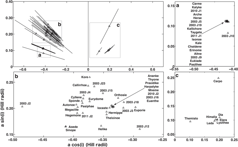
Figure 5. Spatial distribution for the irregular Jovian satellites is shown in the top left panel. The other panels show close-up views of this plot so that the names of the satellites are visible. The lines represent the pericenter-to-apocenter distances, a(1 − e) to a(1 + e).
Download figure:
Standard image High-resolution image4. Concluding Remarks
Our analysis is an extension of Jacobson (2000) and Jacobson et al. (2012) orbital fits for the irregular Jovian satellites. We used numerically integrated orbits with a full set of perturbers and a weighted least-squares method to fit the Earth-based astrometric observations, as well as a handful of the New Horizons spacecraft astrometric measurements of Himalia and Callirrhoe. The Sun has a major influence on the orbital fits and to some extent Saturn. Saturn perturbs the retrograde satellites more than the progrades.
The astrometric data set is more than a century long for Himalia, Elara, Pasiphae, and Sinope. Other satellites have data sets that range from several decades to less than a year. Out of 59 satellites, 11 are likely lost. The long data arcs for Himalia and Elara allowed for Himalia's mass determination to within about a factor of two, GM = 0.13–0.28 km3 s−2. We confirmed a finding by Emelyanov (2005b) that Himalia's mass has very little influence on the orbit of Lysithea and that the mass determination was mitigated by Himalia's and Elara's encounter at 65 K km in 1949. We investigated a possibility of mass determination for other satellites given the size and length of the data set, but no mass sensitivity beyond Himalia's was found.
We calculated mean orbital elements for 1000 yr of integrated orbits. We have shown that Jovian irregulars represent a diverse dynamical system, with Carpo and Euporie as examples of objects that are caught in Lindov–Kozai resonance. We have also confirmed that Pasiphae is in a secular resonance with Jupiter. Cyllene, 2011 J2, Hegemone, and Sinope also appear to be close to the resonance.
We decided not to go beyond the visual clustering of the satellites into groups based on Figure 5 given that the Beaugé & Nesvorný (2007) analysis of the Jovian irregulars covered 53 out of 59 satellites reported here. Their study assumed that the irregular satellites are collisional products, and they used proper elements and hierarchical clustering to identify satellite families. Beaugé & Nesvorný (2007) results showed that only about 60% of the retrograde satellites can be associated with Carme, Ananke, and Pasiphae, while other irregulars do not show strong clustering.
The solution discussed in this article is our latest and most complete determination of the orbits. It is posted as JUP340 on JPL's Horizons online solar system data and ephemeris computation service (Giorgini et al. 1996) and NASA's Navigation and Ancillary Information Facility (Acton 1996).
The research described here was carried out at the Jet Propulsion Laboratory, California Institute of Technology, under contract with the National Aeronautics and Space Administration. The authors would like to thank all of the astronomers who contributed with their measurements to these orbital calculations. The authors also thank the anonymous reviewer, whose comments helped improve this paper.
Appendix: Osculating Elements
Osculating orbital elements are calculated by converting the state vectors from integrated orbits into Keplerian orbital elements that only assume two-body interaction. The osculating elements do not include any of the J2 effects, but they still provide a sense of how the orbit changes over the long time intervals.
Plots of osculating eccentricity, inclination, and argument of periapsis quickly reveal the typical behavior of an object caught in the Lindov–Kozai resonance. Two such objects, Carpo and Euporie, are shown in Figure 6. Both of these satellites have their respective arguments librating about 90°, while the eccentricity and inclination endure coupled oscillations. For Carpo, the eccentricity varies between 0.19 and 0.69, while the inclination changes from 44° to 59°. The orbit of Euporie is much less eccentric, and over 1000 yr the eccentricity varies between 0.07 and 0.27, while the inclination changes from 142° to 149°. We list the minimum and maximum values for osculating a, e, and i for all irregular Jovian satellites over a 1000 yr interval in Table 7.

Figure 6. Carpo and Euporie are irregular Jovian satellites caught in the Lidov–Kozai resonance. The resonance is evident in the oscillating argument of periapsis.
Download figure:
Standard image High-resolution image
Table 7. Minimum and Maximum Values of Osculating Orbital Elements, and Their Averages over 1000 yr
| Satellite | Min aosc | Mean aosc | Max aosc | Min eosc | Mean eosc | Max eosc | Min iosc | Mean iosc | Max iosc |
|---|---|---|---|---|---|---|---|---|---|
| (km) | (km) | (km) | (deg) | (deg) | (deg) | ||||
| Carpo | 16525900 | 17043100 | 17622300 | 0.194 | 0.425 | 0.691 | 43.8 | 53.1 | 59.2 |
| Themisto | 7377200 | 7398400 | 7417800 | 0.075 | 0.254 | 0.463 | 38.7 | 44.3 | 48.4 |
| Dia | 12131000 | 12260400 | 12414500 | 0.164 | 0.233 | 0.305 | 25.9 | 28.9 | 31.7 |
| Elara | 11608200 | 11712300 | 11837500 | 0.152 | 0.212 | 0.275 | 25.5 | 28.1 | 30.8 |
| Leda | 11061100 | 11146400 | 11243300 | 0.116 | 0.163 | 0.212 | 25.7 | 28.0 | 30.4 |
| Himalia | 11344400 | 11440600 | 11543000 | 0.111 | 0.160 | 0.209 | 26.2 | 28.7 | 30.9 |
| Lysithea | 11602900 | 11700800 | 11804900 | 0.078 | 0.117 | 0.156 | 25.5 | 27.7 | 29.7 |
| Euporie | 18729800 | 19265900 | 19815200 | 0.066 | 0.148 | 0.267 | 141.7 | 145.5 | 148.8 |
| 2003 J18 | 19673600 | 20336700 | 21011800 | 0.000 | 0.104 | 0.305 | 141.5 | 145.6 | 149.7 |
| 2003 J15 | 21384500 | 22337800 | 23449800 | 0.012 | 0.205 | 0.470 | 139.7 | 145.5 | 151.3 |
| 2003 J3 | 19381000 | 20017100 | 20741300 | 0.049 | 0.209 | 0.411 | 141.7 | 146.8 | 151.7 |
| 2003 J23 | 22191200 | 23301300 | 24734400 | 0.051 | 0.290 | 0.590 | 136.7 | 144.5 | 151.7 |
| Callirrhoe | 22581000 | 23794400 | 25341300 | 0.057 | 0.293 | 0.600 | 137.1 | 145.1 | 152.5 |
| Thyone | 20215300 | 20977600 | 21880500 | 0.067 | 0.242 | 0.458 | 142.2 | 147.6 | 153.0 |
| Orthosie | 20128100 | 20901900 | 21819900 | 0.076 | 0.292 | 0.567 | 136.9 | 144.2 | 150.9 |
| Ananke | 20262900 | 21034500 | 21970100 | 0.068 | 0.245 | 0.460 | 142.0 | 147.7 | 153.1 |
| Harpalyke | 20148300 | 20891600 | 21786000 | 0.073 | 0.241 | 0.450 | 142.0 | 147.8 | 153.1 |
| Mneme | 20080500 | 20819600 | 21681800 | 0.067 | 0.237 | 0.454 | 142.1 | 147.7 | 153.0 |
| 2003 J16 | 20129000 | 20881900 | 21776700 | 0.069 | 0.239 | 0.455 | 141.9 | 147.8 | 152.9 |
| Iocaste | 20290500 | 21066700 | 21969500 | 0.066 | 0.226 | 0.427 | 143.0 | 148.6 | 153.4 |
| 2010 J2 | 20058100 | 20792800 | 21674800 | 0.067 | 0.238 | 0.448 | 142.1 | 147.8 | 153.1 |
| Praxidike | 20177400 | 20935500 | 21859700 | 0.071 | 0.238 | 0.450 | 142.2 | 148.0 | 153.2 |
| Euanthe | 20084600 | 20827400 | 21726000 | 0.074 | 0.243 | 0.455 | 142.2 | 148.0 | 153.2 |
| Kore | 22888000 | 24208300 | 25961400 | 0.061 | 0.340 | 0.693 | 132.5 | 141.9 | 151.4 |
| Hermippe | 20338600 | 21108000 | 22026400 | 0.069 | 0.219 | 0.406 | 144.8 | 150.1 | 154.6 |
| Eurydome | 21852500 | 22899200 | 24248400 | 0.086 | 0.287 | 0.525 | 142.1 | 148.9 | 154.9 |
| Thelxinoe | 20221100 | 20977200 | 21884100 | 0.081 | 0.229 | 0.412 | 145.4 | 150.7 | 155.3 |
| Sponde | 22403600 | 23543800 | 25132800 | 0.116 | 0.322 | 0.576 | 141.5 | 149.3 | 155.7 |
| Helike | 20186100 | 20915900 | 21756100 | 0.052 | 0.156 | 0.289 | 150.5 | 154.5 | 157.7 |
| 2003 J4 | 22478900 | 23715200 | 25395000 | 0.130 | 0.371 | 0.657 | 137.8 | 146.9 | 155.0 |
| Autonoe | 22568600 | 23790700 | 25385300 | 0.117 | 0.326 | 0.574 | 143.1 | 150.7 | 157.1 |
| Sinope | 22519500 | 23685400 | 25257600 | 0.097 | 0.265 | 0.464 | 151.9 | 157.4 | 161.5 |
| Hegemone | 22219500 | 23347500 | 24748500 | 0.151 | 0.353 | 0.590 | 144.1 | 152.4 | 158.2 |
| 2011 J2 | 21875800 | 22909400 | 24240500 | 0.160 | 0.358 | 0.600 | 143.5 | 151.8 | 157.6 |
| Cyllene | 22407100 | 23653900 | 25386100 | 0.171 | 0.420 | 0.700 | 136.6 | 146.8 | 155.3 |
| Pasiphae | 22276600 | 23467500 | 24984100 | 0.174 | 0.411 | 0.675 | 138.9 | 148.3 | 156.2 |
| Megaclite | 22385500 | 23646400 | 25451600 | 0.179 | 0.421 | 0.686 | 139.9 | 149.7 | 157.5 |
| 2003 J2 | 25790500 | 28041100 | 31603300 | 0.133 | 0.423 | 0.701 | 143.9 | 154.5 | 161.7 |
| Carme | 22083200 | 23144800 | 24590900 | 0.115 | 0.263 | 0.420 | 160.2 | 164.5 | 167.7 |
| Kalyke | 22216300 | 23302800 | 24778000 | 0.105 | 0.255 | 0.411 | 160.6 | 164.7 | 167.8 |
| 2010 J1 | 22121200 | 23190500 | 24619800 | 0.110 | 0.257 | 0.414 | 160.4 | 164.6 | 167.8 |
| Arche | 22034400 | 23098000 | 24516100 | 0.112 | 0.257 | 0.415 | 160.2 | 164.5 | 167.7 |
| Herse | 22099700 | 23152300 | 24589500 | 0.111 | 0.262 | 0.418 | 160.0 | 164.5 | 167.7 |
| 2003 J5 | 22109700 | 23168000 | 24606100 | 0.110 | 0.259 | 0.417 | 160.5 | 164.8 | 168.0 |
| 2003 J19 | 22210500 | 23283600 | 24758100 | 0.116 | 0.264 | 0.424 | 160.3 | 164.6 | 167.9 |
| Kallichore | 21988600 | 23022900 | 24421600 | 0.113 | 0.259 | 0.413 | 160.8 | 164.6 | 167.8 |
| Taygete | 22050900 | 23107400 | 24498800 | 0.114 | 0.260 | 0.416 | 160.5 | 164.8 | 167.9 |
| 2011 J1 | 22107100 | 23187500 | 24639800 | 0.113 | 0.261 | 0.422 | 160.4 | 164.8 | 168.0 |
| Isonoe | 21959000 | 22981400 | 24362400 | 0.112 | 0.255 | 0.408 | 161.0 | 164.8 | 167.9 |
| Kale | 22009800 | 23052800 | 24497200 | 0.115 | 0.268 | 0.422 | 160.1 | 164.4 | 167.7 |
| Chaldene | 21903800 | 22930800 | 24295700 | 0.112 | 0.258 | 0.413 | 160.6 | 164.7 | 167.8 |
| Erinome | 21968000 | 23031500 | 24453600 | 0.124 | 0.273 | 0.426 | 159.8 | 164.4 | 167.7 |
| Aitne | 22014100 | 23063900 | 24493100 | 0.120 | 0.271 | 0.429 | 160.5 | 164.5 | 167.8 |
| 2003 J9 | 22026200 | 23080600 | 24474500 | 0.126 | 0.274 | 0.430 | 160.4 | 164.5 | 167.9 |
| Eukelade | 22006300 | 23067300 | 24491600 | 0.123 | 0.270 | 0.425 | 160.6 | 164.8 | 168.0 |
| Pasithee | 21839200 | 22846700 | 24230800 | 0.124 | 0.276 | 0.433 | 160.3 | 164.6 | 167.9 |
| Aoede | 22477300 | 23777700 | 25648800 | 0.227 | 0.438 | 0.651 | 146.4 | 155.8 | 162.5 |
| 2003 J12 | 17362700 | 17833400 | 18461800 | 0.290 | 0.485 | 0.699 | 137.1 | 146.8 | 156.2 |
| 2003 J10 | 21748000 | 22884600 | 24557000 | 0.276 | 0.475 | 0.657 | 156.1 | 163.2 | 168.5 |
Download table as: ASCIITypeset image