


ABSTRACT
The hemispheric preference for negative/positive helicity to occur in the northern/southern solar hemisphere provides clues to the causes of twisted, flaring magnetic fields. Previous studies on the hemisphere rule may have been affected by seeing from atmospheric turbulence. Using Hinode/SOT-SP data spanning 2006–2013, we studied the effects of two spatial smoothing tests that imitate atmospheric seeing: noise reduction by ignoring pixel values weaker than the estimated noise threshold, and Gaussian spatial smoothing. We studied in detail the effects of atmospheric seeing on the helicity distributions across various field strengths for active regions (ARs) NOAA 11158 and NOAA 11243, in addition to studying the average helicities of 179 ARs with and without smoothing. We found that, rather than changing trends in the helicity distributions, spatial smoothing modified existing trends by reducing random noise and by regressing outliers toward the mean, or removing them altogether. Furthermore, the average helicity parameter values of the 179 ARs did not conform to the hemisphere rule: independent of smoothing, the weak-vertical-field values tended to be negative in both hemispheres, and the strong-vertical-field values tended to be positive, especially in the south. We conclude that spatial smoothing does not significantly affect the overall statistics for space-based data, and thus seeing from atmospheric turbulence seems not to have significantly affected previous studies' ground-based results on the hemisphere rule.
Export citation and abstract BibTeX RIS
1. INTRODUCTION
Magnetic helicity describes the internal complexity of magnetic flux tubes in a solar active region (AR; Berger 1984). While magnetic helicity is difficult to measure directly, solar magnetic helicity patterns can be studied using well-known parameters that are simpler to calculate, such as electric current helicity,

which can be calculated pixel-by-pixel:

where Bz is the vertical magnetic field component and Jz ≡ (curl  )z, or through α, the twist per unit length along field lines. It is useful to distinguish between global and local components of α, in order to capture both large-scale (hemispherical) and smaller (local) trends in helicity (Pevtsov et al. 1994). Local twist, αloc, can be derived pixel-by-pixel:

The helicity of the solar field is observed to obey a hemispheric sign rule, where helicity is predominantly positive in the southern hemisphere and negative in the northern (Seehafer 1990). Pevtsov et al. (1995) confirmed the hemisphere rule using αave values derived from best-fitting linear force-free field models to vector magnetograms, optimizing over entire ARs. They also found a latitudinal variation in helicity, with αave being the largest around 15°–25° latitude. The helicities of fields with strong and weak vertical components Bz (found around the umbrae and penumbrae of sunspots, respectively) show distinct hemispherical trends. Zhang (2006) found that both αave and Hc followed the hemisphere rule for weak-Bz fields, but had signs opposite to the hemisphere rule's prediction for strong-Bz fields. Noting that weak-Bz fields represent a greater portion of the large-scale hemispherical field, Zhang concluded that these results were still consistent with the hemisphere rule. Gosain et al. (2013) studied helicities for strong and weak vertical fields using ground-based NSO SOLIS/VSM data, but found that strong-Bz helicities followed the hemisphere rule, while weak-Bz helicities followed the reverse hemisphere rule.
Studies with the Hinode Solar Optical Telescope (SOT) have provided new opportunities to compare earlier ground-based helicity studies with newer space-based studies. Hao & Zhang (2011) found overall consistency with the hemisphere rule using magnetograms from Hinode/SOT-SP, while also finding opposite helicity signs for strong-Bz and weak-Bz fields. Seligman et al. (2014) found from Hinode vector magnetograms that strong-Bz fields followed the hemispheric rule and weak-Bz fields showed no hemispheric bias. However, comparing the results of Hinode data with those of previous studies on helicity may be problematic because previous ground-based studies on helicity might have been significantly affected by seeing from atmospheric turbulent motions. In order to ascertain how significant that atmospheric effect might be, Otsuji et al. (2015; hereafter O15) applied a 2 0 Gaussian filter to Hinode data, thus mimicking atmospheric smoothing. With results from 80 ARs, they found that Hc followed the hemisphere rule for no smoothing and small absolute field strength, and broke the rule for fields with high absolute strength and with smoothing. They also found that weak and inclined fields generally followed the rule, while strong and vertical fields did not.
Study of magnetic helicity through the hemisphere rule is important for determining the plausibility of various dynamo models (Charbonneau 2010), along with understanding the evolution of the twisted fields that cause flares and coronal mass ejections. However, in O15's findings, Gaussian smoothing had significant effects on helicities, sometimes completely reversing the sign of the helicity, suggesting that seeing from atmospheric turbulent motions could have significantly affected previous studies on the hemisphere rule. Our purpose is to understand the effects of spatial smoothing on magnetic field data and the resultant helicity calculations, and thus to ascertain the robustness of the hemisphere rule for space-based data.
2. OBSERVATIONS AND DATA REDUCTION
We used Hinode/SOT-SP data with a 6302 Å Fe i spectral line, 03 spatial sampling, high spectral resolution, and no seeing. The Stokes inversion was performed using the Milne Eddington gRid Linear Inversion Network (MERLIN, Lites et al. 2007) code, and the Super Fast Quality code (Rudenko & Anfinogentov 2011) was used to perform the azimuth angle 180° disambiguation at full spatial resolution.
We first analyzed the effects of spatial smoothing on two ARs: NOAA 11158 (which lay in the southern hemisphere) and NOAA 11243 (which lay in the northern), and whose magnetograms were taken in 2011 on February 15th at 10:11:26 and July 3rd at 17:12:07, respectively. We analyzed Hc and αloc (hereafter called α) pixel-by-pixel according to Equations (2) and (3) for both the vertical magnetic field component Bz and the transverse field Bt, using  . NOAA 11158 has been thoroughly studied and found to have dominant positive helicity (e.g., Zhang et al. 2014). NOAA 11243 has mixed-sign helicity, and O15 found in their case study of NOAA 11243 that the region's helicity distributions were highly sensitive to smoothing. We performed a detailed analysis on the helicity distributions of these two ARs across various field strengths. We also used Hinode/SOT-SP data spanning 2006–2013 and taken from 179 ARs—7 in the southern hemisphere and 29 in the northern—in order to get an overall distribution of average Hc and α values for various latitudes.
Since the expressions for the helicity parameters in Equations (1)–(3) involve spatial gradients and division by Bz (in the case of α), irregularities in the data caused by errors in observing or processing (e.g., Stokes inversion or azimuth angle disambiguation) can result in large, spurious helicity values. O15 used four operations to exclude data that might lead to this problem: (1) noise reduction by ignoring pixel values that are weaker than the estimated noise threshold, (2) limiting the absolute difference between neighboring pixels, (3) limiting the absolute difference in the azimuth angles corresponding to neighboring pixels, and (4) Gaussian smoothing. The first three operations were intended to exclude problematic irregularities in their data, the results of which the authors then compared to the effects of combining them with Gaussian smoothing. O15 used noise thresholds of 3 and 50 G on the line-of-sight and transverse components, respectively. They also performed the azimuth angle disambiguation at 2'' resolution, so their transverse field components and Jz were much smoother than ours before performing any of these smoothing operations.
Following the example of O15, we performed noise reduction by ignoring pixels with field values below the noise thresholds of the measurements and the sensitivity of the inversions. Our data have been transformed into a local vertical component Bz and local horizontal components  t = (Bx, By). Since we focused on data observed near disk-center, where the vertical field component comes mostly from Stokes V measurements, the Bz measurements were less noisy than the
  t measurements, whose horizontal components derive mostly from the noisier Stokes Q and U. We used noise thresholds of 10 G for Bz and 50 G for Bt =
  . For limiting differences in the azimuth angles and the neighboring pixels, we adopted O15's thresholds of 160° and 350 G, respectively. For all of our analyses, we excluded
  values less than 10−3 G; these field values take up a small proportion of the data, but can seriously skew the Jz/Bz calculation. To mimic atmospheric seeing, we used a Gaussian point-spread function with 2'' FWHM. Figures 1–3 show spatial maps of Bz, Hc, and α for NOAA 11158, with and without noise reduction and Gaussian smoothing. We found that both noise reduction and Gaussian smoothing had significant effects on the helicity results; limiting the differences between pixels and azimuth angles had negligible effects, so we focused on the former two processes.
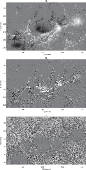
Figure 1. Top plot shows a typical spatial map of Bz for NOAA 11158. The middle is a spatial map of Hc, and the bottom is of α, both from the same region. Light/dark gray regions, respectively, correspond to positive/negative values of Bz, Hc, and α. The same layout is used in Figures 2 and 3.
Download figure:
Standard image High-resolution image
Figure 2. In order from top to bottom are shown spatial maps of Bz, Hc, and α for NOAA 11158, with noise reduction applied. Noise thresholds of  and
and  were used. Noise reduction changed α more noticeably than Bz or Hc.
Download figure:
Standard image High-resolution image
Figure 3. In order from top to bottom are shown spatial maps of Bz, Hc, and α for NOAA 11158, with Gaussian smoothing. A Gaussian function with 2'' FWHM was used.
Download figure:
Standard image High-resolution image3. RESULTS
3.1. Effects of Spatial Smoothing on Two Active Regions
3.1.1. NOAA 11158
The results of our initial analysis on NOAA 11158, without any spatial smoothing, are shown in Figure 4. Past authors have found different helicity patterns for fields with strong and weak Bz (e.g., Zhang 2006, Gosain et al. 2013, Seligman et al. 2014). To investigate this phenomenon further, we plot in Figures 4–7 Hc and α against Bz and Bt to investigate the dependence of the helicity parameters on field strength. Our unsmoothed results from NOAA 11158 (Figure 4) are consistent with previous results on the region: Hc was positive, and while α showed a mixture of negative and positive polarity around weak Bz values, it had a stronger positive bias. The results with both noise reduction and Gaussian smoothing applied are shown in Figure 5. Noise reduction had significant effects on α but not on Hc. The magnetic twist parameter α became positive at large  , while retaining its negative polarity in weak
  bins. It also became positive for a larger range of Bt, and α's maximum appeared to change from a Bt of 150 to 2000 G. This change was not as dramatic as it appeared; the unsmoothed data's large positive grouping at 150 G was actually skewed by a couple of disproportionately large Jz/Bz values, which were the result of small Bz values that got removed by noise reduction. The apparently new maximum α at 2000 G was actually a value of α that remained unchanged before and after noise reduction; instead, what changed was that value's relation to the other noise-reduced α values. The α calculation was strongly affected by small Bz values due to α's inverse relationship with Bz; thus, removing small Bz values via noise reduction spread out the clean α bias seen in Figure 4 and appeared to change the maximum average of α. Nonetheless, the noise-reduced helicities were still mostly positive.

Figure 4. Results for unsmoothed data from NOAA 11158. The top two histograms show Hc and α plotted against vertical field Bz, and the bottom two histograms show α and Hc plotted against transverse field Bt. All four graphs used a binsize of 50 G. Each bin contains an average of the collection of helicity values corresponding to that range of Bz or Bt. The same layout is used for Figures 5–7.
Download figure:
Standard image High-resolution image
Figure 5. Results for data from NOAA 11158 with both noise reduction and Gaussian smoothing applied. The same layout is used as in Figure 4.
Download figure:
Standard image High-resolution imageGaussian smoothing amplified and consolidated biases already existing in the data by smoothing each pixel's neighborhood via Gaussian-weighted averages. These weighted averages further emphasized the more common pixel values and removed outliers. When applied to the unsmoothed data, Gaussian smoothing slightly increased the positive bias for Hc and decreased α's negative trends for mid-range Bt. Combined with noise reduction, Gaussian smoothing confined the negative trend existing for α to a couple of large pixels around 0 G Bz, and smoothed out the positive bias for α around high values of Bt.
Gaussian smoothing and noise reduction had stronger effects on α than on Hc due to α's inverse relationship with Bz. Nonetheless, the helicities were generally positive throughout the smoothing process, although α remained negative for weak Bz values when both Gaussian smoothing and noise reduction were applied. Overall, the average Hc and α values of NOAA 11158 remained positive at each stage of the data processing. The average Hc for weak ( ) fields was small and negative before and after smoothing, and the weak-Bz α became negative as a result of the smoothing. The strong-Bz (
 ) parameter averages were positive throughout. It follows that, even though the smoothing operations had significant effects on the helicity distributions, the overall helicities for this southern-hemisphere region were consistent with the hemispheric rule both before and after smoothing. Our next region had more complex helicity biases.
3.1.2. NOAA 11243
Without any smoothing, helicity parameter histograms for this region displayed mixed trends, as shown in Figure 6. Hc had a strong positive bias for high Bz values, mixed biases for negative Bz values, and a strong negative bias around a Bt of 1600 G. On the other hand, α once again displayed a mixture of positive and negative polarity for weak Bz, but had a strong negative bias around low  values and a strong positive bias around high Bt values.
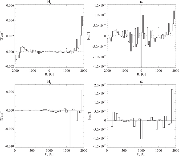
Figure 6. Results for unsmoothed data from NOAA 11243. The top two histograms show Hc and α plotted against vertical field Bz, and the bottom two histograms show α and Hc plotted against transverse field Bt. All four graphs used a binsize of 50 G. Each bin contains an average of the collection of helicity values corresponding to that range of Bz or Bt.
Download figure:
Standard image High-resolution image
O15 examined this region in detail and concluded that the helicities followed the hemisphere rule for weak magnetic field values ( ). Our results for the unsmoothed case do not conform to their findings but become consistent with them when smoothing is applied, possibly because O15 performed some of their processing, such as the azimuth angle disambiguation, at 2'' resolution, whereas our data were processed at full resolution. Our results with both noise reduction and Gaussian smoothing applied are shown in Figure 7. Noise reduction had the same effect as on NOAA 11158: α became more randomly distributed for weak-Bz fields and more widely distributed for large Bz. Similarly, Gaussian smoothing enhanced the trends already apparent in the unsmoothed data: negative Hc spread out at low Bz values, as well as at Bt values around 1000 G, while α remained negative for weak Bz. Hc appeared to gain negative values around a Bz of 1500 G. In fact, Hc already had over 2000 negative Bz Jz values in this range, but they were too small to appear significant in the histogram for the unsmoothed results of Hc versus Bz (see Figure 6). Gaussian smoothing consolidated and enhanced this collection of α values by weighting them more heavily, resulting in the seemingly new negative trend in the smoothed histogram in Figure 7. Another apparently new trend was the change from positive α at high Bt values to negative α at weak Bt values. In this case, the unsmoothed histogram's maximum α at a Bt of 1900 G only corresponded to 3 Jz/Bz values, whereas the negative α at 100 G corresponded to about 16,000 Jz/Bz values. When Gaussian smoothing was applied, the small collection of positive α at 1900 G was reduced, and the large collection of negative α at 100 G got weighted more heavily, resulting in a negative average helicity and a clear negative helicity bias in Figure 7 that was less apparent in Figure 6. Both of these changes demonstrate that using Gaussian smoothing on the data can lead to a clearer representation of the dominant trends in the histograms by removing the influence of outliers.

Figure 7. Results for data from NOAA 11243 with both noise reduction and Gaussian smoothing applied. The layout is the same as in Figure 6.
Download figure:
Standard image High-resolution imageWhile both α and Hc were negative at large negative values of Bz and weak values of Bt, and positive for large positive values of Bz and Bt, the helicities' negative biases were predominantly larger than their positive ones. On the other hand, the average Hc and α values indicate the complexity of the helicity distributions of this region. The average weak-Bz ( ) Hc of the region changed from negative to positive as a result of the smoothing and the average weak-Bz α was negative before and after the smoothing. The average strong-Bz (
 ) Hc and α values were barely positive on average throughout the processing. Since NOAA 11243 lay in the northern hemisphere, and the hemispheric helicity rule would lead us to expect dominant negative helicity. It is difficult to conclude whether or not NOAA 11243 adhered to the hemispheric rule because its distribution is so much more complex than those of NOAA 11158. To draw firmer conclusions, we need to study a larger sample of ARs. This is the subject of the next section.
3.2. Effects of Spatial Smoothing on Average Helicities of 179 Active Regions
In order to study the effects of spatial smoothing on overall helicities of ARs distributed across various latitudes, we calculated the average helicities of 179 ARs, 106 in the northern hemisphere and 73 in the southern. We selected the ARs according to whether they were observed within 30° of central meridian with a field of view larger than 104 arcsec2, 103 arcsec2 of which were required to have a vertical field  . In cases with more than one magnetogram meeting these criteria, we selected the one observed closest to the central meridian. We calculated the average helicities for strong and weak Bz separately. We identified strong Bz as
  and weak Bz as
  , following the example of Zhang (2006) and Gosain et al. (2013). The unsmoothed results for the 179 ARs are shown in Figure 8. The distribution by field strength, sign, and hemisphere of the unsmoothed and smoothed average helicity results are shown in Table 1. There are clear differences between the weak- and strong-Bz statistics. A total of 122 of the unsmoothed weak-Bz field Hc averages and 133 of the unsmoothed weak-Bz field α averages were negative. In the unsmoothed strong-Bz averages, 129 of the Hc and 133 of the α values were positive. For weak-Bz fields, both Hc and α had sizable negative biases in both hemispheres, and the strong-Bz fields had marked positive biases in both hemispheres, especially in the south.

Figure 8. Scatter plots of the helicity parameters against latitude for the unsmoothed data from 179 ARs, 106 in the northern hemisphere and 73 in the southern. Each point on a plot represents the total average helicity for one region. The top left and right plots show average α and Hc values, respectively, for weak Bz. The bottom left and right show the same but for strong Bz. Strong Bz is defined as  , and weak Bz as
  . The same layout is used for Figure 9.
Download figure:
Standard image High-resolution imageTable 1. Separation of Average Helicity Values by Field Strength, Sign, and Hemisphere
| Without Smoothing | With Smoothing | |||||
|---|---|---|---|---|---|---|
| Field Strength | Sign | Hemisphere | Hc | α | Hc | α |
| weak | >0 | N | 37 | 33 | 39 | 38 |
| weak | <0 | N | 69 | 73 | 67 | 68 |
| weak | >0 | S | 20 | 13 | 32 | 28 |
| weak | <0 | S | 53 | 60 | 41 | 45 |
| strong | >0 | N | 65 | 69 | 57 | 65 |
| strong | <0 | N | 41 | 37 | 49 | 41 |
| strong | >0 | S | 64 | 64 | 55 | 55 |
| strong | <0 | S | 9 | 9 | 18 | 18 |
Note. The above table shows the distribution of the average helicity values of the 179 ARs shown in Figures 8 and 9.
Download table as: ASCIITypeset image
Gaussian smoothing had little qualitative effect on the weak-Bz and strong-Bz field helicity biases. The results for the 179 ARs with both noise reduction and Gaussian smoothing applied are shown in Figure 9. The statistics for these smoothed data are qualitatively similar to the unsmoothed results: negative biases for weak-Bz fields in both hemispheres, and positive biases for strong-Bz fields in both hemispheres, especially in the south. Comparing the statistics for the smoothed data to those for the unsmoothed data, the smoothing generally diminished the hemispheric biases. This could be interpreted as evidence that the smoothing tends to reduce biases in the data by eliminating outliers. However, according to statistical Z-tests, these changes do not seem to be statistically significant in general. Only the weak-Bz α statistics for the southern hemisphere changed significantly after smoothing. Otherwise, the patterns are essentially the same in the smoothed data as in the unsmoothed data. Noise reduction had negligible effects on the distributions of the average helicities. This might be because the helicity values were not separated into bins for different Bz and Bt values before taking their average, as they were in Section 3, but instead were averaged as one set. The changes caused by the removal of minute Bz values would be less apparent when the helicities were averaged as a group because disproportionately large Jz/Bz values would not skew the average as significantly as when they were placed in smaller bins of helicity values.

Figure 9. Scatter plots of the helicity parameters against latitude for the data from the 179 ARs with both Gaussian smoothing and noise reduction applied. The same layout is used as in Figure 8.
Download figure:
Standard image High-resolution image
It is clear from Figures 8 and 9 that the data set as a whole does not conform to the hemispheric helicity rule, and the smoothing does not change this fact.
4. DISCUSSION
The results are summarized as follows: NOAA 11158 followed the hemisphere rule both before and after spatial smoothing, whereas NOAA 11243s status is more ambiguous and its helicity helicity parameter distributions more complex. The average helicity parameter values of the 179 ARs did not follow the hemisphere rule: the weak-Bz helicity values tended to be negative in both hemispheres, and the strong-Bz values positive especially in the south. Our results thus reflect the complex mixture of results for helicity parameter statistics published recently by Zhang (2006), Gosain et al. (2013), Seligman et al. (2014), and O15. Our results are robust against Gaussian smoothing and noise reduction, thus supporting consistency between previous ground-based results (e.g., Zhang 2006) and space-based results on helicity. It is important to note that Gaussian smoothing is not an exact replica of the effects of seeing from atmospheric turbulence, but is a simple way to simulate its spatial smoothing effects.
For NOAA 11158, applying noise reduction and Gaussian smoothing resulted in strengthened representations of the overall trends in the data. For both NOAA 11158 and NOAA 11243 noise reduction and Gaussian smoothing seemed to significantly change the helicity distributions of both regions, especially for α. Both noise reduction and Gaussian smoothing shifted the distributions by reducing influences produced by relatively large, non-representative helicity values and favoring biases that corresponded to larger proportions of the helicity distributions.
Noise reduction removed Bz values that were insignificant because they were below the noise thresholds of the measurements and the sensitivity of the inversions; these values seriously skewed the results, especially for the Jz/Bz calculation, until they were removed. Gaussian smoothing reduced outliers that were likewise skewing the helicity distributions. Arguably, these outliers correspond to smaller distances because they are proportional to 1/L or B2/L, and are also less representative of the general helicity trends for an entire AR because they correspond to tight and localized current linkages or magnetic twist. Since the smoothed results were consistent with the unsmoothed results, it follows that the smoothing effects of seeing from atmospheric turbulence do not produce false patterns, but represent the helicity properties of the bulk of the field by suppressing the influence of outliers. This result suggests that ground-based measurements, with their seeing effects, capture the helicity properties of ARs. Thus while our results for the separation of weak-Bz and strong-Bz helicities do not closely agree with those of Zhang (2006), Gosain et al. (2013) or Seligman et al. (2014), these discrepancies are likely not due to smoothing or atmospheric seeing, but rather are due to the differing studied time intervals, which represent different phases of the solar cycle.
Considering that noise reduction and Gaussian smoothing were important for untangling the complexities in the helicity parameter distributions within individual ARs, it makes sense that noise reduction and Gaussian smoothing had less effect on the overall average helicities calculated for large ranges of the strong- and weak-Bz fields. Averaging over small ranges of Bz (and Bt) allows for studying the changing distributions of helicity within a region, whereas averaging over large ranges of Bz provides a general overview of that region's helicity. Helicity results are usually presented in the form of averages over ARs, sometimes splitting fields into strong and weak categories, and so the major effects of spatial smoothing on helicity distributions such as those shown in Figures 4–7 generally go unnoticed.
The distinct patterns of behavior of helicity signs for strong- and weak-Bz fields still needs to be explained; O15 suggest that this is related to the separation of influences from poloidal and toroidal components; though, this needs to be studied more fully. An interesting possible explanation was provided by Blackman & Brandenburg (2003), who concluded that dynamo models for the generation of large-scale magnetic structures with writhe is accompanied by small-scale twist along these structures. This implies large- and small-scale helicities of opposite sign, a pattern found in helicity spectra calculated from vector magnetograms by Zhang et al. (2016).
Hinode data used here are produced by support from ISAS/JAXA, NAOJ, NASA, STFC, ESA, and NSC. This work was carried out through the National Solar Observatory Research Experiences for Undergraduates (REU) Program, which is funded by the National Science Foundation (NSF). The National Solar Observatory is operated by the Association of Universities for Research in Astronomy, Inc. (AURA) under cooperative agreement with the NSF.