


ABSTRACT
We present new Atacama Large Millimeter/Submillimeter Array (ALMA) 850 μm continuum observations of the original Lyα Blob (LAB) in the SSA22 field at z = 3.1 (SSA22-LAB01). The ALMA map resolves the previously identified submillimeter source into three components with a total flux density of S850 = 1.68 ± 0.06 mJy, corresponding to a star-formation rate of ∼150 M⊙ yr−1. The submillimeter sources are associated with several faint (m ≈ 27 mag) rest-frame ultraviolet sources identified in Hubble Space Telescope Imaging Spectrograph (STIS) clear filter imaging (λ ≈ 5850 Å). One of these companions is spectroscopically confirmed with the Keck Multi-Object Spectrometer For Infra-Red Exploration to lie within 20 projected kpc and 250 km s−1 of one of the ALMA components. We postulate that some of these STIS sources represent a population of low-mass star-forming satellites surrounding the central submillimeter sources, potentially contributing to their growth and activity through accretion. Using a high-resolution cosmological zoom simulation of a 1013 M⊙ halo at z = 3, including stellar, dust, and Lyα radiative transfer, we can model the ALMA+STIS observations and demonstrate that Lyα photons escaping from the central submillimeter sources are expected to resonantly scatter in neutral hydrogen, the majority of which is predicted to be associated with halo substructure. We show how this process gives rise to extended Lyα emission with similar surface brightness and morphology to observed giant LABs.
Export citation and abstract BibTeX RIS
1. INTRODUCTION
SSA22-LAB01 (z = 3.1, Steidel et al. 2000) is the most thoroughly studied (Bower et al. 2004; Chapman et al. 2004; Geach et al. 2007, 2014; Matsuda et al. 2007; Weijmans et al. 2010; Hayes et al. 2011; Beck et al. 2016) giant (100 kpc in projected extent) Lyα "Blob" (LAB). LABs are intriguing objects: the origin of the extended Lyα emission could be due to gravitational cooling radiation, with pristine hydrogen at T ∼ 104–5 K cooling primarily via collisionally excited Lyα as it flows into young galaxies (Katz et al. 1996; Haiman et al. 2000; Fardal et al. 2001). Alternatively, galactic winds, photoionization, fluorescence, or scattering processes have been proposed (Taniguchi & Shioya 2000; Geach et al. 2009, 2014; Alexander et al. 2016; Hine et al. 2016). In any scenario, the picture is one of an extended circumgalactic medium (CGM) that is rich in cool gas (be it clumpy or smoothly distributed), and so LABs reveal astrophysics associated with the environment on scales comparable to the virial radius of the massive dark matter halos they trace. Nevertheless, the process (or processes) giving rise to the extended line emission remains in question.
Cen & Zheng (2013) predicted that giant LABs should contain far-infrared sources close to the gravitational center of the halo. The presence of a central submillimeter-bright galaxy within SSA22-LAB01 has been in debate (Chapman et al. 2004; Matsuda et al. 2007; Yang et al. 2012) but was recently confirmed with the solid detection of an unresolved S850 = 4.6 ± 1.1 mJy submillimeter source using the SCUBA-2 instrument on the 15 m James Clerk Maxwell Telescope (Geach et al. 2014). Here we present new high-resolution Band 7 continuum (λobs = 850 μm) observations of SSA22-LAB01 with the Atacama Large Millimeter/Submillimeter Array (ALMA). These observations resolve the rest-frame 210 μm emission at z = 3.1, close to the peak of the thermal dust emission and therefore a good probe of the cold and dense interstellar medium (ISM). Throughout, we assume a cosmology with ΩΛ = 0.72, Ωm = 0.28 and  km s−1 Mpc−1. At z = 3 1'' subtends approximately 8 projected kiloparsecs (pkpc).
2. OBSERVATIONS
2.1. Atacama Large Millimeter/Submillimeter Array
SSA22-LAB01 was observed in two projects (2013.1.00922.S [PI Geach] and 2013.1.00704S [PI Matsuda]) with a similar configuration in Band 7: the full 7.5 GHz of bandwidth centered at 347.59 GHz was used to measure the continuum emission at approximately the same frequency as the SCUBA-2 detection of the target. A total of 36–40 12 m antennas were used in the observations, with baselines spanning 21–918 m, which were capable of recovering emission on scales of up to 5'', with a maximum resolution of 0 4. Antenna Tsys temperatures were approximately 100–150 K and the mean precipitable water vapour column was 0.249 mm. Observations of the phase calibrator source J2206-0031 confirm consistent flux scaling between the two projects in the calibration phase. All calibrations were performed using the casa software and the visibilities from each project concatenated into a single measurement set for which the total integration time is 2860 s.
The dirty image reveals the two main components of submillimeter emission, and we use this information to supply circular masks (each 2'' in radius) at 22h17m26 0, +00°12'363 and 22h17m261, +00°12'324 (J2000) to the casa clean task. We use a natural weighting of the visibilities and clean down to a threshold of 70 μJy within 1000 iterations. We adopt multi-scale cleaning, allowing model Gaussian components of width 0'' (delta function), 05, 1'', 2'', and 3''. The clean is run twice: at full resolution and with an outer taper of 1''. To both maps, we "feather" the single dish SCUBA-2 (regridded) map to improve the recovery of the total flux of the source and potentially improve sensitivity to extended emission. The depth of the map is 40 μJy beam−1, increasing to 90 μJy beam−1 after tapering. Final maps are corrected for primary beam attenuation for analysis. The synthesized beams are 040 × 038 (PA 23°) and 101 × 098 (PA 112°) in the feathered full resolution and 1'' tapered maps, respectively.
To measure the integrated flux densities and sizes, we threshold the maps at 3σ, where σ is the root-mean-square noise measured around the sources and sum the flux enclosed by each 3σ contour. In the full resolution map, there are three distinct components: a, b, and c. Integrated flux density uncertainties are estimated from the root-mean-squared value, scaled to the number of beams subtended by the 3σ contour. The sizes of each source in the tapered map are measured as the maximum width of the 3σ contour, with an uncertainty  , where θbeam is the full width half maximum of the beam and the S/N = 3.
Note that there is a discrepancy between the single dish flux and the total flux measured in the ALMA map:  mJy. Although this is not significant at the 3σ level, we should discuss this potential "missing" flux. First, it is important to note that single dish flux densities in the submillimeter can be statistically boosted; Geach et al. (2016) measured the flux boosting as a function of the S/N in the SCUBA-2 Cosmology Legacy Survey (where the SCUBA-2 detection of this target originates), finding an average boosting of approximately 30% for SSA22-LAB01. The array configuration allows us to recover emission on scales of up to 5''. It is unlikely that there is an 850 μm emission component on scales larger than this (40 pkpc at this redshift), but given the sensitivity of our observations, it implies that, if real, the missing submillimeter emission is extended on scales of at least 3'' (25 pkpc). One possibility is that the emission is spread over a large number of faint clumps around the central sources—an idea we explore later in the paper. Deeper observations with a slightly more compact array configuration would be beneficial to address this.
2.2. Multi-unit Spectroscopic Explorer (MUSE)
Integral field spectroscopy was performed with the Very Large Telescope MUSE instrument. The observations were carried out under clear or photometric conditions, between 2014 November and 2015 September. We used the extended blue setting, resulting in a minimum wavelength of 4650 Å. Each integration was 1500 s, and the field was rotated by 90° between each exposure in order to reduce fixed pattern noise from the integral field units and residual flat-field errors. Data were reduced with the MUSE pipeline (version 1.0.5), following standard procedures for bias subtraction, dark current removal, flat-fielding, and basic calibration of the individual integrations. Each individual spectrum was fully post-processed to output an image of the field of view, data cubes, and pixel tables, which we examined individually. We computed shifts between the individual exposures using standard centering tools in iraf. Finally, we used the muse_exp_combine task to drizzle and stack all the individually reduced pixtables.
2.3. Hubble Space Telescope (HST) Imaging Spectrograph
The HST Imaging Spectrograph (STIS) observations (project 9174, Chapman et al. 2004) used the 50CCD clear filter, which provides a wide response in the optical, with an effective central wavelength of 5850 Å and a full width half maximum throughput of 4410 Å over a 52'' × 52'' field of view. Six exposures of SSA22-LAB01 were taken in "LOW-SKY" time for a total of 7020 s of integration. HST Legacy Archive calibrated images were combined into a single deep co-add with 01 pixels using the DrizzlePac software (version 2) from the Space Telescope Science Institute. The 5σ sensitivity limit is 27.6 mag (Chapman et al. 2004).
2.4. Keck Multi-object Spectrometer for Infrared Exploration (MOSFIRE)
K-band (1.92–2.30 μm) spectroscopy of SSA22-LAB01 was obtained on a single slit of a multislit mask observed during science verification of the MOSFIRE (McLean et al. 2012) on the W. M. Keck Observatory Keck I 10 m telescope. The slit width was 07, resulting in a spectral resolving power of R ∼ 3600. The total integration time was 5040 s, in a sequence of 28 180 s exposures using an ABAB nod pattern with a nod amplitude of 30. The seeing during the observation was estimated to be 035 full width half maximum. The data were reduced by the MOSFIRE Data Reduction Pipeline (Steidel et al. 2014).
3. ANALYSIS AND INTERPRETATION
In the following sections, we analyze and interpret the observations, characterizing the ALMA sources in the context of the LAB environment. We then use a high-resolution cosmological hydrodynamic simulation and radiative transfer to develop a hypothesis about the role of the central submillimeter sources in the contribution to the extended Lyα emission. We pay particular attention to the creation of mock observations that can be directly compared to the data and to determining whether systems resembling SSA22-LAB01 are expected in current models of galaxy formation.
3.1. Observations
At full (04) resolution, we resolve three main components that we label "a," "b," and "c" within the SSA22-LAB01 (Figure 1). Component "a" is the brightest submillimeter source, located close to the geometric center of the LAB and is 1'' from component "b"; in the tapered map these effectively blend into a single source, and we consider a+b jointly hereafter. Component "c" is located 45 to the southeast and is associated with strong stellar continuum emission, with a precise redshift measured from [O iii] and Hβ lines, z = 3.1000 ± 0.0003, placing it within the Lyα nebula (Kubo et al. 2015). Component a+b is also coincident with stellar continuum emission of complex, clumpy morphology—it is not clear whether this is a single bound system and we are simply detecting bright clumps of submillimeter and optical emission, or if we are witnessing the coalescence of several independent low-mass systems.

Figure 1. Observations of SSA22-LAB01. (Left) MUSE continuum-subtracted line image showing the Lyα emission averaged over 4976–5000 Å, with contours at levels of 0.5, 0.7, and 1 × 10⁻¹⁹ erg s−1 cm−2 Å−1. Black lines show Lyα polarization (Hayes et al. 2011) and black contours show the 1'' tapered ALMA 850 μm emission at >3σ significance. (Center) Zoom-in of the ALMA map with the highest-resolution image as the background and with the full resolution and tapered 850 μm contours overlaid (starting at 3σ, increasing in steps of 1σ); yellow ellipses show the FWHM of the full resolution and tapered synthesized beams. (Right) HST/STIS optical image of the same region as the central panel, indicating the orientation of the Keck MOSFIRE slit (Section 2.4) and the position of a faint companion source we label "S1." We overplot the same contours as the central panel to illustrate how the submillimeter sources are associated with emission in the STIS map.
Download figure:
Standard image High-resolution imageThe total flux density of the signal above the 3σ level in the tapered map is S850 = 1.68 ± 0.06 mJy; Table 1 gives the positions and flux density of the two main components a+b and c. Assuming that cool dust emission traces the dense ISM (Scoville et al. 2015), the corresponding total molecular gas mass is  M⊙ and the average molecular gas surface density is Σgas ≈ 140
  pc−2. If ΣSFR scales linearly with Σgas (Wong & Blitz 2002), we estimate that the submillimeter sources are forming stars at rates of the order of 100
  yr−1. We have poor constraints on the shape of the spectral energy distribution (SED) of these sources, but we can estimate their integrated total infrared luminosities by assuming an appropriate range of templates describing the thermal dust emission of active galaxies. We adopt the Dale & Helou (2002) set of templates, characterized by a parameter α, describing the power-law index for the distribution of dust mass over heating by the interstellar radation field (U):
  , with most galaxies falling within the range of α = 1–2.5; we conservatively consider this full range when estimating the total infrared luminosities of the sources. Redshifting to z = 3.1 and normalizing to the observed 850 μm flux density, we estimate total infrared (8–1000 μm) luminosities in the range of
  and
and  for sources a+b and c respectively. The median infrared luminosity considering the full range of templates is
  and
and  for the two components, respectively, where the error bar reflects the measurement uncertainty on the integrated ALMA flux. Assuming a star-formation rate calibration following Kennicutt & Evans (2012) these average luminosities correspond to SFR ≈ 90 M⊙ yr−1 and
  yr−1, respectively, consistent with the ISM mass scaling value derived above, though the SFRs could be a factor of three higher if the galaxies are better represented by the more "active" templates of the Dale & Helou library.
Table 1. Properties of ALMA Sources in SSA22-LAB01
| Source | R.A. | Decl. | S850 |
|---|---|---|---|
| (h m s) | (°' '') | (mJy) | |
| SSA22-LAB01 ALMA a+b | 22 17 26.01 | +00 12 36.5 | 0.95 ± 0.04 |
| SSA22-LAB01 ALMA c | 22 17 26.11 | +00 12 32.2 | 0.73 ± 0.05 |
Download table as: ASCIITypeset image
The emergent luminosity of Lyα emission associated with obscured star formation is  (Dijkstra & Westra 2010), under the assumption of Case B conditions and where
  is the escape fraction (of Lyα photons) from the galaxy. This corresponds to
  erg s−1 per ALMA source, similar to the total Lyα luminosity of SSA22-LAB01. From the models of Leitherer et al. (1999), the ionizing flux (ν = 200–912 Å) scales like
  erg s−1 (for 100 Myr of continuous star formation, solar metallicity and Salpeter IMF). Thus, for star-formation rates of the order of 100 M⊙ yr−1 and modest high escape fractions, the ALMA sources appear to be viable "power sources" for extended Lyα emission through photoionization. The next question follows naturally: what is the nature of the environment around these central star-forming sources?
Like other giant LABs (e.g., Prescott et al. 2012), SSA22-LAB01 is thought to trace a massive dark matter halo of the order of  this is close to the mass where cold flows are not expected to survive inside the virial radius at this epoch (Dekel et al. 2009). Recently, moving mesh hydrodynamic simulations suggest cold streams are assimilated into the hot halo gas inside the virial radius even down to halo masses of
  (Nelson et al. 2013), suggesting that cold flows are not sufficient to explain the extended Lyα luminosity of giant LABs. Following arguments put forward by Hayes et al. (2011), Geach et al. (2014), and Beck et al. (2016), we postulate that extended line emission in SSA22-LAB01 could arise from Lyα photons generated by central star formation in the submillimeter sources, escaping and resonantly scattering in neutral gas associated with a large ensemble of lower-mass galaxies in the same potential well (e.g., Cen & Zheng 2013, Francis et al. 2013). This is consistent with recent spectropolarimetry observations of SSA22-LAB01 that favor a scenario in which Lyα photons undergo long flights from central sources before scattering in H i in the CGM (Hayes et al. 2011; Beck et al. 2016, though see Trebitsch et al. 2016). In Figure 1, we show the polarization vectors of Hayes et al. (2011) that describe a circular pattern roughly centered on the submillimeter sources.
The STIS imaging reveals many faint (fλ ≈ 10−19 erg s−1 cm−2 Å−1) clumps of UV emission surrounding the submillimeter sources (Figure 1, Chapman et al. 2004; Matsuda et al. 2007, Uchimoto et al. 2008, see also Prescott et al. 2012). There is no spectroscopically confirmed redshift for source a+b, and, unlike source c, it is not unambiguously associated with an STIS counterpart. Instead, there are a number of STIS clumps at (and around) the position of a+b, and the optical colors of these are broadly consistent with a z = 3.1 redshift (Kubo et al. 2015). In addition, there is a possible H i absorption feature in the Lyα spectrum at this location (Weijmans et al. 2010; Geach et al. 2014); thus, source a+b is unlikely to be a chance projection of a submillimeter source at a different redshift. In the event that this ALMA source is not associated with the LAB, then obviously the main impact on our analysis and interpretation is that there will be approximately a factor of two fewer Lyα and UV photons generated by central star formation.
If some (a fraction are likely to be chance projections) of the other faint STIS sources represent low-mass satellites of the ALMA sources, then the cold gas associated with them could be responsible for scattering Lyα photons emerging from the central active galaxies. A key test is actually confirming the "membership" of the STIS sources, and to this end we have obtained near-infrared spectroscopic confirmation of one of these faint companion sources "S1" (Figure 2), detecting the [O iii] line at z = 3.0968. S1 is 21 (17 pkpc) from ALMA source "c" with a line-of-sight velocity offset of just 250 km s−1. Although not a complete survey by any means, this observation does support the view that the central ALMA sources are accompanied by a population of low-mass satellites. With this empirical evidence in hand, we now consider whether the same observations are predicted by galaxy formation and evolution models. In particular, we run a zoomed cosmological hydrodynamical simulation coupled with radiative transfer schemes to produce mock observations that can be directly compared to the data. The main objective is to test whether systems similar to SSA22-LAB01 arise in current galaxy formation schemes.
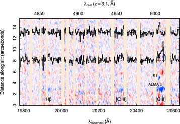
Figure 2. Near-infrared spectrum of ALMA source c and companion obtained with Keck MOSFIRE. The background image shows the two-dimensional spectrum, slightly smoothed for clarity. Strong atmospheric emission lines are masked. The nod pattern employed results in a positive (red) and negative (blue) signal in the co-added spectrum offset by 3''. The 1D spectra for each source reveal Hβ and [O iii] emission lines, with the 5007 Å [O iii] line separated by 250 km s−1 between ALMA source "c" and S1, which are separated by an angular distance of 21 (17 pkpc).
Download figure:
Standard image High-resolution image3.2. Simulations
We simulate the formation of a galaxy in a massive ( ) halo (by z = 2) utilizing a cosmological zoom technique with the hydrodynamics code gizmo (Hopkins 2014). We employ a pressure-entropy formulation of smoothed particle hydrodynamics, which conserves momentum, energy, angular momentum, and entropy. We first run a coarse large (144 Mpc3) dark matter-only simulation to identify a halo of interest. This simulation is run at a relatively low-mass resolution
  . At z = 2, we select a massive (
 ) halo, and re-simulate the evolution of this halo at significantly higher resolution (Feldmann et al. 2016), including baryons with a particle mass of mbar = 2.7 × 10⁵ M⊙. The initial conditions are generated with the music code (Hahn & Abel 2011) and the minimum baryonic, star, and dark matter force softening lengths are, respectively, 9, 21, and 142 proper parsecs at z = 2. The halo simulated here is the exact same as the main halo in Narayanan et al. (2016).
Gas cools using a cooling curve that includes both atomic and molecular line emission, with the neutral ISM broken into atomic and molecular components following an analytic algorithm describing the molecular fraction in a cloud based on the gas surface density and metallicity (Krumholz et al. 2009). Star formation occurs in molecular gas and follows a volumetric relation  , where ρmol is the volume density of molecular gas and tff is the freefall time. Star formation is restricted to gas that is locally self-gravitating following the algorithms of Hopkins et al. (2013). Once stars have formed, they impact the ISM via a number of feedback channels. In particular, we include models for momentum deposition by stellar radiation and supernovae, photoheating of H ii regions, and stellar winds (see Hopkins 2014 for details). gizmo tracks 11 metal species (H, He, C, N, O, Ne, Mg, Si, S, Ca, and Fe) with yields from SN 1a and SN II following Iwamoto et al. (1999) and Woosley & Weaver (1995).
To model the ALMA and STIS observations we employ the dust radiative transfer code Powderday which computes the stellar SEDs of the star particles (constrained by their ages and metallicities) and propagates this radiation through the dusty ISM. The gas particles are projected onto an adaptive grid with an octree-like memory structure (using yt, Turk et al. 2011), and the dust mass is assumed to be a constant fraction (40%) of the total metal mass in a given cell (Dwek 1998; Watson 2011). Photons are emitted in a Monte Carlo fashion and absorbed, re-radiated, and scattered by dust; this process is iterated upon until the dust temperature has converged. The stellar SEDs are calculated at the run time for each stellar particle utilizing fsps (Conroy & Gunn 2010). We employ the Padova iscochrones and assume a Kroupa IMF. The dust radiative transfer employs hyperion (Robitaille 2011). We assume a Weingartner & Draine (2001) dust size distribution, with RV = 3.15. To create mock observations, we consider the observed frame 850 μm and optical emission predicted by Powderday and hyperion projected onto a celestial grid at the position of SSA22-LAB01.
To simulate the ALMA observations, we use the casa task simalma, setting the simulation parameters to match the real observations (Section 2.1), including the same array configuration. The resulting maps have a nearly identical synthesized beam and 1σ noise as the data. For the STIS imaging, we convolve the predicted observed frame UV-through-optical emission with the 50CCD throughput curve to generate single images projected along the same view angles as the 850 μm images. These images are then convolved with the STIS point-spread function (PSF) and gridded to an identical pixel scale as the observations. Finally, we create a noise image by removing >1.5σ features from the real STIS image and replace those pixels with values randomly drawn from the remainder of the pixels in the image. The noise-free, PSF-convolved flux image is then added to the noise image to create the mock observation.
Finally, we consider Lyα radiative transfer of centrally generated photons through the simulation volume. We use the code tlac (Gronke et al. 2014, 2015) with the default core skipping parameter x = 3. The central 400 pkpc of simulation volume is interpolated onto a regular grid, and we treat two central, star-forming galaxies (SFRs 189 M⊙ yr−1 and 115 M⊙ yr−1) as sources of Lyα photons. To compute the Lyα luminosity emitted by the cells, we use the relation between star-formation rate and Lyα luminosity (applicable to solar metallicity and a Kroupa IMF)

The photons are emitted from a random point inside the corresponding cell with an emission frequency drawn from a distribution depending on the thermal velocity of the gas in the cell (Gronke et al. 2014, 2015) using the "peeling" algorithm (Yusef-Zadeh et al. 1984; Zheng & Miralda-Escudé 2002; Laursen 2010). We follow the prescriptions of Laursen (2010) for the Small Magellanic Cloud (Pei 1992; Weingartner & Draine 2001; Gnedin et al. 2008) when calculating the dust content in the grid, and a full description of this method can be found in that work. We compute an effective dust density nd at every cell as

where  and
and  are the neutral and ionized hydrogen densities, respectively, at every cell. Z and
  denote the metallicity at every cell and the SMC average, respectively, and fion accounts for the dust content in the ionized gas (Laursen 2010). We assume that fion is 1% and note that
  is 0.6 dex below the solar value.
3.3. Comparing Data and Simulations
Figure 3 shows the synthetic ALMA and STIS observations. We do not expect perfect fidelity with the observations, but we can note some important similarities. As in the observation, the simulated halo contains two main star-forming galaxies with SFRs 189 and 115 M⊙ yr−1, respectively; these are well within the range of SFRs we estimate in Section 3.1. Both galaxies are submillimeter emitters, but only one has a flux density high enough to be detected in our mock ALMA map, with S850 ≈ 0.5 mJy, within a factor of two of the observations. In the simulation, both galaxies are bright STIS sources, whereas this is only true of one of three observed ALMA components. The two central galaxies are surrounded by several STIS-detectable clumps (within ∼5'' or about 40 pkpc) that are of similar flux to those observed. Formally, we detect five sources at the >3σ level in the synthetic STIS image27 , with flux densities of fλ ≈ (0.2–4) × 10−19 erg s−1 cm−2 Å−1. This is compared to eight sources with fλ ≈ (0.2–2) × 10−19 erg s−1 cm−2 Å−1 over the same area in the real image using identical detection criteria (Figure 1). In the real data, some of these sources could be chance projections, and we quantify this contamination by running the detection on the wider STIS image to measure the average surface density of sources in the same flux range. In a random 5'' radius aperture, we would expect 4 ± 1 sources by chance, so the predicted abundance of STIS sources in the simulation is in good agreement with the observations.

Figure 3. Predicted ultraviolet and submillimeter emission of a  halo at z ≈ 3 from a hydrodynamic simulation with realistic radiative transfer (Section 3.2). (Left) Predicted emission in the HST STIS 50CCD band with zero noise. Black contours show the predicted 850 μm emission, logarithmically spaced at 0.25 dex, starting at 0.1 μJy. Both the STIS and submillimeter image has been slightly smoothed for clarity; (right) shows the same emission, but as would be observed with an identical set-up to the real observations. Background scaling of the mock HST STIS image and 1'' tapered ALMA contours are identical to Figure 1 (we only show the tapered contours for clarity here). Only the brightest handful of neighboring STIS sources are detectable, with flux densities of fλ ≳ 2 × 10⁻²⁰ erg s−1 cm−2 Å−1. Formally, we detect five STIS sources above a 3σ detection threshold, which is similar to the observations after considering contamination from projections (Section 3.3).
Download figure:
Standard image High-resolution imageWhat are these faint neighboring sources? In the simulation, these STIS clumps are the brightest of a population of star-forming sub-halos (that are apparent in the left panel of Figure 3) that "swarm" the central star-forming galaxy, bombarding it over a ∼1 Gyr period in a phase of hierarchical growth that accompanies the accretion of recycled gas previously heated by stellar feedback at an earlier epoch (Narayanan et al. 2015). So the simulation can broadly reproduce the ALMA and STIS observations, and we can interpret this as a demonstration that, as far as can be determined by the data, the halo population observed in SSA22-LAB01 is consistent with the prediction of this particular model of galaxy evolution for a halo of equivalent mass. What of the extended Lyα emission?
Considering the two main star-forming galaxies sources as Lyα emitters (with Lyα luminosities scaled from their SFRs, Equation (1)), we find that 58% of centrally generated photons escape the simulation box, and 16% of those scatter at least once in H i in the CGM. The majority (77%) of the H i mass in the central 400 pkpc of the simulation volume is tied to sub-halos, and thus it follows that the majority of the Lyα scattering occurs in and around satellites, which can be treated as cold clumps within the hot halo gas. Figure 4 shows the projected Lyα surface brightness maps of the simulated halo compared to the latest integral field observations from MUSE. Resonant scattering in the satellite population gives rise to extended Lyα emission with surface brightness distributions similar to observed LABs ( erg s−1 cm−2 arcsec−2). The observed Lyα surface brightness and morphology is highly orientation dependent Lyα sources—the emission need not be symmetric about the central sources that are the source of the Lyα photons. This is simiular to the situation in real LABs, for example, the next largest LAB in SSA22, SSA22-LAB02 contains an X-ray luminous AGN (Geach et al. 2009; Alexander et al. 2016) that is significantly offset from the peak and geometric center of the LAB. This has important implications for correctly identifying potential luminous galaxy counterparts to LABs, the apparent absence of which in some systems has previously been argued in favor of cold mode acceretion (e.g., Nilsson et al. 2006, but see also Prescott et al. 2015).
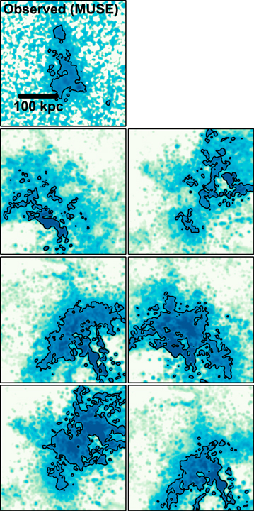
Figure 4. Predicted surface brightness profiles of extended Lyα emission compared to observations. The first panel shows the MUSE observation of SSA22-LAB01 with an isophotal contour at  erg s−1 cm−2 arcsec−2 used to originally classify LABs (Matsuda et al. 2004). Additional panels show, at the same scale, the Lyα surface brightness maps predicted by our simulation (no noise has been added), smoothed with a Gaussian beam of fwhm 1'' to mimic ground-based seeing. These maps are generated by projecting the simulation volume along each of the six faces of the cube. The central star-forming galaxies (analogous to the ALMA sources) are at the center of the cube, and so it is clear that large-scale scattering in the halo substructure can form LABs that are highly asymmetric about the "power" sources, and produce emission line halos with a range of morphology. Note also the fainter extended emission predicted by the model on scales larger than the single isophote shown.
Download figure:
Standard image High-resolution image
4. SUMMARY
It is uncontroversial that the intergalactic medium is rich in cool baryons at z ≈ 3, and recent observations have demonstrated how gas in the cosmic web can be detected in Lyα emission on scales much larger than 100 pkpc via illumination by nearby quasars (Cantalupo et al. 2014; Martin et al. 2015). Deep stacking experiments have also demonstrated that diffuse, extended Lyα emission appears to be a generic feature within 100 pkpc of star-forming galaxies at high redshift, potentially linked to scattering in a clumpy CGM (Steidel et al. 2011). However, it has not been clear how cold gas is actually distributed within dark matter halos and how it relates to the growth of central galaxies.
Our new ALMA observations have resolved two active galaxies at the heart of SSA22-LAB01, with a total star-formation rate of the order of 150 M⊙ yr−1, and there is evidence to suggest that these are surrounded by a retinue of lower-mass satellites, the brightest of which are detectable in deep HST STIS imaging. Our self-consistent hydrodynamic simulation and mock observations lead us to postulate that cold gas associated with the halo substructure—much of which is predicted to be associated with the satellites—acts as a scattering medium for Lyα photons escaping from the central star-forming galaxies, and demonstrate that this can give rise to large Lyα nebulae similar to observed LABs. Although resonant scattering is unlikely to be the only contributor to the extended Lyα emission, we argue that it may be a dominant process. We suggest that deep, high-resolution Lyα observations offer a route to mapping the distribution and kinematics of the satellite populations—or, more generally, substructure—of distant massive halos.
We thank the referee for a constructive report that has improved this work. J.E.G. is supported by a Royal Society University Research Fellowship. Partial support for D.N. was provided by NSF AST-1442650, NASA HST AR-13906.001, and a Cottrell College Science Award. M.H. acknowledges the support of the Swedish Research Council, Vetenskapsrådet and the Swedish National Space Board (SNSB), and is a Fellow of the Knut and Alice Wallenberg Foundation. H.D. acknowledges financial support from the Spanish Ministry of Economy and Competitiveness (MINECO) under the 2014 Ramón y Cajal program MINECO RYC-2014-15686. A.V. is supported by a Research Fellowship from the Leverhulme Trust. The authors acknowledge excellent support of the UK ALMA Regional Centre Node. This letter makes use of the following ALMA data: ADS/JAO.ALMA#2013.1.00704S, ADS/JAO.ALMA#2013.1.00922.S. ALMA is a partnership of ESO (representing its member states), NSF (USA), and NINS (Japan), together with NRC (Canada) and NSC and ASIAA (Taiwan), in cooperation with the Republic of Chile. The Joint ALMA Observatory is operated by ESO, AUI/NRAO, and NAOJ. This work was supported by the ALMA Japan Research Grant of NAOJ Chile Observatory, NAOJ-ALMA-0086.
Footnotes
- 27
We detect sources using SExtractor version 2.19.5 (Bertin & Arnouts 1996) with a detection threshold of three continguous pixels above three times the rms in the local background. No filtering is applied, and we use a back size of 32 pixels.