


ABSTRACT
New observations of the magnetic field  from ≈2014.7 through 2016.3288, together with the previous observations dating back to 2012 August 25, show that Voyager 1 continued to observe draped interstellar magnetic fields in the outer heliosheath. During this time, the direction of
  was nearly constant (±3°), with no significant long-term trend. The slope of a linear least squares fit to the variation of the magnetic field strength B with time is (0.001 ± 0.001) nT yr−1, consistent with no net change, and the average B = (0.48 ± 0.04) nT. The new observations show a second "disturbed interval" in which B was
  for ≈267 days. This interval began with a weak shock on 2014/236 (2014.6438), contained oscillations in B with a 28 day period, and possibly ended with a pressure balanced structure or a reverse shock. It is likely this disturbed interval was associated with Sun/solar wind disturbances that impacted the heliopause and produced disturbances that propagated into the outer heliosheath. A quiet interval containing weaker less variable
  was observed from ≈2015.3700 until at least 2016.0. Unlike the previous quiet interval observed in the outer heliosheath, the direction of
  did not change linearly and could not be extrapolated to the center of the IBEX ribbon.
Export citation and abstract BibTeX RIS
1. INTRODUCTION
Davis (1955) proposed that a boundary called the "heliopause" separates the magnetic fields and plasma in the heliosphere (originating at the Sun) from the interstellar magnetic field and plasma. The solar plasma moves supersonically away from the Sun and decelerates to subsonic values at the termination shock. The region between the termination shock and the heliopause is called the "inner heliosheath" and the region between the heliopause and the interstellar medium is called the "outer heliosheath". Parker (1963) suggested that (1) the magnetic fields in the outer heliosheath drape around the heliopause as a result of the motion of the heliosphere through the interstellar magnetic field and (2) the interstellar magnetic fields exert pressure on the heliospheric magnetic fields. A review of the subject was published by Zank (1999). The radial extent of the outer heliosheath beyond the heliopause in the upstream direction was estimated most recently as of the order of 150 au by Zank (2015) and Usmanov et al. (2016).
During 2012, Voyager 1 (V1) entered a new region characterized by a depletion of the anomalous cosmic rays and termination shock particles (Krimigis et al. 2013; Stone et al. 2013; Webber & McDonald 2013), and by a strong, uniform magnetic field  with magnetic field strength B ≈ 0.5 nT (Burlaga et al. 2013). Subsequent observations of the magnetic field experiment on V1 (Burlaga et al. 2015) show that from 2012.65 (2012 August 25 to 2014),74 V1 had been observing strong magnetic fields (B ≈ 0.5 nT) with no sector boundaries and very small fluctuations in direction. The average direction was δ = 21
 5 ± 15 and λ = 2930 ± 05 (where the uncertainties are simply uncertainties in the averages, without regard to the systematic errors). These observations are consistent with recent models of draping of interstellar magnetic fields across the heliopause in the outer heliosheath (Cranfill 1971; Whang 2010, and Isenberg et al. 2015).
Gurnett et al. (2013) observed electron plasma oscillations in the new heliosheath and derived the ambient density, ne = 0.08 cm−3, which is much higher than that observed in the heliosheath (Richardson & Wang 2012), but it is comparable to the expected interstellar densities, suggesting that V1 was in interstellar plasma. These observations are considered by most to be definitive evidence that V1 is currently in the local interstellar plasma. During 2012, Gurnett et al. (2013) and Burlaga et al. (2013) observed a "disturbed region" following what appears to be a MHD shock followed by relatively strong magnetic fields, accompanied by changes in the cosmic rays and energetic particles measured by the Cosmic Ray Instrument (CRS) and the Low Energy Charged Particle instrument on V1 (Gurnett et al. 2013).
Pogorelov et al. (2013) and Borovikov & Pogorelov (2014) showed that the Rayleigh–Taylor instability can produce large distortions of the heliopause resembling large breaking waves which allow surfers to ride underneath the crest of the wave. This scenario implies that V1 could encounter regions of the inner heliosheath for some time after moving in a region containing interstellar magnetic fields and plasma, but there is no evidence that this has happened yet. Based on a theoretical model that Fisk & Gloeckler (2014) developed, they argue that V1 is still in the inner heliosheath in a region that they call the "cold heliosheath". Gloeckler & Fisk (2014, 2015) predicted that sector boundaries will be observed by V1 during 2016, but none have been observed to date (2016 September 9).
The purpose of this paper is to discuss the draped interstellar magnetic fields in the outer heliosheath and the small disturbances therein observed by V1 from 2012 to 2016.3288 August 25 (2016/121). The newest observations from ≈2014.7 to 2016.0 are presented and compared with previous observations made in the outer heliosheath. The radial extent of the outer heliosheath is approximately 100 au (Zank 1999, 2015; Usmanov et al. 2016). Because V1 moves ≈3.58 au yr−1, it has moved ≈11 au through the outer heliosheath. We show that the magnetic field direction in the outer heliosheath has been constant (±3°) from 2012 to 2016.0 August 25. The slope of a linear least squares fit to the variation of B with time is (0.001 ± 0.001) nT yr−1, which is consistent with no net change. The magnetic field strength,  nT, is the same as that observed in earlier studies within the uncertainties. We identified a second "disturbed" interval in which B increased abruptly by 6% and remained relatively high for 168 days. We interpret this result as further evidence that the Sun can occasionally exert its influence on the outer heliosheath even if no solar plasma enters the outer heliosheath.
2. DRAPED INTERSTELLAR MAGNETIC FIELDS OBSERVED BY VOYAGER 1 IN THE OUTER HELIOSHEATH
Daily averages of the V1 observations from 2012 to 2016.0 August 25 are shown in Figure 1. During this interval, V1 moved from 121.48 au at 345 N to 133.34 au at 347 N. This paper describes  in an RTN coordinate system whose origin is at the spacecraft. The azimuthal and elevation angles are λ and δ, respectively, and the magnitude of the vector magnetic field
  is B. This plot is an extension of the earlier plots (Burlaga & Ness 2014a, 2014b, and Burlaga et al. 2015).
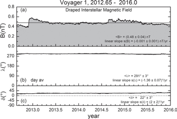
Figure 1. Draped interstellar magnetic field observed by V1 from 2012.65 to 2016.0. This figure shows the magnetic field strength B (a), the azimuthal angle λ (b), and the elevation angle δ (c), respectively, in RTN coordinates.
Download figure:
Standard image High-resolution imageThe average magnitude of  shown in Figure 1(a) is
  nT, which is significantly stronger than the magnetic fields previously observed anywhere in the heliosheath. Whang (2010) predicted that the magnitude of the draped interstellar magnetic field at the nose of the heliopause would be approximately 1.7 times that of the undisturbed interstellar magnetic field, in which case the observations imply an upper limit of the interstellar magnetic field Bist ≤ 0.3 nT or 3 μG. Isenberg et al. (2015) published another analytic model of draping and discussed its relationship to Voyager observations and the IBEX ribbon.
The average azimuthal angle in Figure 1 is  and the average elevation angle is
  . These angles are close to the Parker spiral magnetic field direction (Parker 1958) at the position of V1 (λ = 270°, δ = 0°), but the difference is significant, as discussed by Burlaga & Ness (2014a). Voyager 1 was measuring the draped interstellar magnetic field during the interval shown in Figure 1. The direction of this magnetic field is close to the −T direction, pointing from west to east when looking from Voyager 1 to the Sun, and the positive δ indicates that the draped interstellar magnetic field is pointing northward relative to the solar equatorial plane. A linear fit to the elevation angle as a function of time gives a slope s(δ) = (2 ± 2)° yr−1, and a similar fit to the azimuthal angle as a function of time gives a slope s(λ) = (−1.36 ± .07)° yr−1 as shown in Figure 1. Earlier fits by Burlaga & Ness (2014b) during the shorter interval between 2013.00 and 2014.41, found
  and
and  , respectively; this is consistent with the latest data, but the angles λ and δ varied linearly with a slope s = (1.4 ± 0.1)° yr−1, which has a sign opposite to that observed in the larger interval. The difference in these results can be attributed to the much longer interval now under consideration. The systematic errors, which are discussed below, were not considered in the mathematical uncertainties associated with the linear fits. The model of Usmanov et al. (2016) and Isenberg et al. (2015) predicted a linear decrease in δ and a linear increase in λ throughout the outer heliosheath with the scale of the order of 150 au or more.
The small difference between the Parker spiral direction and the direction of the heliosheath magnetic field observed by V1 was initially surprising. However, a re-examination of the results of Pogorelov et al. (2013), plotting angles instead of components of  , showed that they actually predicted that the angle between the draped interstellar magnetic field in the heliosheath fields should be δ ≈ 25° and λ ≈ 290°, consistent with the observations shown in Figure 1, within the uncertainties of the observations. The simulations of Pogorelov et al. (2013) and Borovikov et al. (2012) do not support the idea of Opher & Drake (2013) that the ISMF vector becomes nearly parallel to the solar equatorial plane, regardless of its direction in the unperturbed local interstellar medium (LISM).
Zirnstein et al. (2016) used IBEX observations to show that draping of the ISMF around the heliopause can be used to precisely determine the magnitude (2.93 μG ± 0.08 μG) and direction (22728 ± 069, 3462 ± 045 in ecliptic longitude and latitude, respectively) of the pristine ISMF far (∼1000 au) from the Sun. They found that the ISMF vector is offset from the ribbon center by ∼83 toward the direction of motion of the heliosphere through the LISM, and that their vectors form a plane that is consistent with the direction of deflected interstellar neutral hydrogen. Their results yield draped ISMF properties close to the magnetic field observed by V1 above, and they give predictions of the pristine ISMF.
3. MAGNETICALLY DISTURBED AND QUIET INTERVALS
Figure 1 shows that there were two intervals with small (<20%) but significant enhancements in B between 2012.65 and 2016.0. These enhancements can be seen more clearly in Figure 2, which has the same data as Figure 1, plotted with smaller ranges for the ordinates. Five distinct intervals labeled 1 through 5 are shown in Figure 2. During Interval 1, a relatively weak B decreased from 2012.65 to 2012.9. A disturbed interval (Interval 2), beginning with a shock and containing relatively strong magnetic fields, was observed from 2014.91 to 2013.36. A relatively undisturbed interval (Interval 3) extended from 2013.36 to 2014.64. The new observations, from 2014.74 to 2016.0, include Interval 4 containing strong magnetic fields extending from 2014.6 to 2015.4 and the relatively quiet Interval 5 from 2014.4 to 2016.0.

Figure 2. V1 observations of the magnetic field from 2012.65 to 2016.0. These are the same data that are shown in Figure 1, but the range of the ordinate in each panel is restricted in order to exhibit the structure of the small changes in the magnetic field. Five distinct regions are identified in the top panel, labeled 1 through 5.
Download figure:
Standard image High-resolution image4. DECREASING MAGNETIC FIELD STRENGTH JUST BEYOND THE HELIOPAUSE
During Interval 1, B was relatively weak compared with the average value  nT from 2012.65 to 2016.0, and it declined from 0.44 nT to 0.39 nT. The azimuthal direction λ of
  during this interval increased linearly from 286° to 295° and the elevation angle δ changed from 16° to 20°. Thus, the average values of λ and δ during Interval 1 are 291° and 18°, respectively, which are consistent with the average values for the entire interval in Figure 1, λ = 291° ± 3 and δ = 22° ± 3°. In other words, the average magnetic field direction during Interval 1 is consistent with our identification of
  as the draped interstellar magnetic field for the entire interval shown in Figure 1.
The reason for the relatively weak, declining B is not fully understood. Its appearance just after the last of the changes in the intensity of energetic particles (which is generally regarded as the outer edge of the heliopause) might be related to a "plasma depletion layer." The signature of the depletion layer on the sunward side of Earth's magnetopause is a decrease in B and an increase in the density and temperature from the boundary of the object (e.g., the magnetopause) to a distance upstream of Earth of the order of half the distance to the Earth's bow shock.
Fuselier & Cairns (2013) suggested a plasma depletion layer exists adjacent to the heliopause in the outer heliosheath as a result of draping of the interstellar magnetic field around the heliopause. A plasma depletion layer was first observed in the magnetosheath of the Earth, close to the magnetopause, in a region ≈0.3 RE thick in the sunward direction (Zwan & Wolf 1976; Erkaev 1988). A plasma depletion layer has also been observed in the sheath ahead of magnetic clouds propagating away from the Sun (Farrugia et al. 1995, 1997). In both cases, the cause of the plasma depletion layer is draping of the magnetic field around the obstacle, produced by its motion relative to the ambient medium.
Based on remote radio wave observations from Voyager, Gurnett et al. (1993) suggested that a ramp of increasing density exists in the interstellar medium just ahead of the heliopause. Gurnett et al. (2013) showed that (V1) observed electron plasma oscillations from 2013/99 to 2013/142 at a frequency of 2.6 kHz, corresponding to a very high electron density of 0.08 cm−3. They also noted an earlier electron plasma oscillations event at 2.2 kHz in 2012 October–November corresponding to a density of 0.05 cm−3. Because such densities are characteristic of interstellar plasma and are at least 50 times larger than those observed in heliosheath plasma by Voyager 2 (Richardson & Wang 2012), Gurnett et al. (2013) concluded that V1 was immersed in the interstellar plasma. They suggested that the increase in density from 0.05 cm−3 to 0.08 cm−3, from the time of the first burst of electron plasma oscillations to the second burst, is an indication of a density ramp, like that inferred by Gurnett et al. (1993) from remote observations of radio waves by V1, which were assumed to be radio waves generated by a shock of solar origin in interstellar plasma just beyond the heliopause.
Models 1 and 2 in Figure 4 of Zank et al. (2013), corresponding to an interstellar magnetic field equal to 2 μG and 3 μG respectively (for which a bow wave exists), produce densities increasing from 0.05 cm−3 to 0.1 cm−3 in the interstellar plasma near the heliopause, consistent with the observations of Gurnett et al. (2015) and increasing density extending far into the outer heliosheath. Since the density ramp predicted by Zank et al. and that observed by Gurnett et al. extend well beyond Interval 1, where it is not associated with an observed increase in B, its relationship to a plasma depletion region is in doubt. However, a recent model by N. V. Pogorelov et al. (private communication, 2016) does show an increase in density and a decrease in B, with increasing distance from the heliopause.
5. COMPARISON OF THE DISTURBED INTERVALS 2 AND 4
Both Interval 2 and Interval 4 began with a step-like increase in B. Interval 4 began with a 20% jump in B centered on 2014/236 (2014.6483), and Interval 2 began with a 7% increase in B centered at 2012/335 (2012.9153). We shall refer to these jumps as weak "shocks" based on the evidence in Section 5.1, but we cannot rule out the possibility that they are simply compression waves. In both intervals, B remained higher than average for months following the jump in B, and each interval ended with a relatively abrupt decrease in B. During Interval 4, V1 observed quasi-periodic oscillations with a period approximately that of the solar rotation. Such oscillations were not seen during Interval 2.
5.1. Shocks in Interval 2 and Interval 4
The shocks at the beginning of Interval 2 and Interval 4 are illustrated in Figure 3. Both shocks were preceded by an interval containing electron plasma oscillations, which ended abruptly when the shock arrived (Gurnett et al. 2013, 2015, respectively). The presence of these electron plasma oscillations supports the interpretation of the jumps in B as shocks, as it is known that electron plasma oscillations can be produced by a beam of electrons accelerated by a shock (Filbert & Kellogg 1979; Scarf et al. 1979, 1971).
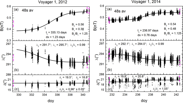
Figure 3. 48 s averages of B observed by V1 during the intervals from 2012, day 329 to 241, (left panel) and from 2014, day 229 to 243 (right panel).
Download figure:
Standard image High-resolution imageWe fit the magnetic field strength profiles B(t) in Figure 3 to the sigmoidal (Boltzmann) curve B(t) = B2 + (B1 − B2)/(1 + exp [(t − to)/τ)] (where B1 and B2 are the magnetic field strength before and after the jump, t is the time in days, and to is the center time of the symmetric distribution). A fit of B(t) for the 2012 shock shown in the left panel of Figure 3(a) gives an excellent fit with the parameters B1 = 0.38 nT, B2 = 0.56 nT, to = 335.13 days, and τ = dx = 1.23 days. The time τ is a measure of the passage time of the shock; 80% of the change in B occurs within a time w = 4.4 τ (see, e.g., Burlaga et al. 2011, where it is also shown that the Boltzman curve is related to the arctangent function).
An inspection of Figure 3 shows that both shocks were "laminar", i.e., the transition across of B each shock was smooth, lacking any features or waves except the noise that was produced by the instrument (±0.003 nT) and the digitization error (±0.004 nT). This is a feature associated with a "subcritical resistive laminar shock" at 1 au (Kennel et al. 1985; Mellott 1985). The magnetic field in the two outer heliosheath shocks are quite unlike the highly structured and variable magnetic fields observed at the termination shock by V2 (Burlaga et al. 2008).
The jump in B across the 2014 shock was B2/B1 = 1.13. The electron density average before and after the shock was 0.0873 and 0.0968 cm−3, respectively (Gurnett et al. 2015), which gives a density ratio of =1.11. The ratios B2/B1 and N2/N1 are essentially the same within the uncertainties, consistent with the prediction for a perpendicular shock, B2/B1 = N2/N1.
In comparison, the shock observed in the interstellar magnetic field on day 2012/335.43 had a jump B2/B1 = 1.5, which is larger than that observed on 2014/day 236 (B2/B1 = 1.1), but it was still a weak shock (Burlaga et al. 2013). There was little change in the magnetic field direction, consistent with a perpendicular shock.
The shock normal can be estimated from the magnetic field observations alone using the co-planarity theorem (Colburn & Sonett 1966). The uncertainties are large because there was only a small change in direction across the shock, as may be seen in Figure 2. The RTN components of B before and after the 2014 shock were  nT and
  nT, respectively. The shock normal was
  , and the corresponding angle between the shock normal and the radial direction was 16°, indicating that the shock was propagating nearly radially. The angle between
  and
and  was 61° consistent with a quasi-perpendicular shock. For the 2012 shock, the shock normal was
  , the angle between
  and the radial direction was 28°, and the angle between
  and
and  was 85° consistent with a quasi-perpendicular shock.
The minimum speed of the shock relative to the upstream flow must be greater than the magnetoacoustic speed, which is  . The adiabatic sound speed in the medium upstream of the shock, depends on the temperature upstream of the shock, which we take as 20,000° K just beyond the heliopause (Zank et al. 2013), which gives VS1 = 17 km s−1. For the 2014 shock, the Alfvén speed was
  where mp is the proton mass, B1 = 0.48 nT, and N1 = 0.087 cm−3, which gives VA1 = 36 km s−1. Consequently, the magnetoacoustic speed was VMA = 39 km s−1, and the 2014 shock must have been moving faster than this. At 1 au, a subcritical shock has a magnetoacoustic Mach number less than ≈2. Thus, the 2014 shock was probably propagating at a speed ≤80 km s−1 relative to the upstream medium. For the 2012 shock, Burlaga et al. (2013) obtained VA1 = 38 km s−1 and chose the same sound speed VS1 = 17 km s−1, giving the magnetoacoustic speed VMA = 42 km s−1.
Another important parameter is the ratio (VA1/VS1)2, which is equal to 4.5 for the 2014 shock and 4.9 for the 2012 shock. Thus, for both shocks (VA1/VS1)2 ≫ 1 and VA1 > VS1, consistent with a subcritical resistive shock (Kennel et al. 1985) at 1 au. However, the effect of nonthermal ions and neutral particles should be considered in the outer heliosheath.
Let us now consider the shock thickness. Since the Boltzman fit to B(t) for the 2014 shock in Figure 2 gives τ = 0.76 days, the width (or transit time) of the jump is w = 3.3 days. Thus, the shock moved past V1 during an interval of the order of 2 × 10⁵ s. We will assume that the interstellar plasma is approaching the Sun at a speed of 3 km s−1 at the position that V1 (Krimigis et al. 2011). Assume that the weak shock moved at Mach 1.5, ≈60 km s−1, relative to an approaching observer in the frame of the upstream medium. Since V1 is moving away from the Sun at 17 km s−1 relative to the Sun, it was moving at 20 km s−1 relative to the upstream medium in 2014. Thus, the speed of the shock relative to V1 was ≈40 km s−1. The V1 observations show that the shock moved past V1 during an interval of ≈2 × 10⁵ s. Thus, the shock thickness was ≈107 km. Since the ion inertial length in the plasma was ωpi = 800 km s−1, the 2014 shock thickness was ≈104 c/ωpi. The 2012 shock thickness was also ≈104 c/ωpi (Burlaga et al. 2013).
The thickness of the ramp of the supercritical termination shock TS-3 observed by V2 was of the order of 6000 km ≈1 c/ωπ, and the thickness of the ramp and overshoot combined to make a shock thickness of the order of 25 c/ωpi (Burlaga et al. 2008). The thickness of a laminar subcritical resistive shock at 1 au is ≈3 c/ωpi (Greenstadt et al. 1975). It is not clear why the shocks in the outer heliosheath are ≈3000 times thicker than the subcritical resistive shocks observed in the solar wind at 1 au and ≈500 times thicker than the supercritical termination shock. The dominance of nonthermal pickup protons in the interstellar plasma in the outer heliosheath must be an important factor in determining a shock thickness, but to our knowledge there is no systematic study of the structure of shocks in the outer heliosheath.
5.2. Origin of the Shocks and Post-shock Magnetic Fields
Information about the origin and detailed nature of the individual disturbances (CME's, and magnetic clouds, and corotating streams) cannot be derived from the distant Voyager observations, because memory of the disturbances is lost as a result of interactions among the flows within several au of the Sun (Burlaga et al. 1983). However, when systems of transient and corotating flows are observed for 1–3 solar rotations at 1 au, the flow systems carry magnetic fields and momentum from the Sun. Although individual flow profiles are lost, the flows and magnetic fields can combine to form a large region with relatively strong magnetic fields, a Global Merged Interaction Region, (GMIR), with a radial dimension ≈20 au which encircles the Sun and extends to high latitudes (Burlaga et al. 1984). The individual shocks produced by transient flows from the Sun can overtake one another and merge to form stronger shocks. These shocks can merge with the corotating shocks associated with corotating streams within 10 au tending to form even stronger shocks, offsetting the decrease in shock strength associated with increasing distance from the Sun (Burlaga 1995). Thus, a large GMIR, often preceded by a shock, forms beyond 20 au (Burlaga et al. 1984, 1993; Whang et al. 1999; Pogorelov et al. 2012) and can interact with the termination shock (Burlaga & Whang 1999). The radial evolution of the GMIR has been modeled by Burlaga et al. (2013). A GMIR, possibly preceded by a shock, has been observed within the heliosheath during 2006 by Voyager 2 (Burlaga et al. 2011). The strong magnetic fields in this GMIR, as in most GMIRs, produced a depression in the cosmic ray counting rate, after which the cosmic ray intensity recovered in about 200 days, giving a long-lasting Forbush decrease.
Gurnett et al. (1993) observed radio waves with the instrument on V1 which they proposed were produced by a GMIR propagating at ≈40 km s−1 in a region just beyond the heliopause, within the outer heliosheath, whose shock moved past the heliopause and generated radio waves in interstellar plasma. This kind of interaction may be the cause of the shock bounding Interval 2. Assuming spherical symmetry, Whang & Burlaga (1994) calculated the evolution of a "GMIR shock" originating in the supersonic solar wind as a result of merging of coronal mass ejections and other flows produced by the Sun. In their model, two shocks are produced by the GMIR shock when it collides with the heliopause (treated as a tangential discontinuity). One shock moves away from the Sun into the outer heliosheath, and the other shock moves toward the Sun through the inner heliosheath. Such shocks were described in more detail by the global time-dependent models of Zank & Müller (2003), and Washimi et al. (2011, 2015), who found that they were weak shocks. Thus, the hypothesis of Gurnett et al. (1993) that heliospheric shocks can propagate through the heliopause into the interstellar plasma is supported by all of these theoretical models.
Pogorelov & Zank (2005) developed a 3D model that follows a GMIR-like perturbation through the termination shock and into the heliosheath, but not beyond the heliopause. Pogorelov et al. (2012) extended their 3D time-dependent model to follow the evolution of the flows and magnetic fields past the heliopause and into the outer heliosheath. Figure 18 in the review by Zank (2015), from the paper of Washimi et al. (2011), shows clearly how a series of magnetic pressure pulses can be transmitted through the heliopause and propagate to at least 25 au into the outer heliosheath, where they appear to broader and in some cases overlap.
Liu et al. (2014) used solar observations and observations made near 1 au as input to a 1D MHD model to compute the evolution of a cluster of shocks and interplanetary CMEs out past the termination shock, through the inner heliosheath, pass the heliopause, and into the outer heliosheath. Their model predicts a formation of a large merged interaction region with a preceding shock that would reach 120 au near 2013/April 22, which coincides with the observation of radio emissions (Gurnett et al. 2013) and a transient disturbance in the galactic cosmic rays detected by V1. Unfortunately, they did not plot the profiles of B as a function of distance. Fermo et al. (2015), using a 1D time-dependent MHD model, followed the evolution of a GMIR past the heliopause and into the outer heliosheath, showing both the magnetic field disturbance produced by the shock and magnetic disturbances behind it, although the resolution of the calculation was relatively low. Clearly, the next generation of models together with realistic input conditions and the constraints imposed by Voyager observations will be capable of producing a realistic description and deeper understanding of the structure and dynamics of the outer heliosheath.
During Interval 2, the relatively strong magnetic fields following the shock decreased monotonically for 123 days, with small random fluctuation superimposed, as shown in Figure 3. One might expect this simple profile to be observed in a small region following the shock, but it is not clear why it persisted for 123 days, when various types of magnetized flows were ejected by the Sun.
During Interval 4, the relatively strong fields following the shock decreased in a more complex and interesting way for 267 days as shown by careful examination of Figure 3. The variation can be resolved into two components as shown in Figure 4(a): (1) a linear decrease of B with increasing time and (2) a quasi-sinusoidal variation of the difference between B and the linear fit shown in Figure 4(b). The linear decrease occurred between 2014.8330 and 2015.3700. A sine wave with a constant amplitude and a constant period was fit to the observations of B in Figure 4(b), and the period was found to be 28 days. Since the sine wave describes seven of the eight maxima in B that were observed during this interval, we may say that the fluctuations were quasi-periodic with a period of ≈28 days, which is close to the solar rotation period in the spacecraft frame. This is a strong indication that the fluctuations in B observed during Interval 4 were produced by solar/solar wind related disturbances. However, such fluctuations in the outer heliosheath were not predicted, and the mechanism that produces these fluctuations is not known. Thus, the observations of strong, quasi-periodic magnetic fields during Interval 4 pose a problem for the theorists, which can be investigated with the next generation of models.

Figure 4. Observations of the B from 2014.8330 to 2015.3790 show two components: a linear decrease in B (a) and quasi-periodic oscillations within a period of 28 days.
Download figure:
Standard image High-resolution image5.3. The Boundaries at the End of Interval 1 and Interval 4
As shown in Figure 2, Interval 2 ended rather abruptly with a decrease in B on 2013/130 (2013.3534) after the shock on 2012/335, and Interval 4 ended abruptly with a decrease in  on 2015/236.71, after the shock on 2014/236. Thus, the relatively strong magnetic fields during Interval 2 compared to the average magnetic field in the outer heliosheath were observed for ≈163 days, and the relatively strong magnetic fields during Interval 4 were observed for ≈267 days.
As discussed above and shown by the vertical dashed lines in Figure 2, Interval 2 and Interval 4 ended rather abruptly, just as they began. The quantitative structure of the abrupt decreases in  at the end of these intervals is shown in the two panels of Figure 5, which plot hour-averages of B, λ, and δ for brief intervals during 2013 and 2014, respectively. As in Figure 2, the observations are magnified by plotting the magnetic field strength and direction over limited ranges of the ordinates in the two panels in Figure 5. The same ranges for the ordinates are used in both panels, so that the observed changes can be compared directly. However, the abscissa for the 2015 data extends over a broader interval than that the 2013 data.
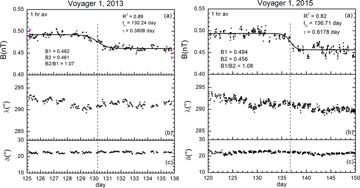
Figure 5. Abrupt decreases in B at the end of Interval 2 (left panel) and at the end of Interval 4 (right panel). The format of each panel is the same as that in Figure 3.
Download figure:
Standard image High-resolution imageThe magnetic field strength decreased smoothly between two intervals with nearly constant B for both the 2013 and 2015 Voyager observations, as shown in the two panels in Figure 5. The magnetic field strength profiles are fitted accurately with a Boltzman function (which is equivalent to an arctangent curve), as we found for the fits to the fast forward shocks. The quality of the fit was R2 = 0.89 and R2 = 0.82 for the 2013 and 2015 events, respectively. For the 2013 event, which was centered at to = 2013/130.24, the jump in B was a decrease from B1 = 0.492 nT to 0.461 nT giving B1/B2 = 1.07. For the 2015 event, which was centered at to = 2015/136.71, the jump in B was from B1 = 0.494 to 0.456 nT giving B1/B2 = 1.08. Thus, the two profiles are very similar in form and magnitude. The main difference between the two profiles is in the passage time, which was w = 4.4 τ = 1.68 days for the 2013 event and 2.72 days for the 2015 event. These passage times are similar to the corresponding passage times for the shock waves discussed above, namely, 5.41 days and 3.34 days for the 2012 and 2014 shocks at the beginning of Interval 2 and Interval 4, respectively.
The similarity in the shapes of the abrupt decreases in B shown in Figure 5 and the shapes of the "shocks" associated with electron plasma oscillations in Figure 2 is significant, and we must consider the physical significance of the profiles. The discussion in the preceding section presents strong, but not conclusive evidence that the structures in Figure 2 are forward shocks. However, we cannot discount the possibility that they are non-dissipative pressure waves, at least at the locations and times at which they were observed. The similarity of the passage times and jumps in B for the abrupt decreases in B shown in Figure 5 and the shocks in Figure 3 suggest the possibility that the abrupt decreases in B are reverse shocks. The fact that the passage time of the abrupt decreases in B is shorter than the passage time of the fast shocks is consistent with the reverse shock hypothesis, but it is not sufficient to identify them as reverse shocks.
Another possibility is that the abrupt decreases in B are stationary current sheets associated with tangential discontinuities embedded in the interstellar plasma that is carrying the current sheets toward the Sun and past V1. Boltzman profiles for abrupt changes in B have been observed quite generally (Burlaga & Ness 2011) for tangential discontinuities associated with pressure balanced structures (PBS) (Lemaire & Burlaga 1976), which are stable equilibrium current sheets advected with the flow.
Assume that the interstellar plasma is approaching the Sun at a speed of 3 km s−1 in the outer heliosheath at the position of V1. Since V1 is moving away from the Sun at 17 km s−1 relative to the Sun, the current sheets moved at 20 km s−1 relative to V1. Since the passage times for the abrupt decreases in B were 1.7 days for the 2013 event and 2.7 days for the 2015 event, the corresponding thicknesses of the current sheets were 2.9 × 10⁶ km and 4.7 × 10⁶ km for the 2013 and 2015 event, respectively. Since the thermal proton gyroradius (Larmor radius) computed assuming the temperature of 20,000° K was RL = 4 × 10⁶ km, the thickness of the current sheets were 0.7 RL, and 1.2 RL, which are close to the current sheet scale 2–10 RL predicted by Lemaire & Burlaga (1976) in their analysis of current sheets associated with PBS. These length scales are smaller than the length scale (≈15 RL) of current sheets observed in the inner heliosheath by Burlaga et al. (2011). However, in view of the fact that the flow speed of the plasma and the temperature of the plasma in the outer heliosheath near V1 are estimates rather than observations, we can conclude that the abrupt decreases in B at the end of Interval 2 and Interval 4 are consistent with current sheets associated with MHD tangential discontinuities.
6. COMPARISON OF THE RELATIVELY QUIET INTERVALS 3 AND 5
Voyager 1 observed a 468 day interval (Interval 3) from 2013.3616 (2013/133) to 2014.6410 (2014/235) in which B was relatively uniform and close to the average magnetic field value, which is shown in Figure 2. Burlaga et al. (2015) suggested that this interval might be relatively undisturbed by solar/solar wind perturbations, and they showed that the small amplitude fluctuations in B in the outer heliosheath had a Kolmogorov spectrum, which could be identified as the spectrum of the draped interstellar magnetic field with an outer scale of the order of 1 pc. A sample of the fluctuations in this interval is shown by the points corresponding to the difference between daily averages of B and a linear least squares fit B, which are plotted in Figure 6(b). Because the amplitude of the fluctuations was very small (<0.02 nT), which is to be compared to the noise level and digitization level of the instrument, 0.005 nT), the noise was filtered out by a 9-point Savitzsky–Goulet filter, giving the solid curve in Figure 6(b).

Figure 6. Daily averages of B (dots) and a curve (solid) constructed using a 9-point Savitzsky–Goulet filter showing fluctuations observed during Interval 5 (a) and the corresponding results for a sample of the turbulence observed during 2013.
Download figure:
Standard image High-resolution image
More recently, V1 observed another quiet interval that extends from 2015.4000 (2015/147) through 2016.0 (2015/365) (Interval 5 in Figure 2), which might also be representative of the draped interstellar magnetic field, relatively undisturbed by the Sun. The data in this interval are shown more clearly in the bottom panel of Figure 2, in which the fluctuations in B are exaggerated for clarity by changes in the scales. The differences between the daily averages of B and the corresponding values of B from a linear least squares fit to these observations during Interval 5 are shown the points in Figure 6(a). The corresponding 9-point Savitzsky–Goulet filtered data are shown by the smooth curve in Figure 6(a). (A discussion of the Savitzsky–Goulet filter may be found at https://en.wikipedia.org/wiki/Savitzky%E2%80%93Golay_filter). The amplitude and appearance of the two curves in Figure 6 are very similar, suggesting that Interval 3 and Interval 5 might represent a similar state of the draped interstellar magnetic field.
Figure 2 shows that λ increased nearly linearly from 291° to 295° with time throughout Interval 3. Since the statistical uncertainty in the angles is at least ±2° and the systematic errors could be larger, one must be very cautious in interpreting this change in direction of only 4°. The change in the elevation angle δ was even smaller. Schwadron et al. (2015) expressed these angles in heliocentric (J 2000) ecliptic coordinates and extrapolated these observations linearly to large distances. They found that the extrapolated magnetic field direction passes through the center of the IBEX ribbon, at ecliptic longitude ∼220° and ecliptic latitude ∼40°, consistent with the view that that the center of the IBEX ribbon defines the direction of the LISM.
Interval 5 in Figure 2 is a relatively undisturbed interval, similar to Interval 3, with even weaker average magnetic fields, and one might expect to observe temporal variations in λ and δ similar to those observed during Interval 3. However the variation of λ and δ in Interval 5 is very different, qualitatively and quantitatively, than that in Interval 3. It is possible that the systematic errors happened to be greater in Interval 5, although there is no way to demonstrate this. It is also possible that Interval 5 is not representative of the relatively undisturbed magnetic field. The latter possibility is supported by the observation of electron plasma oscillations in the middle of Interval 5 (Gurnett et al. 2015). These electron plasma oscillations were presumably produced by energetic electrons accelerated by a shock. No shock was observed by V1 in this case, but it might have been present in region of the outer heliosheath that was not sampled by V1. Continued observations during 2016 might clarify the nature of the magnetic field during the extension of Interval 5.
7. SUMMARY AND DISCUSSION
Since 2012 August 25, the magnetometers on V1 have been observing the draped local interstellar magnetic field (LISM) in the outer heliosheath. The interstellar magnetic fields in the outer heliosheath are distinctly different from the magnetic fields previously observed in the inner heliosheath, which is generally referred to as the "heliosheath" in the literature. In the inner heliosheath the B is relatively weak (0.1 nT) with a highly variable multifractal structure, a magnetic field direction that is distributed bi-modally about the Parker spiral angles, as well as sectors and sector boundaries. In the outer heliosheath the average B is relatively strong (0.48 nT), and a linear least squares fit to B gives an average slope of (0.001 ± 0.001) nT yr−1, indicating that B does not change significantly on a scale of 3.4 years, during which V1 moved nearly 11 au. Similarly, the average direction of  during this 3.4 year interval was nearly constant with
  and
and  , with no significant net change across the interval. During the past three years the B fluctuated by <20% about the average B, while the magnetic field direction was remarkably constant, changing nearly monotonically by less than several degrees in any interval observed to date.
Models of the outer heliosheath indicate that its extent in the upstream direction is ∼100 au or more (e.g., Usmanov 2016; Zank 2015) compared to the region sampled by V1. Thus, V1 has observed only about 10% of the upstream outer heliosheath, and it may never observe more than ∼30% of this region.
Just after permanently crossing into the outer heliosheath, V1 observed a small but significant decline in the B, which is still not understood. Although it has been suggested that this interval represents a plasma depletion layer, we present evidence which does not support this hypothesis.
We identified a new interval (Interval 4) beginning with a weak shock, followed by stronger magnetic fields that decreased behind the shock and contained ∼28 day oscillations in B, which suggests that the Sun was influencing this region. Previously a similar region, Interval 2, was observed beginning with a weak shock and followed by stronger magnetic fields that decreased with time to the mean value of B, but with no 28 day oscillations. The nature and origin of the strong fields following the shocks in Interval 2 and Interval 4 and the cause of the 28 day oscillations are not understood
The shocks preceding Interval 2 and Interval 4 were very similar, being weak quasi-perpendicular shocks with B2/B1 = 1.1 and 1.4 respectively, and with a thickness of the order of 104 ion inertial lengths. The large thickness of these outer heliosheath shocks compared to those observed at 1 au is not understood. The azimuthal angle of  appeared to decrease nearly linearly with increasing time during Interval 4, although it is difficult to separate this observation from the systematic errors in the data.
Interval 4 and Interval 2 ended with an abrupt decrease in B. We found that this boundary has a structure consistent with that of a current sheet (a PBS) across which B decreased by 8% and the direction of  did not change. The thickness of the current sheets at the rear boundary of Interval 4 and Interval 2 was 0.7 RL, and 1.2 RL, based on an estimated temperature used to compute RL. Theoretically, the thickness of a PBS is 2–10 RL where RL is the Larmor radius. The thickness of current sheets observed in the inner heliosheath is ≈15 RL.
These estimates of the thicknesses of the current sheets are all consistent with one another given the uncertainties in the geometry, speed, and temperature used determined the thicknesses and RL. On the other hand, we emphasize that the thickness of the current sheets at the end of Interval 2 and Interval 4 are comparable to the thicknesses of the forward shocks at the beginning of Interval 2 and Interval 4. Thus, we cannot exclude the possibility that these current sheets were actually reverse shocks or perhaps pressure wave.
We also identified a new interval (Interval 5) with relatively undisturbed magnetic fields. The magnetic field strength in this new interval contained small fluctuations in B (up to ±0.02 nT) which were similar to the fluctuations associated with the turbulence discussed by Burlaga et al. (2015) and shown in Interval 3. The azimuthal angle of  in Interval 3 increased linearly with time, while the elevation angle increased linearly at a much slower rate. Schwadron et al. (2015) showed that a linear extrapolation of direction of
  in Interval 3 would fall near the middle of the IBEX ribbon. However, a decrease in the azimuthal angle of
  was observed in the corresponding Interval 5. Moreover, electron plasma oscillations were observed in this interval, which were probably associated with a nearby shock that was not detected by the magnetometer on V1. The presence of these electron plasma oscillations suggest that this interval was also affected by the Sun, if only indirectly, by nearby solar/solar wind induced perturbations of the magnetic field in the outer heliosheath.
This study shows that even though V1 was observing the draped interstellar magnetic fields and interstellar plasma in the outer heliosheath from 2012 to 2016.0 August 15, the Sun and solar wind were significantly perturbing this medium during two extended intervals. This conclusion is consistent with earlier studies showing that heliospheric shocks can interact with the heliopause and produce reflected shocks which propagated back into the inner heliosheath as well as transmitted shocks which propagated into the outer heliosheath.
Our results also reveal new phenomena in the outer heliosheath, discussed above, and they demonstrate the need for more detailed theoretical and observational studies of (1) the nature, thickness and propagation of shocks throughout the outer heliosheath, (2) the propagation of other kinds of disturbances within the outer heliosheath, (3) the origin of strong fields behind the shocks, which persist for more than 100 days, (4) the possibility that heliosheath material may occasionally be observed as a result of an instability that modifies the structure and nature of the heliopause, (5) the radial extent of the solar wind induced perturbations and (6) the effect of solar cycle variations in the structure and dynamics of the outer heliosheath. Continued observations of the outer heliosheath by both V1 and V2 are very important, since this is a large unexplored region which is the final transition to the interstellar medium. However, it will be increasingly difficult to make the measurements, owing to the decreasing power available to operate the spacecraft and the experiments, as the Voyager spacecraft approach the end of their ability to function.
T. McClanahan, S. Kramer, and Robert Candey provided support in the processing of the data. D. Berdichevsky computed correction tables for the three sensors on each of the two magnetometers. N.F. Ness was supported by NASA grant NNX12A63G3G to the Catholic University of America. L.F. Burlaga was supported by NASA contract NNG14PN24P.