ABSTRACT
The interaction of an intergranular downdraft with an embedded vertical magnetic field is examined. It is demonstrated that the downdraft may couple to small magnetic twists leading to an instability. The descending plasma exponentially amplifies the magnetic twists when it decelerates with depth due to increasing density. Most efficient amplification is found in the vicinity of the level, where the kinetic energy density of the downdraft reaches equipartition with the magnetic energy density. Continual extraction of energy from the decelerating plasma and growth in the total azimuthal energy occurs as a consequence of the wave-flow coupling along the downdraft. The presented mechanism may drive vortices and torsional motions that have been detected between granules and in simulations of magnetoconvection.
Export citation and abstract BibTeX RIS
1. INTRODUCTION
Millions of granules representing the visible tops of convective cells cover the photosphere of the Sun. They have different shapes and sizes. Hot material rising to the surface in bright granules falls back down along the cool and dark intergranular lanes. Numerical experiments show that the topology of convection beneath the solar surface is dominated by effects of stratification. This leads to gentle, expanding and structureless warm upflows on the one hand, and strong, converging filamentary cool downdrafts on the other hand (Stein & Nordlund 1989). These experiments are confirmed by spectral observations of granulation which reveal blue shifts in the bright sections with red shifts and increased line widths in the darker sections (Nesis et al. 2001).
The magnetic field is ubiquitously present in the solar photosphere and exhibits a wide range of scales and strengths (Solanki et al. 2006; de Wijn et al. 2009). Magnetic flux emergence through the solar surface is driven by buoyancy and advection. On granular scales, it undergoes continual deformation and displacement because the ratio of gas to magnetic pressure is large in the convection zone. Diverging upflows sweep magnetic flux to intergranular downflow lanes where the downflow speeds significantly exceed the upflow speeds (Tao et al. 1998; Thelen & Cattaneo 2000; Weiss et al. 2002; Vögler et al. 2005). This results in a magnetic field strength of a few hundred Gauss at the solar surface. Flux tubes emerging through the surface are produced either from emerging loops that then open up through the top or by concentration of magnetic flux by horizontal flows in the intergranular lanes. Far below the surface their field lines spread out in many different directions (Stein & Nordlund 2006).
Further intensification to kG strength may be driven by the mechanism of convective collapse (Webb & Roberts 1978; Spruit & Zweibel 1979; Bushby et al. 2008). Numerical simulations of convective collapse (Danilovic et al. 2010) and Hinode/SOT observations (Nagata et al. 2008; Shimizu et al. 2008; Fischer et al. 2009) show downflows of between 7 and 14 km s−1.
Downdrafts are often seen to support vortices in simulations of convection (Muthsam et al. 2010) and magnetoconvection (Nordlund et al. 2009). Moll et al. (2011) found that the vortex features which develop in the downflow lanes typically exist for a few minutes, during which they are moved and twisted by the motion of the ambient plasma. Shelyag et al. (2013) argued that the apparent vortex-like motions are signatures of propagating twists or torsional Alfvénic perturbations rather than vortices.
Vortex flows were only recently detected in SST (Swedish Solar Telescope) and Sunrise observations of magnetic bright points in the photosphere (Bonet et al. 2008, 2010; Steiner et al. 2010). Photospheric twists and vortices are thought to be responsible for producing similar types of motions in the solar atmosphere. These include chromospheric swirls (Wedemeyer Rouppe van der Voort 2009), prominence tornadoes (Li et al. 2012; Wedemeyer et al. 2013), twists on spicules (De Pontieu et al. 2014). However, no clear connection has yet been established although some studies show that vortex tubes can penetrate into the chromosphere and substantially affect the structure and dynamics of the solar atmosphere (Kitiashvili et al. 2012a).
Different source terms in the vorticity equation have been considered as possible candidates for enhancement of vorticity in the solar context. Non-magnetic simulations of turbulent convection show that vortex stretching can be a primary source for the generation of small-scale vorticity (Kitiashvili et al. 2012b). The baroclinic term in the vorticity equation may lead to the formation of horizontally oriented vortex tubes (Steiner et al. 2010): the gradients of pressure and density are close to vertical in the convection zone, so their cross product is mainly horizontally oriented. During this process the vortex tubes move into the intergranular lanes and become vertical due to convective downdrafts. The generation of the vortical flows observed by Bonet et al. (2008) has been attributed to compression: the downdraft acts as a sink and as the matter has angular momentum with respect to the draining point, it must spin up when approaching the sink, giving rise to a whirlpool also known as the bathtub drainage effect (Spurk & Aksel 2008, p. 358).
The mechanisms described above are hydrodynamic in their nature. In the real Sun, interaction between vortices and ubiquitous magnetic fields is expected. Simulations of magnetoconvection usually begin with a weak, initially random (Moll et al. 2011) or uniform magnetic field (Stein & Nordlund 2006). Vortices with a small inclination appear mostly inside the integranular lanes where the downflows are strong. Horizontal flows advect the weak field and concentrate it in the turbulent downflow lanes where vortical motions are already well established.
One would expect stronger magnetic fields to have a stabilizing influence on the turbulent flows and vortex motions. However, Shelyag et al. (2011) found that when the field strength rises to a few kilogauss in the intergranular lanes, small-scale vortices and torsional motions develop at the photospheric level that are co-spatial with these magnetic field concentrations. These small-scale motions are not seen in the non-magnetic model. They demonstrated that the vorticity enhancement in the intergranular lanes was caused by a source term in the vorticity equation which contains magnetic tension.
Here, we describe how a downdraft may amplify twists of an ambient magnetic field. The theoretical mechanism behind the amplification process is the Alfvén instability introduced by Taroyan (2008). In the following sections, we present the model, the conditions under which twists may become amplified. In Section 3, we tackle the problem analytically to find the continuous spectrum of eigenvalues and construct the eigenfunctions. A forcing term is introduced in Section 4 and the governing equations are integrated numerically to examine the spatio-temporal evolution in the linear regime. In Section 5, the energy source and the physical nature of the instability associated with the twist amplification are discussed.
2. MODEL AND GOVERNING EQUATIONS
2.1. Downdraft Model
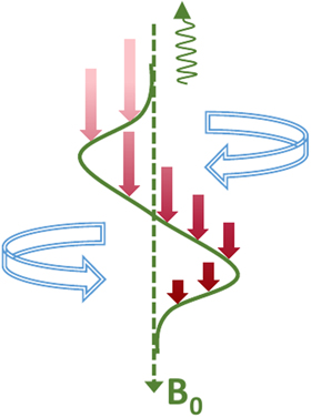
A near-vertical segment of an expanding magnetic flux tube is embedded in a gravitationally stratified convection zone and permeated by a field-aligned downdraft as shown in Figure 1. We assume that the plasma inside the tube remains in equilibrium with the surrounding medium.

Figure 1. Cartoon representation of an intergranular downdraft (red) in a near-vertical flux tube (green). The tube is in a horizontal pressure balance with the surrounding convection zone, where the density increases with depth due to gravitational stratification. The red vertical arrows become shorter and darker as the downdraft slows down in the lower dense regions. Twisting motions of the tube are indicated with blue arrows.
Download figure:
Standard image High-resolution imageThe density in the convection zone increases with depth due to the gravitational stratification. If the magnetic field remains constant then the density inside the tube will have to increase with depth as well in order to sustain a horizontal total pressure balance. According to mass conservation, the downdraft speed,  , where
  is the Alfvén speed defined as the ratio of the magnetic field and the square root of density with
  being the permeability of free space. Note that the flow speed decreases more rapidly with depth than the Alfvén speed does.
The critical level where  corresponds to equipartition between the magnetic energy density,
  , and the kinetic energy density of the flow,
  . The equipartition level may not exist if the magnetic energy dominates the kinetic energy of the downdraft everywhere in the upper subphotospheric layers.
We adopt a cylindrical coordinate system, where z denotes depth and θ represents the azimuthal coordinate. In the thin flux tube approximation, the linear equations governing the motion of small axisymmetric twists are decoupled from the other MHD equations. These motions are governed by the azimuthal components of the equations of momentum and induction (Hollweg et al. 1982; Ferriz-Mas et al. 1989):

where bθ, and vθ denote the azimuthal perturbations of the magnetic field and velocity, with

being the substantial derivative. Note that when θ is replaced by the Cartesian coordinate x, the same set of equations describes the propagation of shear Alfvén waves in a flowing plasma with a uniform magnetic field.
In the absence of an equilibrium flow ( ), the set of Equations (1) and (2) describes the propagation of incompressible Alfvén waves in a static medium. The waves result from the combined effects of the tension force (right-hand side of Equation (1)) and the plasma inertia (first term on the right-hand side of Equation (2)).
The presence of a constant flow ( ) leads to a constant Doppler shift due to the added advection term in the substantial derivative (3).
The last term on the right-hand side of the induction Equation (2) appears only when the equilibrium flow is variable. It represents the effects of compression or expansion of the plasma on the incompressible axisymmetric twists.
2.2. Twist Amplification: Analogy With Vortex Stretching
In a weak field, the Alfvén speed is small compared with the speed of the flow, and the inertial term in Equation (2) can be ignored. This eliminates the variable, vθ from the induction equation, so it can be rewritten as:

Therefore, expansion of the plasma ( ) corresponds to attenuation while compression (
 ) corresponds to amplification of bθ. From the preceding discussion it follows that the latter situation is more likely to occur in downdrafts.
Equation (4) looks remarkably similar to the vorticity equation for an incompressible fluid:

where ω denotes vorticity in the z direction. The right-hand side of Equation (5) represents the well-known vortex stretching effect: the angular velocity of a vortex tube increases when it is stretched and decreases when it is compressed (Spurk & Aksel 2008, p. 100).
In contrast, Equation (4) shows that the θ component of the magnetic field increases when the flow decelerates and decreases when it accelerates. The fact that the twist amplification stems from the induction equation emphasizes the magnetic nature of the process. Twist amplification may be thought of as a magnetic analogue of vortex stretching.
In a more general situation, when the magnetic field is not weak, the twist evolution requires a more detailed treatment. In the following sections we study the twist amplification analytically as an eigenvalue problem and numerically, and analytically. We also discuss the energy source, and the physics of the amplification process.
3. UNSTABLE TWISTS IN AN EXPONENTIALLY DECAYING DOWNDRAFT
The set of governing Equations (1) and (2) can be reduced to a single second order PDE for the magnetic field perturbation, bθ (Taroyan 2008):
where  , and
, and  . In deriving the above equation, we have used the equation of mass conservation. In a static medium with
  , the well-known wave equation can be derived from Equations (1) and (2):

Equation (7) was first analyzed by Ferraro (1954) in the context of Alfvén wave propagation in the solar atmosphere. Solutions in terms of the Bessel functions were constructed for an isothermal atmosphere with an exponential density profile:

where z0 is the scale height. The corresponding Alfvén speed is given by:

Note that in our notations z denotes depth. Equation (7) with the profile (8) was subsequently analyzed by different authors. They found standing wave solutions in terms of the Bessel functions (Ferraro 1954; An et al. 1989) or propagating wave solutions in terms of the Hankel functions (Hollweg 1978; Cally 2012) depending on the imposed boundary conditions.
An advantage of the smooth exponential profile is the absence of any model dependent artificial reflections that may arise due to discontinuities in the Alfvén speed or its derivatives (Cally 2012). One of the drawbacks is the finite Alfvén travel time to  (An et al. 1989).
In studies of the convection zone, it is common to adopt a polytrope with a linear temperature. Here, we adopt the exponential profiles (8) and (9) with a given scale height, z0. This approach allows us to compare our results with those already known from studies of Alfvén wave propagation in a stratified and static environment. Conservation of mass requires that the downdraft speed diminishes as:
provided the tube radius remains constant. We will see that the problems associated with the finite travel time to  are no longer relevant because the downdraft prevents propagation into the super-Alfvénic region.
The temperature represented by the square of the sound speed,  , can be determined from the equilibrium equation of motion:
where p0 is thermal pressure, g is the gravitational acceleration, and  is a general force term which vanishes at
  . Integration of Equation (11) yields:
where  , and
, and  is the limit of cs2 at
  . Thus, in contrast to a static force-free model, the sound speed is no longer a constant. Instead, the behavior of the sound speed and temperature will depend on the prescribed values for c0 and
  .
.
The coefficients in the governing Equation (6) are expressed through the Alfvén and flow speeds. Therefore, in the linear regime, the twist evolution does not depend on the temperature profile and the subsequent analysis is carried out without specifying the values of c0 and  .
.
Equation (6) is Fourier analyzed and the result is the following ODE:
where

The equipartition level where  represents a singularity in Equation (13). For simplicity we set this level at z = 0, so that
  . It separates the upper super-Alfvénic region,
  , from the lower sub-Alfvénic region,
  .
.
For small wavelengths,  , away from the singularity at z = 0, local phase speeds
  can be introduced. The plus sign corresponds to propagation in the positive direction. The minus sign represents propagation in the negative direction in the sub-Alfvénic region (
 ) and propagation in the positive direction when the flow is super-Alfvénic (
 ). Thus, in contrast to the static model, any perturbation in the super-Alfvénic region will be swept down into the sub-Alfvénic region without being able to reach
  .
.
We introduce a dimensionless variable:

so that,  and transform Equation (13) into:

where  , and
, and

The regular singularity at  corresponding to z = 0 requires separate treatment for
  (
( ) and
) and  (
( ).
).
We show in the appendix that the finite solution in the region  can be represented in terms of the modified Bessel function Kν:
where
and
with  . According to the definition (17) of ν, a positive value of
  corresponds to a positive value of
  , i.e., exponential growth in time. The growth rate is determined by the expression

Therefore, a finite solution to Equation (13) corresponds to an instability ( ). Note that solutions exist for arbitrary ν with positive
  and the spectrum of eigenvalues is continuous. It is well-known that if the coefficients of the differential equation are singular at the boundary or if the interval is infinite then the spectrum of eigenvalues is continuous and a Fourier integral replaces the linear combination of the eigenfunctions (Courant & Hilbert 1966, p. 340). In the present problem, the interval extends from z = 0 to
  and there is a singularity at z = 0.
The existence of the instability is not affected by the flow behavior in the region  . However, for completeness we construct the solution in the super-Alfvénic region assuming that the flow profile is determined by Equation (10). The finite solution in the region
  is expressed in terms of the Bessel functions
  (see appendix):

where


The coefficient C1 is derived assuming that vθ vanishes at  due to the super-Alfvénic flow.
Figure 2 displays  as a function of z and ν, where the normalization
  is applied. For simplicity, only real and positive values of ν corresponding to purely imaginary ω are considered. The corresponding eigenfunction shown in Figure 2 is also real. Note that the maximum of
  moves away from the equipartition level (z = 0) as ν increases.

Figure 2. Plot of  as a function of z and ν, where the normalization
  is applied. The color bar indicates the magnitude and the sign of
  . Only real and positive values of ν corresponding to purely imaginary ω and real
  are considered.
Download figure:
Standard image High-resolution imageOur analysis of the eigenvalue problem reveals the existence of an instability: small axisymmetric twists are exponentially amplified in a downdraft that exponentially decays with depth.
4. THE SPATIO-TEMPORAL EVOLUTION OF THE INSTABILITY
In this section, the evolution of a single twist is presented with two circumstances investigated. Both scenarios launch a single Alfvénic pulse from within the lower sub-Alfvénic part of the flux tube. However, the first case involves a static plasma with an exponential density profile (8), whereas the second case incorporates a downflow defined by Equation (10).
Equations (1) and (2) are numerically integrated using the flux-corrected transport scheme (Boris et al. 1993). A uniform grid is used which contains 1700 grid-points. The domain is extended in such a way that the boundaries are sufficiently far away from the region of interest as not to interfere with the simulations. The critical point where the flow changes from super-Alfvénic to sub-Alfvénic is situated at z = 0. The extension of the domain also means that any reflections or change in behavior of the perturbations is purely down to physical mechanisms, such as Alfvén speed variation, and is not a numerical implication caused from a boundary region.
In what follows, length, speed and magnetic field are normalized with respect to the scale length, z0, the Alfvén speed  , and the equilibrium magnetic field B0, respectively.
A smooth driver which describes a small-amplitude perturbation is added to the right-hand side of Equation (1) as a source term, F:
Here, A is amplitude, t is time normalized with respect to  , where
  and
and  are the start- and end-times for which the driver is active. Similarly,
  and
and  are the start- and end-points within the tube where the driver is active.
An exponentially decreasing profile is generated for the Alfvén speed (Figure 3: Top panel) with the plasma in a static equilibrium. A single twist is launched which separates into upward (negative direction) and downward (positive direction) propagating pulses (Figure 3: Middle and Bottom panels). The upward propagating pulse has an increasing amplitude in the velocity perturbation and a decreasing amplitude in the magnetic field perturbation. Note that the kinetic energy remains finite due to the density decrease with height. This behavior is well-known from studies of Alfvén wave propagation in stratified media (Cally 2012).
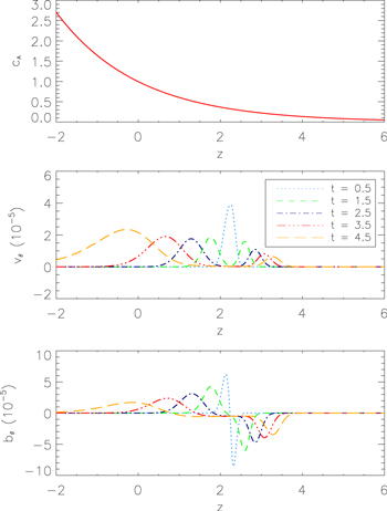
Figure 3. Top: Alfvén speed profile within a vertically stratified flux tube with no flow. Middle:  velocity distribution for time 0.5–4.5. Bottom: the corresponding
  profile.
Download figure:
Standard image High-resolution imageThe downward propagating pulse is impeded by the ever-diminishing Alfvén speed in the positive direction. The twist is not reflected due to the smooth equilibrium profile and its propagation comes to a virtual standstill until it is lost to the background plasma as the Alfvén speed approaches 0.
The introduction of a plasma flow yields some interesting results (Figure 4). The initial pulse is launched from within the flux tube and splits into two pulses that propagate in opposite directions, much like what is seen in the static case. The pulse that travels in the positive direction behaves identically to that seen in Figure 3. That is, the propagation of the pulse stalls with the  and
and  amplitudes decreasing until they are eventually lost to the background.

Figure 4. Top: Alfvén speed and flow-speed profiles within the modeled downdraft. The critical point  can be seen clearly at z = 0 where the two plots intersect one another. Middle:
  velocity distribution for time 0.5–8. Bottom: the corresponding
  profile.
Download figure:
Standard image High-resolution imageThe pulse that propagates upward in the negative direction behaves somewhat similarly to the pulse in Figure 3. However, unlike the static case, both bθ and vθ increase in amplitude as they propagate. As the pulse approaches the critical point, z = 0, the propagation virtually ceases with  and
and  continually amplifying (Figure 4: Middle and Bottom panels). This situation is allowed to arise due to the propagation speed
  gradually approaching 0. Using the expressions for the Alfvén and the flow speeds it can be shown that the travel time to z = 0,

is infinite. The pulse propagation does not extend to the super-Alfvénic region and the twist amplification is therefore unaffected by the flow profile in the region above the equipartition height. The pulse amplification in the vicinity of z = 0 confirms the instability found in the preceding section.
Figure 5 displays the twist evolution when the downdraft speed is much smaller than the Alfvén speed at z = 0. The downward propagating component damps as in the previous cases. It is interesting that the upward propagating bθ component initially attenuates before it begins to grow in the vicinity of the equipartition height at around  . Therefore growth does not occur away from the equipartition height in the sub-Alfvénic region. Nevertheless, the downdraft maintains a twist which is larger than the static case (Figure 3).

Figure 5. Same as Figure 4 but with  .
.
Download figure:
Standard image High-resolution imageIn Figure 6, a ratio  of 7 is taken. This is unlikely to occur in the real Sun. However, Figure 6 is still instructive as it shows the spatio-temporal evolution of a twist when the source term is located in the super-Alfvénic region. Both the upward and downward propagating components are swept down toward the sub-Alfvénic region by a strong downdraft. The downward propagating component quickly escapes into the sub-Alfvénic region with subsequent attenuation by the tension force. The upward propagating component, on the other hand, grows as it approaches the equipartition level at around z = 4. It never reaches the sub-Alfvénic region because the local propagation speed
  becomes small in the vicinity of z = 4. The associated travel time to z = 0 is determined analogous to Equation (27) and it is therefore infinite.

Figure 6. Same as Figure 4 but with  .
.
Download figure:
Standard image High-resolution image5. ENERGY CONSIDERATIONS AND THE PHYSICS OF TWIST AMPLIFICATION
In fluid dynamics, the process of wave shoaling is well-known (Wiegel 1992, p. 150). When a tsunami approaches the shallower coastal water the leading edge slows down while the trailing part is still moving rapidly in the deeper water. As a consequence, the wavelength decreases proportionally to the group speed of the wave. This compression of the tsunami leads to a pileup and growth in the wave height.
The presented mechanism might seem to be a magnetic analogue of the wave shoaling process due to a similar decrease in the propagation speed  when the wave approaches the equipartition level. However, the Fourier analysis applied in Section 3 reveals the presence of an instability (
 ). According to Equations (14) and (42), the exponential growth proportional to
  is global in z.
Similarly, the analysis of the spatio-temporal evolution of a driven pulse carried out in Section 4 shows a reduction in the travel speed as the pulse approaches the equipartition level but no corresponding decrease in the wavelength (Figures 4–6). An evanescent tail can be seen to extend into the super-Alfvénic region in Figure 4 and into the sub-Alfvénic region in Figure 6 as the pulse grows in amplitude. Therefore, the physics of wave shoaling is different from that of the twist amplification process presented in this paper.
In order to gain a physical insight into the process of amplification and to identify the source of wave energy, we derive the following equation of wave energy (see appendix):

where WT is the sum of the kinetic and magnetic energy densities:

and
is the total wave energy flux. The second term in Equation (30) is the energy flux in the absence of a flow, and the first term is the flow contribution. The right-hand side of Equation (28) represents a source term which is present due to the wave-flow coupling. Note that this term is absent when the flow is constant.
The nonlinear coupling between the Alfvénic and longitudinal motions due to the magnetic pressure term in the longitudinal momentum equation is well known. Equation (28) demonstrates coupling of a decelerating flow ( ) to Alfvénic twists. This allows the flow's kinetic energy to be converted into magnetic twists in the linear regime. In this case, the right-hand side of Equation (28) acts as a source of energy. Conversely, in an accelerating flow (
 ) the right-hand side of Equation (28) acts as a sink of energy.
The evolution of the total energy, WT is determined by the relative magnitudes of flux divergence and the source term. In regions where the flow speed gradient is small, the twist evolution is determined by the second term in Equation (28). Flux divergence ( ) leads to twist attenuation and loss of energy, WT. Flux convergence (
 ), on the other hand, leads to amplification and an energy increase. However, the twist amplification in one region is accompanied by attenuation in a different region. An example of amplification due to flux convergence is the wave shoaling process discussed above. The situation is different in regions where the gradient of the decelerating flow is large enough to determine the evolution through the source term. In this case, the twist growth is not accompanied by shrinking, which is in agreement with the presented results.
Figure 7 is a cartoon representation of the wave-flow coupling in a decelerating downdraft: the descending plasma (red) amplifies and transfers energy into a twisted field line (green). The energy flux is small and the pulse evolution is mainly determined by the source term when the propagation is against the flow. A constant flow will have no effect on the twist except a constant Doppler shift, whereas an accelerating flow will smooth out any perturbations in the magnetic field.
Figure 7. Twist amplification due to coupling with a decelerating flow. Propagation is in the direction opposite to the flow. Note, however, that an upward propagating twist will be swept down by the flow in the super-Alfvénic region.
Download figure:
Standard image High-resolution image
It is possible to show that the total wave energy content grows due to the wave-flow coupling. The integral of Equation (28) is:

where

First,  due to vanishing bθ and vθ at
  . second, the boundary condition we have imposed on vθ to vanish at
  implies zero flux at
  : indeed it is easy to check that
  at
at  and therefore
  .
.
The integrand on the right-hand side of Equation (31) is finite everywhere. Using Equation (50) it is easy to check that it decreases exponentially when z → −  . Similarly Equation (42) can be used to show that the integrand is bounded by an exponentially decreasing function when
  . Therefore the integral on the right-hand side of Equation (31) is convergent. We obtain:

Therefore, the total wave energy grows due to coupling with the flow along the tube.
6. CONCLUSIONS
We have analyzed the behavior of magnetic twists in the presence of intergranular downdrafts. The analysis is carried out in the thin flux tube approximation. It is shown that small twists become amplified if the descending plasma decelerates with depth. The deceleration leads to amplification of the twists as shown in Figure 7. In Section 2, we argue that the presented mechanism can be thought of as a magnetic analogue of vortex stretching.
A detailed analysis is carried out for an exponential flow profile. Analytical solutions representing a spectrum of unstable modes are constructed. The instability only exists for a negative flow gradient.
The spatio-temporal evolution of the instability is examined and compared for different ratios of  . The flow continually amplifies a magnetic twist as its propagation grinds to a halt in the vicinity of the equipartition level. The amplification is caused by the interaction between the twisted magnetic field and the decelerating flow. An upward propagating twist in the sub-Alfvénic region is not affected by the flow profile above the equipartition level. The super-Alfvénic flow may even become sub-Alfvénic above a certain height without affecting the twist evolution. Therefore the process of twist amplification does not require unrealistically high speed flows at high altitudes.
The present study was mainly confined to exponential velocity and density profiles with an arbitrary scale height. There is no reason why the instability should not arise for other smooth profiles. We have shown that the total azimuthal wave energy content grows for arbitrary decelerating flow profiles if there is no wave energy flux through the boundaries. For a given location, the twist dynamics is determined by the competing effects of the flow gradient and the energy flux divergence. The amplification is most efficient in the vicinity of the equipartition level, where the propagation stalls and the dynamics are dominated by the transfer of the flow energy into the twisting motions.
We make some simple estimates to assess the applicability of the presented amplification mechanism. The Alfvén speed can be expressed as  m s−1, where n denotes the number density in m−3 and B is measured in Gauss (Priest 2014, p. 487). For a photospheric number density of 1023 m−3 and a field strength of 1 kG we find cA = 8.86 km s−1, which is within the range of downflow speeds mentioned in the Introduction. Therefore, an equipartition is likely to occur at the photospheric level.
In practice, solar flux tubes are highly inhomogeneous, dynamic and time-varying and these estimates should be taken with caution. A more detailed numerical analysis accounting for the temporal and spatial variability of the downdraft in a realistic convection zone is needed. It is likely that a compressive downdraft which lasts longer than the growth timescale of  will produce vortex motions. A short-lived downdraft, on the other hand, will have the effect of drawing a bowstring: the twists will be amplified and will begin to propagate up along the field lines upon release.
In turbulence dynamics, the enhancement of vorticity by stretching is argued to be the most important mechanism by which energy is transferred to small scales. Based on the analogy we have drawn between the vortex stretching and the magnetic twist amplification effects it is tempting to argue that the presented mechanism may play an important role in the energy transfer to small scales with subsequent heating in the solar atmosphere. However, a detailed analysis is required before any conclusions can be made.
T. Williams is thankful to the STFC for financial support. The authors thank the anonymous referee for the suggestions made to improve the quality of the original manuscript. The authors also thank M. S. Ruderman for discussions and feedback.
APPENDIX A: ANALYTICAL SOLUTIONS
In the sub-Alfvénic region ( ), Equation (16) can be transformed into the modified Bessel's equation when
  (Polyanin & Zaitsev 2002, p. 242):

where

and

The solutions to Equation (34) are expressed in terms of the modified Bessel functions (Abramowitz & Stegun 1972, p. 374). When  and
and  the corresponding general solution to Equation (13) is:
where C1 and C2 are arbitrary constants. Using the limiting forms of the modified Bessel functions (Olver & Maximon 2010, 10.30.1, 10.30.2) and assuming that  , we obtain:
which will remain finite only when  . A similar result is obtained when
  (Olver & Maximon 2010, 10.30.3). We also require the solution to remain finite when
  . A finite
  is equivalent to the magnetic energy density being finite. However, the solution (37) with
  is unbounded when
  because
  increases exponentially (Olver & Maximon 2010, 10.30.4, 10.30.5, and 10.45.5):
We conclude that Equation (13) only has a trivial solution when  and
and  . For
. For  the general solution to Equation (13) is:

It will remain finite at z = 0, and  only if
  . Therefore only a trivial solution exists when
  .
.
Next we consider the case when  . The general solution to Equation (34) represents a linear combination of Iν and Kν. The behavior of Iν is still determined by an estimate similar to (39) when
  and, therefore, the corresponding coefficient must be set to zero to satisfy the requirement of finite energy density. The solution to Equation (13) is therefore expressed in terms of the modified Bessel function
  :
:
An important asymptotic property of the modified Bessel function Kν is the exponential decay at infinity (Olver & Maximon 2010, 10.25.3). Thus the solution (42) vanishes when  and the requirement of a finite magnetic energy density is satisfied. Using Equation (2) it is easy to show that the kinetic energy density,
  also remains finite as
  .
.
We note that as z → 0+ the behavior of the function Kν is determined by:
where  (Olver & Maximon 2010, 10.30.2). This gives the following estimate for
  near z = 0:

for small z. Hence, the solution (42) is finite near z = 0 if  . The constant coefficient, C is determined from expression (44):

The growth rate is determined by the expression:

where the ratio  has been replaced by the flow derivative at z = 0.
For  (
( ) Equation (16) is transformed into Bessel's equation:

where

and

The solution to Equation (47) is expressed in terms of the Bessel functions. The corresponding general solution to Equation (13) is:
For z → 0− we have (Olver & Maximon 2010, 10.7.3, 10.7.4):
Therefore, the solution remains finite near z = 0, and the coefficient C2 is determined by:

The coefficient, C1 can be determined by imposing a boundary condition at  . Any perturbation in the super-Alfvénic region should be swept in the positive z direction, so there should be no propagation in the negative z direction. We therefore require the perturbations
  and
and  to vanish when z→ −∞. The variable
  automatically vanishes due to the presence of the factor τ in the expression (50). The same is not true for
  . Using Equations (2) and (3) the following relationship can be derived:

which allows us to express  in terms of
  :
:

Using the formulae for the derivatives of the Bessel functions we have (Abramowitz & Stegun 1972, p. 361):
First, using Equation (55) and a similar expression for  in the region
  it can be shown that
  is continuous across z = 0. second, the condition on
  to vanish when z → −∞ determines the coefficient, C1:

APPENDIX B: ENERGY EQUATION
We multiply Equation (1) by vθ, and Equation (2) by  :
:


Adding Equations (57) and (58), we obtain
where the density,  has been taken inside the square brackets as it does not depend on time. Equation (59) can be rewritten in the following form:
where we have used the equality:
The condition of mass conservation,  can be used to reduce Equation (60) to:
or

where WT is the sum of the kinetic and magnetic energy densities:

and