


ABSTRACT
The direct measurements of interstellar matter by the Interstellar Boundary Explorer (IBEX) mission have opened a new and important chapter in our study of the interactions that control the boundaries of our heliosphere. Here we derive for the quantitative information about interstellar O flow parameters from IBEX low-energy neutral atom data for the first time. Specifically, we derive a relatively narrow four-dimensional parameter tube along which interstellar O flow parameters must lie. Along the parameter tube, we find a large uncertainty in interstellar O flow longitude, 76 0 ± 34 from χ2 analysis and 765 ± 62 from a maximum likelihood fit, which is statistically consistent with the flow longitude derived for interstellar He, 756 ± 14. The best-fit O and He temperatures are almost identical at a reference flow longitude of 76°, which provides a strong indication that the local interstellar plasma near the Sun is relatively unaffected by turbulent heating. However, key differences include an oxygen parameter tube for the interstellar speed (relation between speed and longitude) that has higher speeds than those in the corresponding parameter tube for He, and an upstream flow latitude for oxygen that is southward of the upstream flow latitude for helium. Both of these differences are likely the result of enhanced filtration of interstellar oxygen due to its charge-exchange ionization rate, which is higher than that for helium. Furthermore, we derive an interstellar O density near the termination shock of cm−3 that, within uncertainties, is consistent with previous estimates. Thus, we use IBEX data to probe the interstellar properties of oxygen.

1. INTRODUCTION
Interstellar neutral (ISN) flow measurements made by the Interstellar Boundary Explorer (IBEX) mission (McComas et al. 2009b) include direct H, He, O (Möbius et al. 2009), and D (Rodríguez Moreno et al. 2013, 2014) and a determination of the local interstellar cloud Ne/O ratio (Bochsler et al. 2012; Park et al. 2014). Each of the ISN species (e.g., H, D, He, O, Ne, etc.) flows through the outer heliospheric interfaces. Neutral particles pass through the outer heliosheath (beyond the heliopause but inside the bow shock/wave) and can charge-exchange with compressed interstellar plasma leading to the subsequent removal (or filtration) of ISN atoms, and the addition of secondary neutral atoms from this plasma. The so-called primary component of the ISN atoms is comprised of the atoms that flow directly through the heliosphere. The secondary component is comprised of atoms that have interacted in the heliosheath. Primary components are only modified by filtration due to loss through ionization (charge-exchange with the plasma, photo-ionization, electron impact ionization), gravitational effects, and the primary component of H is also acted upon by radiation pressure. Therefore, each neutral species' primary component provides key information about the local interstellar velocity distribution, which is analyzed to yield the best available estimates of the local interstellar bulk flow speed, flow direction, and the temperature of the species.
Studies of interstellar parameters including temperature, flow speed, and flow direction typically rely on measurements of neutral particles, pickup ions, or Lyα emissions. Previous studies have derived considerable information by examining interstellar He and interstellar H. Abundances have been derived for 3He, 4He, 15N, 14N, 18O, 16O, 22Ne, 20Ne, and other species. Observations by the PLAsma and SupraThermal Ion Composition instrument on board the Solar TErrestrial RElations Observatory mission (STEREO) of He+, Ne+, and O+ pickup ions have been used to establish the interstellar inflow direction of these species (Drews et al. 2010, 2012). However, there are very few studies of the interstellar flow speed, flow direction, and interstellar temperature for species other than H and He based on observations of ISN atoms.
In contrast to the primary components, the secondary neutral components are created by charge-exchange between ISN atoms and the plasma in the heliosheath. For example, the "warm breeze" of interstellar He (Kubiak et al. 2014) discovered by IBEX is both substantially hotter and slower than the primary neutral He from the local interstellar medium (LISM). Similarly, Möbius et al. (2009) and Park et al. (2015) found the imprint of the secondary O component in neutral atom maps.
Interstellar atoms experience a number of effects on their trajectory through the heliosphere. All ISN atoms experience ionization, predominantly through photo-ionization loss and charge-exchange collisions (Bzowski et al. 2013a). These ionization processes cause the loss of primary neutral atoms and the creation of new pickup ions. Interstellar H atoms also experience a large force associated with radiation pressure due to resonant absorption and re-emission of Lyα. This force from radiation pressure is roughly comparable in magnitude but opposite in direction to the force of gravity (Bzowski et al. 2013b, p. 67). Deflection of the primary ISN H flow by solar radiation pressure was revealed by IBEX from in situ observations for the first time (Schwadron et al. 2013; Katushkina et al. 2015).
The measurements of ISN He provide the best existing method for characterizing the flow properties of the LISM. Compared to other ISN species with lower first ionization potentials, interstellar He atoms are relatively unaffected by charge-exchange. In addition, due to its high universal abundance (second only to H), the primary component of ISN He has a relatively high flux at 1 au, and therefore provides for statistically accurate determinations of the LISM neutral temperature and bulk velocity via three distinct observational methods: backscattering of solar EUV (Meier & Weller 1972; Lallement et al. 2004), analysis of the related pickup ion distributions (Moebius et al. 1985, 1995; Gloeckler et al. 2004), and most recently direct neutral flow imaging (Witte et al. 1996, 2004; Möbius et al. 2009).
IBEX observations are remarkably sensitive to ISN He atoms, with a signal to background ratio of >1000, enabling in-depth study of ISN He flow characteristics (Bzowski et al. 2012, 2015; Möbius et al. 2012, 2015a; McComas et al. 2012, 2015a, 2015b; Leonard et al. 2015; Schwadron et al. 2015). These recent observations provide the most detailed and accurate direct measurement of the ISN flow vector and temperature to date. In addition, these observations illuminate departures from the idealized Maxwell–Boltzmann distribution (Kubiak et al. 2014; Sokół et al. 2015).
IBEX observations pose significant analytical challenges (Leonard et al. 2015; McComas et al. 2015a; Möbius et al. 2015b). Due to the fact that IBEX observes the ISN flow in the ecliptic plane over a limited longitude range, the ISN flow properties are constrained to a four-dimensional (4D) tube of parameters including the flow longitude , latitude , speed , and temperature (Bzowski et al. 2012; Lee et al. 2012; McComas et al. 2012; Möbius et al. 2012). While the allowable range of parameters included the previously established ISN flow vector determined from Ulysses measurements (Möbius et al. 2004; Witte 2004; Witte et al. 2004), the interstellar temperature from IBEX measurements for the same ISN flow vector was much higher than obtained previously (Bzowski et al. 2012; Möbius et al. 2012, 2015b).


Schwadron et al. (2015) used the three-step method to find the interstellar parameters. The three-step method consists of (1) finding the ISN He peak rate in ecliptic longitude that determines uniquely a relation (as part of the tube in parameter space) between the longitude and the speed of the He ISN flow at infinity; (2) comparing the ISN He peak latitude (on the great circle swept out in each spin) to simulations, and thereby deriving unique values for and along the parameter tube; and (3) finding the angular width of the He flow distributions as a function of spin-phase to derive the interstellar He temperature. For simulated peak latitudes, Schwadron et al. (2015) used a relatively new analytical tool that traces He atoms from beyond the termination shock into the position of IBEX and incorporates the detailed response function of IBEX-Lo. By varying interstellar parameters along the IBEX parameter tube, Schwadron et al. (2015) were able to find the specific parameters that minimize the χ2 difference between observations and simulations. The new computational tool for simulating neutral atoms through the integrated IBEX-Lo response function makes no assumptions or expansions with respect to spin axis pointing or frame of reference. Thus, Schwadron et al. (2015) were able to move beyond closed-form approximations and utilized observations of interstellar He during the complete five-year period from 2009 to 2013 when the primary component of interstellar He is most prominent. This three-step method resulted in a He ISN flow longitude 756 ± 14, latitude −512 ± 027, speed 25.4 ± 1.1 km s−1, and temperature 8000 ± 1300 K, where the uncertainties are related and apply along the IBEX parameter tube (Schwadron et al. 2015).


The parameters derived by Schwadron et al. (2015) are compared to those derived by other studies in Table 1. In particular, we note the similarity in the ISN flow longitude, speed, and latitude from IBEX (Bzowski et al. 2015; Leonard et al. 2015; McComas et al. 2015a, 2015b; Schwadron et al. 2015) compared to those three parameters derived from Ulysses data (Witte et al. 2004; Bzowski et al. 2014; Wood et al. 2015). The key difference is that the temperatures derived from IBEX measurements are significantly higher than those derived from early estimates by Ulysses (e.g., Witte et al. 2004). The re-analyses of Ulysses observations (Bzowski et al. 2014; Wood et al. 2015) have lead to significantly higher temperature estimates from the Ulysses data, which are closer to but still noticeably smaller temperatures than the IBEX results.
Table 1. ISN Flow Parameters Using Direct ISN He Neutral Flow Observations by Either the Ulysses or IBEX Spacecraft. (J2000 Coordinates Used throughout). (from Schwadron et al. 2015a)
| Publication | (°) | (km s−1) | (°) | TISN (kK) | Spacecraft |
|---|---|---|---|---|---|
| Witte et al. (2004) | 75.4 ± 0.5 | 26.3 ± 0.4 | −5.2 ± 0.2 | 6.30 ± 0.34 | Ulysses |
| Bzowski et al. (2014) | 75.3 + 1.2(−1.1) | 26.0 + 1.0(−1.5) | −6.0 ± 1.0 | 7.5 + 1.5(−2.0) | Ulysses |
| Wood et al. (2015) | 75.54 ± 0.19 | 26.08 ± 0.21 | −5.44 ± 0.24 | 7.26 ± 0.27 | Ulysses |
| Leonard et al. (2015)a | |||||
( z ∼ 0, 2012–14) z ∼ 0, 2012–14) |
74.5 ± 1.7 | 27.0 + 1.4(−1.3) | −5.2 ± 0.3 | IBEX | |
| McComas et al. (2015a) | ∼75 | ∼26 | ∼−5 | 7−9.5 | IBEX |
| Bzowski et al. (2015)a | |||||
| (z ∼ 0, 2012–14) |
75.3 ± 0.6 | 26.7 ± 0.5 | −5.14 ± 0.16 | 8.15 ± 0.39 | IBEX |
| Bzowski et al. (2015)a | |||||
| (z, no restriction, 2009–14) |
75.8 ± 0.5 | 25.8 ± 0.4 | −5.17 ± 0.10 | 7.44 ± 0.26 | IBEX |
| Schwadron et al. (2015a)a | |||||
| (z ∼ 0, 2012–14) |
75.8 ± 1.8 | 25.4 ± 1.4 | −5.11 ± 0.28 | 7.9 ± 1.4 | IBEX |
| Schwadron et al. (2015a)a | |||||
| (z, no restriction, 2009–13) |
75.6 ± 1.4 | 25.4 ± 1.1 | −5.12 ± 0.27 | 8.0 ± 1.3 | IBEX |


Note.
aThe total uncertainties lie along the parameter tube and are therefore dependent on one another.Download table as: ASCIITypeset image
The present study derives ISN flow properties from primary interstellar O atoms observed by IBEX. By observing a different primary species than He and H, we have a way to further test whether the local interstellar cloud (LIC, or more specifically, the part of the LIC that surrounds the solar system) is isothermal. These measurements provide direct insight into the nature of turbulence in the interstellar plasma that drive the state of the plasma away from a thermal equilibrium. This is of particular interest given that the solar system is near the edge of the LIC (Frisch et al. 2009) where turbulent interactions may be more significant than in other regions of the LIC.
We apply the same numerical tools as those developed by Schwadron et al. (2015), with the key difference being that we treat interstellar O instead of He. We are able to derive the combined interstellar O density times the ionization rate (referenced to 1 au). The model takes into account the effects of ionization and the survival probability through the heliosphere, inside the termination shock.
Understanding the local interstellar abundance of oxygen is also important for understanding nucleosynthesis and the oxygen content of interstellar dust grains. Specifically, oxygen and neon are mainly produced in massive stars, which have relatively short lifetimes. The Milky Way should have been rapidly enriched in oxygen and neon within the first few stellar generations. Further, neon and oxygen are produced from similar sources. This suggests that if oxygen remains predominantly within the interstellar medium as a gas (e.g., not locked away in grains), the observed neon-to-oxygen ratio in the interstellar gas should be similar to that in solar abundances. Any difference between the solar and interstellar ratios of neon to oxygen would then trace back to the poorly known oxygen content of interstellar dust grains.
Interstellar dust permeates space and flows through the heliosphere as part of the interstellar wind (Grün et al. 1993; Frisch et al. 1999; Sterken et al. 2015). Oxygen is locked up in silicates that contain a significant fraction of the interstellar dust mass, and possibly all of the dust mass for the interstellar cloud surrounding the heliosphere (Slavin & Frisch 2008; Altobelli et al. 2016). Levels of oxygen depletion onto dust grains are difficult to ascertain for low-density interstellar sightlines because the O i 1302 Angstrom absorption feature is heavily saturated and gives uncertain oxygen abundances. Measurements of O/Ne and O/He in the interstellar wind through the heliosphere provide insight into the interstellar O abundances in the gas, and therefore the depletion of O onto dust grains since Ne and He remain in gas phase. Three substantial corrections are required to obtain interstellar abundances from the IBEX O, He, and Ne data, first for the partial ionization of these elements in the interstellar gas (Slavin & Frisch 2008), second for the filtration of these elements through the heliosheath regions (Müller & Zank 2004), and finally the survival of these neutrals propagating from the termination shock to 1 au (Bochsler et al. 2012; Park et al. 2014). After correcting for these effects, the IBEX O/Ne data indicate significant amounts of oxygen depletion onto dust grains.
Direct study of interstellar oxygen abundances with IBEX have been made in several papers (Bochsler et al. 2012; Park et al. 2014). The question of oxygen abundances requires knowledge of LISM parameters, since they help determine the filtration of oxygen in the heliosheath and the ionization of oxygen in the heliosphere, inside the termination shock. Therefore, the present study into interstellar O properties should have an impact on our understanding of the interstellar O abundance.
The paper is organized as follows. Section 2 discusses the observations utilized for the study. Section 3 details our approach to analysis. Section 4 summarizes the results of the oxygen χ2 analysis and Section 5 summarizes the results of the maximum likelihood analysis. Section 6 discusses the derivation of the interstellar O density. Section 7 discusses the broader implications of the interstellar oxygen results in the context of previous work. We summarize the main conclusions in Section 8. The paper also includes several appendices. Appendix
2. OBSERVATIONS
IBEX has two energetic neutral atom (ENA) sensors for remotely mapping the global heliosphere and making direct measurements of ISN atoms (McComas et al. 2009b). The IBEX-Lo sensor measures neutral atoms from ∼10 eV to 2 keV and includes a triple coincidence time-of-flight analysis to provide compositional information (Fuselier et al. 2009b; Möbius et al. 2009). The IBEX-Hi sensor measures ENAs from ∼300 eV to 6 keV (Funsten et al. 2009a).
IBEX is a Sun-pointed spinner with the sensor field of view pointing at 90° from the spin axis. The IBEX-Lo sensor sweeps out a great circle on the celestial sphere roughly every 15 s. During the season of prime interstellar O viewing in the spring of each year the Earth and thus IBEX ram into the oncoming ISN flow, which covers a limited spin-phase range close to the ecliptic. The ISN O flow rate peaks around February 8 each year.
Our analysis takes advantage of the changes through the spacecraft longitude in the oxygen rate distributions versus spin-phase. These spin-phase distributions provide the fundamental measurement that can be compared to simulations to derive unique values for the flow parameters. The observed rate distributions are accumulated over very low background periods ("good times") for each orbit in 2009 and 2010 when O can be measured well. These good times are the same as those for He documented by Möbius et al. (2012).
The IBEX-Lo entrance system accepts incoming neutral atoms through a large-area collimator with a field of view of 7° FWHM. After passing through the collimator, neutrals collide with a conversion surface where a small fraction of these incoming atoms are converted into negative ions. The negative ions are then filtered based on their energy and charge by an electrostatic analyzer (ESA). After post-acceleration to boost their energy, negative ions pass through a time-of-flight system, which, together with the energy and charge measurements, determines the mass and therefore the atomic species of these particles.
The conversion surface acts differently for different atomic species. Incoming O atoms predominantly convert into negative ions when they collide with the IBEX-Lo diamond-like conversion surface. During optimal ISN O observing periods near the beginning of each year, the motion of IBEX, which moves with Earth around the Sun at ∼30 km s−1, opposes the velocity of incident neutral atoms. ISN O atoms, based on IBEX-Lo observations, move at an average speed of ∼20–30 km s−1 relative to the Sun in the outer heliosphere. The O atoms that make it in to 1 au increase in kinetic energy and speed to ∼50 km s−1 in the solar inertial frame due to the Sun's gravitational attraction. During the IBEX-Lo O observing periods, in the frame of the spacecraft, incident ISN O atoms have typical speeds of ∼80 km s−1 (kinetic energy ∼530 eV) with respect to the IBEX spacecraft. Upon conversion, O− atoms lose ∼10%–15% of their incident energy.
The converted O− atoms during optimal O observing periods have energies ∼439 eV, the central energy of step 6 of the IBEX-Lo ESA. While the ISN O temperature slightly broadens the angular distribution at 1 au, the incoming ISN O distribution is still narrow and beam-like. The IBEX-Lo ESA steps admit a broad range of energies (ΔE/E ∼ 0.7), so the vast majority of the converted O− atoms fall within ESA step 6. This energy signature provides a straightforward identification of ISN O in IBEX observations (Möbius et al. 2012). It should be noted that there is a small amount of Ne that contributes to the O distributions reported here. As detailed in Section 3, this Ne mixing is accounted for by using an effective mass for the combined O and Ne distribution.
The geometric factor calculation derived from data taken from calibration runs is detailed in Appendix
3. APPROACH TO ANALYSIS
There are five parameters that can be determined through analysis of IBEX interstellar O neutrals: the bulk flow speed, , the temperature, , the flow longitude, , the flow latitude, , and the survival probability times the flow density, × Sp. The survival probability Sp of O atoms from the termination shock to the point of observation at 1 au depends primarily on the ionization rate , which is referenced at R1 = 1 au by and scales as 1/r2 where r is radial distance from the Sun. This scaling with radial distance neglects electron impact ionization, which makes a small contribution.


As detailed in Appendices


where θ is the position angle at the time of observation and is the position angle when the neutral was far from the Sun (at ), as defined by Lee et al. (2012). The angular momentum is given by l. The model integrates precisely along neutral trajectories, accurately taking into account the variation in the gravitational force, ionization rate, and survival probability with distance from the Sun. The model remains linearly proportional to the scaling constant Ak that varies with the ionization rate at 1 au and the interstellar density near the termination shock. We discuss how the scaling constant Ak is solved in Appendices


All parameters other than apply at or near the termination shock since we neglect charge-exchange processes that occur within the heliosheath. In particular, filtration of O due to charge-exchange causes the ionization of neutral O atoms predominantly in the outer heliosheath, constituting a loss process for neutrals that modifies the neutral distribution function. Therefore, it is important to take filtration into account when determining the interstellar parameters in the LISM beyond the heliosphere.

The procedure for finding interstellar parameters starts with a comparison between observed rate distributions as a function of spin-phase and corresponding modeled rate distributions. The rate distributions are accumulated over the good times for a given orbit. The modeled rate distributions are also determined at a series of points in time separated by a maximum of 0.8 days (this time interval was chosen as a compromise between efficiency and convergence; smaller time intervals gave almost precisely the same answer as the chosen 0.8 day interval). The modeled distributions are then compared to observed rate distributions to yield a χ2 difference (Section 4) or a likelihood (Section 5). We vary interstellar parameters to minimize the χ2 and maximize the likelihood, therefore finding the parameters that optimize the fits to observations.
Appendix
The other four parameters used in the fit are the bulk speed, temperature, longitude, and latitude of the interstellar O flow (, , , and ). In searching these four parameter values to minimize the χ2 or maximize likelihood, it is important to recognize that there is an underlying dependency between the parameters that influences the 4D dependence of the χ2 and likelihood functions. These interdependencies between parameters should be understood in order to do an accurate and efficient search for the global χ2 minimum.


The hyperbolic trajectory equation, along with the IBEX observation at perihelion, leads to a strict relationship between the speed at infinity and the flow angle in ecliptic longitude. The relation is governed by the motion of neutrals in the Sun's gravity, which has one parameter, the ecliptic longitude λPeak where the interstellar bulk flow hits perihelion (referred to hereafter as the peak longitude). We assume a small angle between the ecliptic plane and the trajectory plane (Lee et al. 2012), which is appropriate given that the upstream direction of the interstellar flow is ∼5° above the ecliptic based on measurements of neutral He. The bulk flow velocity is defined as follows:


where R1 denotes 1 au and Ms denotes the mass of the Sun. Equation (2) is strictly exact if the trajectory plane is identical to the ecliptic plane. Equation (2) applies for all species provided that they are acted upon only by gravity and ionization. (Radiation pressure can also be factored in; we have neglected it here for simplicity since we are primarily focused on interstellar O, which is not strongly affected by radiation pressure.)
One of the remarkable properties of the trajectory relation between interstellar speed and the peak longitude is that it naturally allows for a separation between primary and secondary components of ISN atoms. The charge-exchange process in the heliosheath renders secondary interstellar atoms much slower than the primary neutral atoms that come directly from the interstellar medium. In the case of interstellar O, primary atoms should have flow speed of ∼26 km s−1, similar to the flow speed of primary He. However, the secondary component is slowed and heated relative to the primary component. The average flow speed of secondary O has not been estimated.
The flow of O is analogous in some ways to He. The primary neutral component of He has a flow speed of 25.4 ± 1.1 km s−1 while the secondary component has a flow speed of ∼11.3 km s−1. The large speed differential shifts the peak longitude by ∼26°. The Sun acts as a "gravitational lens" that separates the primary from secondary components. This same effect leads to the separation of the secondary O component from the primary component (Park et al. 2015). Further, the secondary O neutrals come from the hot plasma flow in the outer heliosheath that is highly asymmetric relative to the primary flow direction (see Kubiak et al. 2016). This leads to a significant observed offset of the apparent secondary flow at the heliospheric boundary in both flow longitude and flow latitude. Finally, the O secondary component is much better separated from the O primary flow than for He and H because O has a much lower thermal speed (due to its higher atomic mass, the thermal speed of O is ∼1/2 the thermal speed of He and ∼1/4 the thermal speed of H). The lower thermal speed of O creates a much more sharply peaked velocity distribution function than for the He and H species.
The angular width of the ISN flow distribution as a function of spin-angle ψ observed at IBEX is controlled solely by the thermal speed (expressed through the temperature) and the ISN bulk flow speed at infinity. Consequently, the width σψ of the spin-angle distribution at the location of the bulk flow intercept at 1 au is defined by


where TISN is the temperature of the ISN and m is the mass. Here is the dimensionless ISN flow speed normalized to the average speed of the Earth at 1 au, (Lee et al. 2012).

Note that the computation of the ISN temperature from the width of the observed flow distributions requires the mass of the species. The heavy ISN flow distribution is mostly O but also contains a sizable fraction of Ne (Bochsler et al. 2012; Park et al. 2014). Using the Ne/O ratio derived by Park et al. (2014) and factoring in the IBEX-Lo efficiencies for O and Ne from calibration, the observed Ne/O ratio has been translated into an effective mass of mO = 16.85 ± 0.3 for the combined O and Ne distribution. This effective mass value was used for the determination of the O temperature, which represents a combined O and Ne temperature.
We begin the process of searching for interstellar parameters by choosing a guess for , , and . We then vary and find the minimum χ2 in this dimension, . Our initial guess for , , and is based on the results for interstellar He (Schwadron et al. 2015). With the initial minimum for , and the guesses for and , we vary to find the χ2 minimum or maximum likelihood in this dimension, .


The next step is to find the χ2 minimum or maximum likelihood while varying . The relations previously specified (2) and (3) provide the means to consistently vary () and () as a function of the flow longitude. We specify the peak longitude based on the initial χ2 minimum for bulk speed:


With this value for the peak longitude, Equation (2) provides specification for determining (). Solutions are highly degenerate along the parameter tube. In other words, variation in longitude with covariation in () and () leads to only small changes in the χ2 or likelihood. Therefore, the search for a global minimum in the χ2 or a global maximum in likelihood most strongly depends on where in longitude along the parameter tube that solutions best match observations.


We use Equation (3) to provide a reference angular width based on the initial determinations of χ2 minima from and . The temperature as a function of follows


By varying the interstellar temperature and interstellar speed as indicated here we break the underlying degeneracy in the parameter dependence. This greatly increases the efficiency of finding the global χ2 minimum or the maximum likelihood.
When we find a χ2 minimum or a maximum likelihood in the search in interstellar longitude, , we update the estimates for the interstellar speed and temperature: and . Using these values for the longitude, , the speed, , and the temperature, , we perform a search in latitude to find the corresponding χ2 minimum or maximum likelihood at .


As a final step in the analysis, we vary all parameters about the optimal fit. This serves both to guarantee that we have found an optimal fit, and allows us to map out the multidimensional shape of the χ2 and likelihood functions of interstellar parameters. From the shape of χ2 and likelihood functions, we derive curvatures in various parameter dimensions, from which fit and propagation uncertainties are determined (see Appendices
The method described above represents an iterative process whereby initial guesses for the four interstellar parameters, the scale factor (which determines the interstellar density and the ionization rate at 1 au) and background rates are successfully improved. This scheme converges rapidly. In our case we found convergence to less than 5% of uncertainties in three iterations.
The behavior of the χ2 function and the maximum likelihood function are also used to ascertain uncertainties in the derived parameters. The uncertainty in the scaling factor δAk is detailed in Appendices


After specifying a guess for interstellar parameters, we then perform a search through parameter space by sweeping first the interstellar speed and then the interstellar temperature. For example, we may represent the one-dimensional (1D) sweep in speed x as . This represents a 1D cut in parameter space. And because the interstellar longitude is frozen, this 1D cut determines the width of the parameter tube for the interstellar speed, , based on the curvature of χ2 dependence on interstellar speed (see Appendix


where C2 is the curvature of the fit. Similarly, the curvature of likelihood function is used to derive the uncertainty (see Appendix

We approach uncertainties using the method outlined in Appendices

The statistical uncertainty is

where is the reduced χ2 at the global minimum . The quantity ν is the number of degrees of freedom: where N is the total number of data points and No is the total number of orbits. In addition to the No background rates, we have γ = 6 additional parameters: the four interstellar parameters and two linear scaling factors (one scaling factor for each of the two interstellar seasons in 2009 and 2010). Combining the two forms of uncertainty, we have a total uncertainty given by


Note that the speed uncertainty applies across the parameter tube and combines the propagation and statistical uncertainties. There is also a covariant uncertainty along the parameter tube (in longitude), , that is the largest source of uncertainty for the interstellar speed of oxygen. The 1σ upper and lower limits of the speed, , determine the corresponding upper and lower limits of the peak longitude, , through Equation (4). Analogous solutions are found for uncertainties based on the curvature of the inverse likelihood function (Appendix


A similar procedure is used to define the 1σ limits on the temperature parameter tube. We determine the χ2 dependence or likelihood dependence on temperature, varying only the temperature and leaving the other three parameters fixed. The statistical and propagation uncertainties apply across the parameter tube, . Another source of uncertainty for the temperature arises from its dependence on interstellar speed in Equation (5).

The statistical and propagation uncertainties in flow longitude and flow latitude are also determined. However, as already discussed, the variation in longitude is done while also varying speed and temperature along the parameter tubes. Therefore, the uncertainty in longitude is understood to apply along the parameter tube.


4. RESULTS FOR χ2 ANALYSIS
The data used here are from the 2009 and 2010 interstellar seasons. The 2009 season consists of IBEX orbits 14–19, which occurred during January 16–February 28. The 2010 season consists of orbits 61–67, which occurred during January 10–March 3. The data for orbit 62 was lost due to an anomaly that caused the reset of the spacecraft power system.
Table 2 shows the O ISN velocity vector and temperature results of the χ2 analysis in 2009, in 2010, and for the combined data in 2009 and 2010. Figures 1–2 show the reduced χ2 values separately for the flow latitude, longitude, speed, and temperature using data from each season, and from the combined 2009–2010 seasons in Figure 3. Figures 4 and 5 compare modeled and observed rates in each of the orbits studied for the optimal fitting parameter values (the third column in Table 2). The observational uncertainties shown and included in the analysis arise from Poisson counting statistics. Note that the χ2 analysis automatically excludes bins that have no counts, since the uncertainty in these bins diverges. As such, Figures 4 and 5 show only the bins that contain 1 or more counts.

Figure 1. Reduced χ2 dependence for the simulated vs. observed peak distributions for the data set studied in the 2009 interstellar season. The reduced χ2 minimum is found for interstellar parameters listed in column 1 of Table 2. Quadratic curves were fit to the individual χ2 values (blue curves), allowing us to conduct the uncertainty analysis indicated in Section 3.
Download figure:
Standard image High-resolution image
Figure 2. Reduced χ2 dependence for the simulated vs. observed peak distributions for the data set studied in the 2010 interstellar season. The reduced χ2 minima are found for interstellar parameters listed in column 2 of Table 2. Quadratic curves were fit to the individual χ2 values (blue).
Download figure:
Standard image High-resolution image
Figure 3. Reduced χ2 dependence for the simulated vs. observed peak distributions for the entire data set studied in 2009 and 2010 interstellar seasons. The χ2 minima are found for interstellar parameters listed in column 3 of Table 2. Quadratic curves were fit to the individual values (blue).

Download figure:
Standard image High-resolution image
Figure 4. Comparison between modeled (blue curves) and observed rates for the best-fit parameters (column 3 of Table 2) during the 2009 interstellar season. Dashed lines show the background rates found in each orbit.
Download figure:
Standard image High-resolution image
Figure 5. Comparison between modeled (blue curves) and observed rates for the best-fit parameters (column 3 of Table 2) during the 2010 interstellar season. Dashed lines show the background rates found in each orbit.
Download figure:
Standard image High-resolution imageTable 2. Results of the Minimization

| Parameter | 2009 | 2010 | 2009–10 |
|---|---|---|---|
| (km s−1) | 26.2 | 26.0 | 26.1 |
| a | 0.7 | 0.4 | 0.3 |
| a | 0.6 | 0.4 | 0.3 |
| a | 0.9 | 0.6 | 0.5 |
| b | 4.6 | 3.4 | 2.7 |
| (K) | 7950 | 6500 | 7160 |
| a | 1300 | 1200 | 900 |
| a | 1200 | 1100 | 700 |
| a | 1800 | 1600 | 1150 |
| b | 3900 | 2400 | 2100 |
| (°) | 79.7 | 74.0 | 76.0 |
| c | 4.5 | 3.3 | 2.6 |
| c | 4.2 | 3.0 | 2.2 |
| c | 6.2 | 4.4 | 3.4 |
| (°) | −4.4 | −4.3 | −4.4 |
| (°) | 0.4 | 0.3 | 0.3 |
| (°) | 0.4 | 0.3 | 0.2 |
| (°) | 0.5 | 0.5 | 0.3 |


Notes.
aThe quantities , , , , , and , represent propagation, statistical, and total uncertainties across the parameter tube for interstellar O speed and temperature, respectively. bThe quantities and represent the uncertainties along the parameter tube covariant with the uncertainty in flow longitude. cThe quantities , , and represent propagation, statistical, and total uncertainties of interstellar longitude with interstellar speed and temperature varied along the parameter tube.


Download table as: ASCIITypeset image
Results show a global χ2 minimum as a function of all parameters. The reduced χ2 is lower than 1 (e.g., close to 0.7) when combining both the 2009 and 2010 interstellar seasons. This suggests that the observational uncertainties used in the analysis may be overestimates. It is also possible that because of nonlinearities in our model, we have underestimated the number of free parameters. We have used the standard relation for the uncertainty of the measured rate R. Here, Nc is the number of counts in a given bin. This relation is accurate for standard uncertainties, but only asymptotically accurate for large count rates in the case of Poisson-distributed uncertainties. Had uncertainties been ∼16% smaller, our reduced χ2 would have been very close to 1. The overestimation of uncertainties may be associated with our lowest count rate bins, which have rates near the background levels.

The final parameters derived from χ2 fits are the scaling constants Ak for 2009 and 2010. Recall that Ak represents a density times a survival probability. For the 2009 period (k = 1), we find A1 = (9.2 ± 2.3) × 10−6 cm−3 and for the 2010 period (k = 2), cm−3. We relate these scaling constants to an interstellar density in Section 6.
Based on the results of the χ2 analysis, we derive the parameter tube for the interstellar temperature (Figure 6, top) and speed (Figure 6, bottom) as a function of interstellar longitude. The derived temperature parameter tube for interstellar O and interstellar He are almost identical. At the flow longitude of 76°, the O temperature is ∼600 K less than the He temperature. This constitutes less than a 10% difference.

Figure 6. Comparison of derived parameter tubes for interstellar temperature (top) and interstellar speed (bottom) as functions of flow longitude for O (in blue) and He (in red; Schwadron et al. 2015).
Download figure:
Standard image High-resolution imageFigure 6 reveals that the derived interstellar speeds are statistically distinct at the 1σ level. For example, at a flow longitude of 76°, the interstellar O speed would need to be ∼0.9 km s−1 higher than the interstellar He speed.
5. RESULTS FOR MAXIMUM LIKELIHOOD ANALYSIS
The low counting statistics observed in some of the spin-phase bins requires that we take into account the departures from Gaussian probability distributions due to Poisson-distributed probabilities. Appendices
Table 3. Peak Longitude Derived from Maximum Likelihood Fits
| Season | Peak Long. (°) |
|---|---|
| 2009 | 1308 |
| 2010 | 1325 |
| 2009–2010 |

Download table as: ASCIITypeset image
Table 4 shows the O ISN velocity vector and temperature results of the maximum likelihood analysis for the combined data in 2009 and 2010. Figure 7 shows the fits for the reduced inverse likelihood where Γ is the joint probability associated with the data set, N = 120 is the number of data points, and (12 background rates, 4 interstellar parameters, and 2 model amplitudes) is the number of free parameters. Note that the interstellar O speed (lower right panel) is varied across the parameter tube with interstellar O temperature varied according to Equation (5) to maintain a fixed width of the spin-angle distribution. The interstellar temperature (lower left panel) and the interstellar inflow latitude (upper right panel) are varied independently with respect to other interstellar parameters. The interstellar flow longitude (top left panel) is varied with the interstellar speed and interstellar temperature varied along the parameter tube according to Equations (2) and (5), respectively.

Figure 7. Reduced Inverse Likelihood dependence for the simulated vs. observed peak distributions for the entire data set studied in 2009 and 2010 interstellar seasons. The minima are found for interstellar parameters listed in Table 4. Quadratic curves were fit to the individual values (blue).


Download figure:
Standard image High-resolution imageTable 4. Maximum Likelihood Fits for 2009–2010 Seasons
| Parameter | Opt. Fit. | Prop. Unc.a | Stat. Unc.a | Tot. Unc.a | Cov. Unc.b |
|---|---|---|---|---|---|
| () | (δppr ) | (δpst ) | (δp ) | δpcov | |
| (km s−1) | 25.76 | 0.29 | 0.55 | 0.62 | |
| (K) | 8450 | 910 | 1750 | 1970 | |
| (°) | 76.51 | 2.85c | 5.45c | 6.15c | NA |
| (°) | −4.47 | 0.26 | 0.50 | 0.56 | NA |


Notes.
aThe quantities , , , , , and represent propagation, statistical, and total uncertainties across the parameter tube for interstellar O speed and temperature, respectively. bThe quantities and represent the uncertainties along the parameter tube covariant with the uncertainty in flow longitude. cThe quantities , , and represent propagation, statistical, and total uncertainties of interstellar longitude with interstellar speed and temperature varied along the parameter tube.


Download table as: ASCIITypeset image
Figures 8 and 9 compare model results and observations using the fit results from maximum likelihood. Since there is a finite probability for bins with 0 counts, these observed bin nulls are included in the fit.

Figure 8. Comparison between modeled (blue curves) and observed rates during the 2009 interstellar season for the best-fit parameters using maximum likelihood (Table 4). Dashed lines show the background rates found in each orbit.
Download figure:
Standard image High-resolution image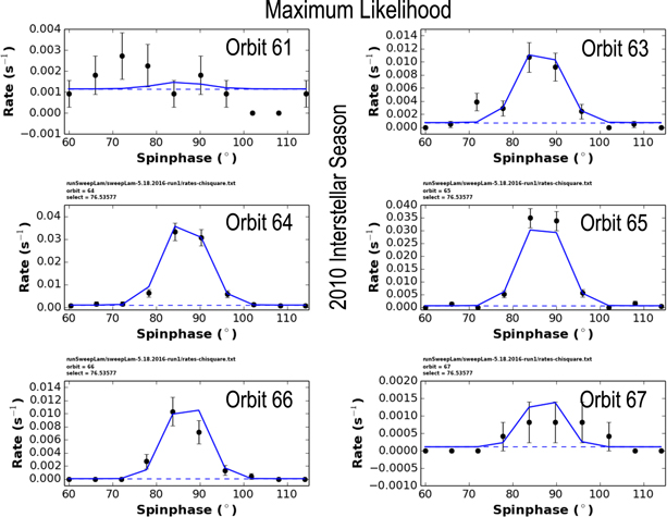
Figure 9. Comparison between modeled (blue curves) and observed rates during the 2010 interstellar season for the best-fit parameters using maximum likelihood (Table 4). Dashed lines show the background rates found in each orbit.
Download figure:
Standard image High-resolution imageBased on the results of the maximum likelihood analysis, we derive the parameter tube for the interstellar temperature (Figure 10, top) and speed (Figure 10, bottom) as a function of interstellar longitude. The derived temperature parameter tube for interstellar O and interstellar He are almost identical. At the flow longitude of 76°, the O temperature is ∼1000 K greater than the He temperature. This constitutes less than a ∼11% difference.

Figure 10. Comparison of derived parameter tubes using maximum likelihood fits for interstellar temperature (top) and interstellar speed (bottom) as functions of flow longitude for O (in blue) and He (in red; Schwadron et al. 2015). Thick solid curves show parameter tubes for the combined 2009–2010 data, and thin solid tubes show corresponding uncertainty regions. Dashed and dotted curves show the parameter tubes derived for the 2009 and 2010 seasons separately. The close correspondence between 2009 and 2010 parameter tubes indicate the stability of the fits for the peak latitude.
Download figure:
Standard image High-resolution imageFigure 10 reveals that the derived interstellar speeds are almost statistically distinct at the 1σ level. At the flow longitude of 76°, the interstellar O speed would need to be ∼0.95 km s−1 higher than the interstellar He speed.
It is noteworthy that while the parameter tubes are close to one another in the 2009 and 2010 seasons, the inferred inflow longitudes are quite different. Using only 2009 data, we derive , and using only 2010 data, we derive . The large uncertainties and the large variation from season to season are indications of the significant degeneracy in interstellar parameters along the parameter tube.
The final parameters derived from maximum likelihood fits are the scaling constants Ak for 2009 and 2010. For the 2009 period (k = 1), we find A1 = (1.1 ± 0.1) × 10−5 cm−3 and for the 2010 period (k = 2), cm−3. We relate these scaling constants to an interstellar density in Section 6.
6. THE INTERSTELLAR DENSITY
Table 5 shows results for the interstellar O density using a χ2 and a maximum likelihood analysis. Since the scaling factor derived from fits represents an interstellar O density (near the termination shock) times the survival probability, we must have an estimate of the O ionization rate, taken from Bzowski et al. (2013a), in order to estimate the density.
Table 5. Results for the Interstellar O Density
| Parameter | 2009 | 2010 | 2009–10 |
|---|---|---|---|
| a (10−7 s−1) | 5.34 ± 0.53 | 5.05 ± 0.51 | ⋯ |
| (χ2) (10−5 cm−3) | |||
| (Max. Likelihood) (10−5 cm−3) |


Note.
aIonization rates from Bzowski et al. (2013a).Download table as: ASCIITypeset image
The IBEX results can be directly compared to the abundances determined from both pickup ions and anomalous cosmic rays because they are sampling the same population of interstellar atoms (e.g., those where the filtration has already occurred). The interstellar density of He determined from pickup ions is estimated at 1.5 × 10⁻² cm−3 (Gloeckler 1996). The O/He abundance from pickup ions is estimated as (Geiss et al. 1994). Taken together, these observations indicate a neutral density in the outer heliosphere (near the termination shock) for O of cm−3. From anomalous cosmic-ray data, Cummings et al. (2002) derives an O density in the outer heliosphere (near the termination shock) of cm−3. Both results are consistent, within uncertainties to the interstellar O density cm−3 found here.
![$[{\rm{O}}/\mathrm{He}]={3.5}_{-1.4}^{+1.8}\times {10}^{-3}$](https://content.cld.iop.org/journals/0004-637X/828/2/81/revision1/apjaa3280ieqn155.gif)


7. DISCUSSION
The flow longitude derived for interstellar O of 760 ± 34 from χ2 analysis and 765 ± 62 from a maximum likelihood fit is compatible with the derived flow longitude of interstellar He, 75.6 ± 1.4 (Schwadron et al. 2015). Drews et al. (2012) used STEREO data to determine the longitude of the O flow vector using the upwind crescent formed by O pickup ions. They found a flow longitude of 789 ± 31. This longitude is consistent with the IBEX value to within uncertainties. Note also that transport effects acting on pickup ions tend to increase the longitude observed for pickup ions relative to their progenitor neutral atoms. This effect would reduce the inferred flow longitude based on the pickup ion observations (Chalov & Fahr 1999), which likely brings the IBEX and STEREO observations into even closer agreement. Sokół et al. (2016) show that the latitudinal anisotropy of the rate of charge-exchange between ISN O and solar wind protons is due to the latitudinal structure of the solar wind. This anisotropy in latitude likely biases the longitude of the ISN O inflow derived from PUI observations (Drews et al. 2012) by an amount comparable to the difference between the PUI O inflow longitude and the most recent IBEX ISN He inflow longitude (McComas et al. 2015b).
We compare the results derived here for interstellar O (green data point) with interstellar He and other species in Figure 11. This figure is a variant of that developed by Schwadron et al. (2015c) showing the triangulation of the direction of the local interstellar magnetic field. Blue and cyan curves show the great circle projections of connecting interstellar He (blue for IBEX, and cyan for Ulysses; Witte 2004; Schwadron et al. 2015) with the interstellar H measured by SOHO/SWAN (Lallement et al. 2005, 2010). The dashed blue curves show the uncertainty limits of this projection. These curves define what is often referred to as the "neutral deflection plane" of the "B–V plane."

Figure 11. Direction of interstellar neutral O measurements (green) is shown in the context of other interstellar determinations. Panel (a) includes all measurements, and panel (b) is a blow-up focusing on interstellar O, He, and H measurements. Interstellar neutral He atoms, due to their high first ionization potential, predominantly survive the journey from the interstellar medium into 1 au. Therefore, interstellar He represents a particularly good sample of the interstellar flow. In contrast, charge-exchange between protons in the outer heliosheath and inflowing interstellar neutral H causes the slowing, heating, and deflection of the neutral H. SOHO/SWAN detects the Lyα resonant backscatter from the inflowing H, providing the average flow direction of interstellar H inside the heliosphere (Lallement et al. 2005, 2010). Deflection of H relative to He measured by IBEX or Ulysses provides a plane (the so-called B–V plane) that is believed to contain the direction of the interstellar magnetic field since it breaks the flow symmetry of the global heliosphere (Lallement et al. 2005; Schwadron et al. 2015c). The blue curve shows the B–V plane containing the flow deflection of interstellar H relative to He based on measurements from SOHO/SWAN and IBEX. Dashed blue curves show the uncertainty limits of the B–V plane. The gray curve is the B–V provided by fitting secondary He in addition to H and primary He (Kubiak et al. 2016). Also shown is the B–V plane (purple curve) based on measurements from SOHO/SWAN and Ulysses. The centers of the IBEX ribbon (Funsten et al. 2013, black points) line up well with the projected B–V plane. The direction of the interstellar magnetic field measured by Voyager 1 (Schwadron et al. 2015c) also lines up well with the B–V plane and the ribbon center when projected out in time based on the observed temporal gradient in the field direction.
Download figure:
Standard image High-resolution imageThe gray data point shows the direction of the ISN He "warm breeze" (Kubiak et al. 2014, 2016), the secondary neutral component created by charge-exchange between ISN He and the plasma in the heliosheath. The warm breeze is both substantially hotter and slower than the primary neutral He from the LISM. Kubiak et al. (2016) found a flow direction of the warm breeze, which is coplanar (the best-fit B–V plane including secondary He, primary He, and H is shown in gray in Figure 11) with the flow directions of ISN H and ISN He, and the direction to the center of IBEX Ribbon within uncertainties (Funsten et al. 2009b, 2013; Fuselier et al. 2009a; McComas et al. 2009a; Schwadron et al. 2009). This co-planarity lends support to the hypothesis that the warm breeze is the secondary population of ISN He and that the center of the Ribbon coincides with the direction of the local interstellar magnetic field.
One of the interesting features of the interstellar O direction found here is that the latitude is below that of both the primary interstellar He component and the secondary component (the warm breeze). Figure 12 provides a schematic that helps explain the latitude shifts in the secondary He warm breeze, and interstellar O, which is more strongly filtered by the heliosheath than primary neutral He. The draping of the local interstellar magnetic field causes compression and shifts the pressure maximum in observed ENAs (in the globally distributed flux, which excludes the ribbon) south of the upwind direction (Schwadron et al. 2014). This added compression south of the upwind direction thins the outer heliosheath, providing preferred access to primary neutrals from the interstellar medium due to weakened filtration. In contrast, secondaries created within the outer heliosheath should have a slight bias for being created at latitudes above the upwind direction. These effects would tend to shift the secondary upwind direction above (north of) the primary He upwind direction in latitude, but shift the interstellar O upwind direction below (south of) the primary He upwind direction in latitude, as observed (Figure 11).

Figure 12. (Top) Schematic of global heliosphere showing compression of heliospheric boundaries southward of the upwind direction. This compression creates conditions that weaken filtration of incident neutral atoms southward of the upwind direction. In contrast, the thickened outer heliosheath to the north of the upwind direction provides for the creation of additional secondaries. (Bottom) Figure adapted from Schwadron et al. (2014) showing the asymmetry in the energetic neutral atom pressure times line of sight. The line of sight integrated pressure maximum is shifted south of the upwind direction, presumably due to compression by the draped local interstellar magnetic field.
Download figure:
Standard image High-resolution image8. SUMMARY AND CONCLUSIONS
We have presented the first detailed analysis of IBEX ISN O observations, providing entirely new information on the flow properties of this important interstellar population. The key areas of development are summarized as follows:
- 1.Deriving the local interstellar properties of oxygen is important for understanding nucleosynthesis. Because interstellar O undergoes significant amounts of charge-exchange, its ionization rate is important for backing out abundances from measurements made inside the heliosphere. One of the key parameters derived from our fitting analysis is the survival probability times the ISN O density, cm−3 based on χ2 fitting and (1.1 ± 0.1) × 10−5 cm−3 based on maximum likelihood fitting. For ionization rates (referenced to 1 au) from Bzowski et al. (2013a; see Table 5), our observations require a density of cm3 for χ2 fitting and cm−3 based on maximum likelihood fitting. These estimates are remarkably close to previous estimates (e.g., Geiss et al. 1994; Gloeckler 1996; Cummings et al. 2002).
- 2.We have derived the interstellar parameter tube relationships for primary interstellar O. The relationship between interstellar temperature and longitude overlaps with and is consistent with the corresponding parameter tube for primary interstellar He. In contrast, the parameter tube for interstellar O speed is systematically higher than for primary interstellar He. This difference is likely the result of enhanced filtration of O atoms through the heliosheath. The interaction of interstellar of O in the heliosheath is somewhat analogous to the interaction of primary interstellar H since both species have relatively large charge-exchange ionization rates. Charge-exchange interactions for both primary neutral H and O in the outer heliosheath represent a loss process, which has been quantified (e.g., Izmodenov et al. 2004). Such loss processes act preferentially on slower atoms due to the energy dependence of the charge-exchange cross section (Izmodenov et al. 2001; Katushkina & Izmodenov 2010). As a result, simulations show that filtration causes a ∼1–2 km s1 average increase of the primary flow speed and a few hundred kelvin reduction in the effective temperature of the primary distribution function (Izmodenov et al. 2001). Note that we observe a ∼1 km s−1 faster primary population of O compared to He. The signature (faster O flow) is characteristic of the filtration process.
- 3.The upwind flow latitude of interstellar O is +44 ± 03 for χ2 fitting and +447 ± 056 for maximum likelihood fitting, which is southward of the interstellar upwind flow latitude of interstellar He, +512 ± 027. The upwind flow latitude of secondary He (the warm breeze) is found by Kubiak et al. (2016) to be +1195 ± 067. The deviation between the warm breeze and primary He flow suggests that the asymmetric latitude structure of the heliosheath leads to the preferential addition of secondary neutral atoms north of the upwind direction, and therefore causes the secondary upwind direction to be northward of the upwind primary direction. This also suggests that the southward deflection of the upwind flow latitude of interstellar O may be the result of filtration in which the compressed heliosheath southward of the primary upwind direction provides preferential access to the heliosphere for primary oxygen atoms (see Figure 12).
- 4.The temperature of primary interstellar O is found to be remarkably consistent with that of He. The optimal fit temperature of oxygen at a reference flow longitude of 76° is ∼600 K less (for χ2 fitting) and ∼1000 K greater (for maximum likelihood fitting) than the corresponding helium temperature at this longitude. This difference in temperatures is extremely small, within ∼10%. We measure the states of neutral atoms, which interact with ions in the interstellar medium through collisions and charge-exchange. (Note that neutral O thermodynamics should be closely coupled to neutral H thermodynamics, which in turn is coupled to protons through charge-exchange and through ion-neutral dipole coupling; Spangler et al. 2011.) Collisions will tend to create Maxwell–Boltzmann-shaped velocity distributions with roughly equal temperatures for different species. However, mass-dependent heating, which is often found in even moderately turbulent plasmas such as the solar wind near 1 au (e.g., Hefti et al. 1998), would render ion velocity distributions closer to a state with equal thermal (or random kinetic) speeds. This would cause heavy ion distributions such as O to have much higher temperature than light ion distributions. The fact that ISN atom distributions show roughly equal temperatures for He and O indicates that collisions maintain equilibrium temperatures of ions and neutrals. High levels of turbulence in the interstellar medium would cause differentiation in the temperatures of O and He. Therefore, turbulence must be relatively weak in the local interstellar cloud near the solar system.
We have provided the first detailed analysis of ISN oxygen properties using IBEX data. We have shown that the interstellar oxygen parameters are similar to those of the He primary component. In particular, the best-fit O and He temperatures are within ∼10% at a reference flow longitude of 76°, which provides a strong indication that the local interstellar plasma near the Sun is relatively unaffected by turbulent heating. We also observe key differences between primary oxygen and helium. The parameter tube (relation between speed and longitude) for oxygen has interstellar speeds larger than the corresponding speeds in the parameter tube for He, and the flow latitude for oxygen is closer to the ecliptic plane. Both of these differences may be the result of enhanced filtration of interstellar oxygen due to its higher charge-exchange ionization rate compared to helium. Further, we derive the interstellar O neutral density that, within uncertainties, is consistent with previous estimates. Thus, we use IBEX data for the first time to probe the interstellar properties of oxygen.
We are grateful to the many individuals who have made the IBEX project possible. This work is supported by the Interstellar Boundary Explorer mission as a part of NASA's Explorer Program and partially by NASA SR&T Grant NNG06GD55G, the Swiss National Science Foundation, PRODEX, and the Polish National Science Center grant 2015-18-M-ST9-00036. Support for NAS also provided by a NSF grant (Sun-2-Ice, grant AGS1135432). Finally, we thank the International Space Science Institute for supporting discussions of the maximum likelihood approach used here as part of the research team: Radiation Interactions at Planetary Bodies (http://www.issibern.ch/teams/interactplanetbody/).
APPENDIX A: IBEX-LO GEOMETRIC FACTOR FOR ISN O
The geometric factor of IBEX-Lo for heavy neutral atoms, such as O, is controlled by the combination of surface conversion and sputtering to negative ions. As a consequence, the peak of the effective response in energy EPeak is always noticeably below the energy of the incoming neutral atom EIn, with this energy reduction factor R = EPeak/EIn decreasing with the energy EIn of the neutral atoms. In addition, the sensor detects these neutral atoms as negative ions over a broad range in energy around the peak energy EPeak due to the large acceptance range ΔE/E = 0.7 of the ESA and the broad range over which sputtered ions are generated. Therefore, the geometric factor that needs to be applied to a given combination of incoming energy EIn and IBEX-Lo energy step n (E-Step n = 1 8) depends on the absolute efficiency as a function of EIn, the reduction factor R, and where along the energy response function, relative to EPeak, the energy of energy step n En lies.
To obtain such a geometric factor calibration, the energy response curve of the sensor is needed, how its peak energy varies with the incoming energy of the neutral atoms, and the absolute geometric factor as a function neutral atom energy. It turns out that based on various calibration runs with an O beam during final calibration before flight, a combined normalized energy response curve could be constructed, normalized to the peak efficiency and the peak energy for each beam energy. The best-fit energy response curve to the combined calibration data set yields


where δ = 0.59. This functional dependence remains constant over the energy range of IBEX-Lo. The reduction factor R(EIn) as a function of beam energy EIn has been derived from a series of energy response measurements as:

where R0 = 1.04 and R1 = 0.134. ISN O arrives during the early spring ISN flow observation season in the IBEX frame at 1 au with a bulk energy of ≈540 eV. If secondary O is included in the analysis, the range of O energies in the IBEX frame falls between 540 and 435 eV, the energy of O atoms arriving on bounding parabolic trajectories starting with 0 eV outside the heliosphere. This energy range is between IBEX-Lo energy E-steps 5 and 6, which are the only steps of interest here. The signals in E-step 4 and the lower steps are completely controlled by ISN He (Möbius et al. 2009, 2012), and the O signal is too weak in E-step 7 to be of much use.
To determine the absolute geometric factor for E-steps 5 and 6, we used calibration results obtained with a neutral O beam EIn = 279 and 601 eV, the nominal incoming energies for these two steps, with the IBEX-Lo response taken at the same energy step and all the way down to energy step 1. Using Equations (10) and (11) the energy response curve was then fitted to the set of calibration results for E-step 5 and 6, adopting the same ±35% uncertainty for the absolute efficiency of each calibration point. To get the values for the two bounding energies of ISN O, the geometric factors at EPeak for the two E-steps were linearly interpolated. Table 6 shows the resulting geometric factors for the ISN bulk flow energy (540 eV) and for ISN O on a parabolic trajectory (435 eV). Listed are the geometric factors at EPeak for these input energies at the top, followed by the geometric factors for observations in E-step 5 and 6.
Table 6. Geometric Factors for ISN O
| Parameter | ISN O | ISN O (ISN Traj) |
|---|---|---|
| (eV) | 540 | 435 |
| GF at EPeak (cm2 sr) | 9.6 ± 3.4 10−5 | 8.7 ± 3.0 10−5 |
| GF at E-Step 5 (cm2 sr) | 8.8 ± 3.1 10−5 | 8.6 ± 3.0 10−5 |
| GF at E-Step 6 (cm2 sr) | 5.6 ± 2.0 10−5 | 2.2 ± 0.8 10−5 |

Download table as: ASCIITypeset image
APPENDIX B: STATISTICAL AND PROPAGATION UNCERTAINTIES
We examine the fitting of the M-parameter statistical model to the given data set , by minimizing the χ2

Here yi is the number of counts. The global minimum of the χ2 give the parameter optimal values, , by solving the system of equations,

After solving the system of these M equations, we derive the parameter optimal values as functions of data points,

For simplicity, we have indicated only dependence on data (y) values.
The statistical error (also called the curvature error) of the optimal value is given by


for m = 1, 2, ..., M and is the Hessian matrix of the χ2 at the global minimum. The quantity is the mth diagonal element of the Hessian inverse matrix (Livadiotis 2007). The estimated χ2 value is


and is the reduced χ2 value (the degrees of freedom are N − M).

We generalize the statistical error for use in maximum likelihood fitting techniques. Consider an arbitrary distribution function Pi = f(yi, Vi). The joint probability distribution over the set is , or, by taking its logarithm,


The likelihood is defined by this joint probability, but it is more often used with the inverse function and its logarithm,

where c is an arbitrary constant (typically taken to be c = 2). The inverse likelihood ℓ is a function of the fitting parameters, ℓ(p1, p2, ..., pM) and needs to be minimized, corresponding to the minimization of the χ2 in the case of normally distributed data. The Taylor expansion of around its minimum value, , gives


Since this expansion is performed about an extremum, the second term in the expansion drops out, resulting in the following:

where the curvature matrix is half the Hessian,


The statistical independent uncertainty in this case is given by

There is another type of error that characterizes the uncertainty in parameter optimal values and involves the propagation of the measurement uncertainties . This propagation uncertainty is given by


for m = 1, 2, ..., M.
The two types of uncertainty are fundamentally distinct: the curvature error is not strongly dependent on the measurement uncertainties . In contrast, the propagation error is based directly on a weighted sum of the squares of measurement uncertainties. For example, if all measurement uncertainties are equal to σ, the propagation error becomes directly proportional to the common measurement uncertainty, . Because both uncertainties are distinct, they must both be included in the final uncertainty estimation. A rough approximation for the total uncertainty (see, for example, Schwadron et al. 2013) is given by


APPENDIX C: MINIMIZATION OF χ2 FOR DERIVATION OF BACKGROUND RATES AND A MODEL SCALING FACTOR
In this section we discuss how minimization of χ2 can be used to derive orbit-by-orbit background rates and the scaling factor that multiplies the spin-phase distribution. Observed rate distributions as a function of spin-phase are represented by where the first index i corresponds to the orbit number, and the second index j refers to the spin-phase. These rate distributions are accumulated over the good times for a specific orbit. The model has dependencies on the instantaneous velocity and pointing of the spacecraft, and the instantaneous pointing of the IBEX-Lo instrument. As a result, the model simulations must also accumulate rates over the good time periods, and over the angles swept out over a given spin-phase bin. Therefore, the rate distribution modeled simulates the actual instrument response precisely.


The modeled rate distributions scale linearly with a factor that depends on the density times the survival probability, × Sp. Therefore, it is convenient to define an overall scaling factor for the modeled rates. Here nref and are a reference density and a reference survival probability. The scaling factor Ak should be roughly fixed in each interstellar season, but could vary from season to season. The scaling factor therefore depends on the year of observation, indexed by k. The model distribution is expressed:


Only specific orbits i exist in a given year and we treat the index (k) as an implicit value. The quantity represents simply the unnormalized modeled rate,


This unnormalized model distribution incorporates the effects of survival probability, integration through the instrument response, and all the factors involved in translating fluxes from the outer heliosphere to IBEX at 1 au.
There is also a background rate, Bi, that typically varies from orbit to orbit. We treat this background rate as a constant rate in the spin-phase distribution in a given orbit, which is added to the rate derived from interstellar atoms. Therefore the modeled spin-phase distribution in a given orbit is defined by

and the corresponding χ2 is given by

where σij is the uncertainty in the observed rate.
We solve for the background rate and scaling factor by minimizing the χ2 explicitly. We solve , which yields


where the effective observed rate is


and the effective model rate is


In order to solve for the scaling factor Ak and its uncertainty , we express the χ2 as a quadratic function of Ak with a minimum at :


By setting Equation (32) equal to Equation (28) we may solve for the coefficients C0, , and C2:


This formulation is similar to that used by Schwadron et al. (2013), where it is shown that the statistical uncertainty of the χ2 minimum from a quadratic form is

where ν is the number of degrees of freedom.
The propagation uncertainty follows from the traditional treatment of error propagation

We note further that C0 is the minimum of the χ2 and that the reduced χ2 (denoted ) at the global minimum is given by,


Therefore, the statistical uncertainty is directly related to the propagation uncertainty,

which results in a total uncertainty given by

This result can be readily interpreted. The minimum reduced χ2 amplifies the propagation uncertainty. A poor fit results in a large value of and thereby increases the total uncertainty. The propagation uncertainty represents the minimum possible uncertainty in the presence of a particularly good fit. A statistically likely fit with results in a total uncertainty that is larger than the propagation uncertainty.


In this case, there are two sets of variables to determine from explicit χ2 minimization: the background rate Bi determined on an orbit-by-orbit basis; and the scaling factor Ak determined for each interstellar season in a given year. The task is to find a χ2 minimum as a function of both the background rates and the scaling factor. We find this two-dimensional (2D) χ2 minimum through successive iterations: we find the background rates, then use those background rates in the solution for the amplitude, and then solve again for the background rates, and so forth. This scheme converges quite quickly (typically within three steps) to the 2D χ2 minimum.
APPENDIX D: MAXIMUM LIKELIHOOD FOR DERIVING BACKGROUND RATES AND A MODEL SCALING FACTOR
We use maximum likelihood to calculate background rates and a model scaling factor in a manner similar to the derivation in Appendix C. Specifically, the model is specified as

where Ak is the scaling factor and Bi is the background rate. In this case, we must specify the expected counts ,


where is the exposure time. Using this expectation value, the probability of observing counts is


The inverse likelihood is expressed as
where the summation extends over only those orbits associated with a given season k.
The minimization of ℓk with respect to the background rate Bi, , leads to the relation


The constant Bi is varied using a search algorithm to find the optimal value. We minimize the inverse likelihood with respect to the amplitude, Ak, , leading to


where the summation extends over only those orbits associated with a given season k. A search algorithm is used to find the optimal amplitude.
APPENDIX E: STATISTICAL AND PROPAGATION UNCERTAINTIES IN NONLINEAR FORWARD MODELS USING χ2 MINIMIZATION
As discussed in Appendix B, there are two forms of uncertainty included in our calculations: the statistical and propagation uncertainty. In a previous section (Appendix B), because we are able to solve for the model scaling factor analytically, it is relatively straightforward to directly solve for both the statistical and propagation uncertainties. The difficulty arises however in nonlinear forward models where there is no closed form analytic solution to determine best χ2 fits for model parameters. In this case, we must find alternative solutions to derive the best-fit parameters and their uncertainties. This appendix develops a relatively straightforward and robust technique for deriving these uncertainties.
The χ2 analysis used in this paper is five dimensional. It is useful here to consider a nonlinear forward model with one parameter, p. The is minimized to find a best-fit at p = . We consider a series of N measurements with uncertainties and corresponding simulated values . The χ2 is defined:


Because the χ2 has a minimum, its dependence on p can be approximated as a quadratic:

The statistical uncertainty is then

where ν is the number of degrees of freedom: and the number of model parameters is M = 1.

The propagation uncertainty is calculated as follows:

The difficulty in this case is that there is no closed-form solution for , which makes it cumbersome to solve Equation (50).

One option for solution is to approach the problem numerically. We go through each measurement and vary the measured value through Oi ± σi. As we perform this variation, we solve for the χ2 and find how variation in Oi causes variation in the χ2 minimum. This allows us to solve for . We then move to the next data point , vary the data point , find the change in , and solve for .


There are two problems with this solution. First, if the number of measurements N is large, which is typical, then the calculation becomes extremely costly to compute. The second problem is that finding the χ2 minimum often involves interpolation. Therefore, finding the effects of extremely small changes to χ2 and the resulting small changes in is likely to be difficult to compute accurately.

There is another way to approximate the changes to , that is far more straightforward to implement and interpret. We consider the solution for as a weighted average of individual terms pi, which represent the model parameter based on a given observation Oi. The average for is weighted by the inverse of parameter variances (to be detailed as follows):


In formulating this solution, we use the model to estimate how individual terms in the summation, pi, change based on variations in the observed data Oi. Specifically, we use partial derivative to estimate how a change in a given observation ΔOi leads to a change in the model parameter Δpi:


In order to turn this estimate of Δpi into an estimate of pi itself we must simply include a constant , such that


Since we are concerned only with small changes in pi resulting from changes in Oi, it is important only that the constant is fixed while Oi is varied.

Similar reasoning is applied to find the variance of the parameter based on the variance observed using to convert observed variances into parameter variances:


By substituting Equations (53) and (54) into (51), we recover the following solution for

Equation (55) is now substituted into (50) to find the variance in :


This solution for the propagation uncertainty may be used directly. There is a further simplification when we consider the original form of the χ2 minimum. We treat the model solutions as a second-order expansion about the optimal solution:
Substitution of this second-order expansion into the χ2, Equation (47), results in the following when we retain terms up to the second order in :

Because the solution exists at the minimum of the χ2, the term that is the first order in must vanish:


Notice also that we may now relate the constants in Equation (48) to the terms in the expansion:


where we have neglected the second-order derivative from C2. This approximation, which is commonly used, simplifies the analysis and, in practice, does not substantially change the amplitude of the second order term. This association, when applied to Equation (56) implies that


As in Appendix B, this then implies that

where is the minimum value of the reduced χ2. The total uncertainty is

As was found previously in Appendix B, the statistical uncertainty is an amplification of the propagation uncertainty where the term serves as an amplification factor.

The propagation uncertainty is related to the covariance. For example, in Press et al. (1992), the curvature matrix (one half times the Hessian matrix) is found to be

where pk is a given parameter in a multidimensional fit. The covariance matrix is the inverse of the matrix [α]:


and the diagonal elements of the covariance matrix constitute the variances of the parameters involved in the fit, which we show are in fact the propagation uncertainties,

When applied to a single-dimensional fit, we find that the curvature matrix reduces to the following constant

which is identically equal to C2. And the inverse of α is identically equal to the variance of the propagation uncertainty, , as found previously, Equation (62). Substitution of Equation (62) into (63) therefore yields


where H is the Hessian. Equation (69) is nothing less than a 1D form of Equation (15). The derivation comes full-circle, revealing the consistency of the derived terms for the statistical and propagation uncertainties.
The discussion in Section 3 applies to the derivation of the parameter tube for interstellar parameters, which exists in 4D parameter space. This constitutes a multi-parameter fit using χ2 minimization. The parameter tube is itself an expression of the underlying relationship between interstellar parameters. And because the interstellar speed and interstellar temperature are varied along the parameter tube when finding the χ2 minimum in the interstellar longitude, the covariance between parameters is handled explicitly. As a result, it is appropriate to treat uncertainties using the 1D equations for the propagation and statistical uncertainties: Equations (62) and (63). It must be appreciated however that the uncertainty in interstellar speed and interstellar temperature define the width of the parameter tube in their respective dimensions. The uncertainty in the interstellar longitude applies along the parameter tube and provides the most significant covariant uncertainty in determining the interstellar speed and temperature.
It is also apparent that utilization of the covariance alone determines only the propagation uncertainty. The statistical uncertainty is an additional and independent contribution that inflates the total uncertainty.
APPENDIX F: STATISTICAL AND PROPAGATION UNCERTAINTIES IN NONLINEAR FORWARD MODELS USING MAXIMUM LIKELIHOOD
The main difference between χ2 minimization and maximum likelihood is the approach to metric used to relate observations and model predictions. We consider bin i of the number of counts observed oi or modeled mi. Note that there is an important distinction between the counts within bins used here and the rates used in Appendices B and C. The exposure time Δti is used to relate rates to observed or modeled counts:


We treat the observed events within each bin oi as a random Poisson distribution with expectation value mi,

The χ2 is related to the joint probability associated with a Gaussian distribution, PGi, by . The corresponding quantity in the case of Poisson distribution is

The maximum likelihood is found by minimizing ℓ with respect to a parameter p:

The counterpart for solving for an extremum in the minimization of χ2 is

The variance can be derived precisely based on the curvature of :


It should be noted in this relation that the inverse variance is related to the curvature with respect to variation in the model, as opposed to the curvature with respect to variation in observation. The reason for basing the uncertainty on model variation is that the model is a continuous variable, and, as a result, the curvature can be defined accurately even when the observed counts are low. Applying the relation in Equation (76) to the Poisson distribution, we find the following definition for the inverse variance:

We apply the same approach as that in Appendix C to derive the propagation uncertainty,

where we have used Equation (77) to relate the variance to expected counts in a bin. We expand the ℓ to the second order in :

where . We neglect terms involving second derivatives of mi and the first-order term vanishes since we are at an extremum. With these simplifications, we find the following quadratic form for ℓ:


Therefore, we find that the propagation and statistical uncertainties are


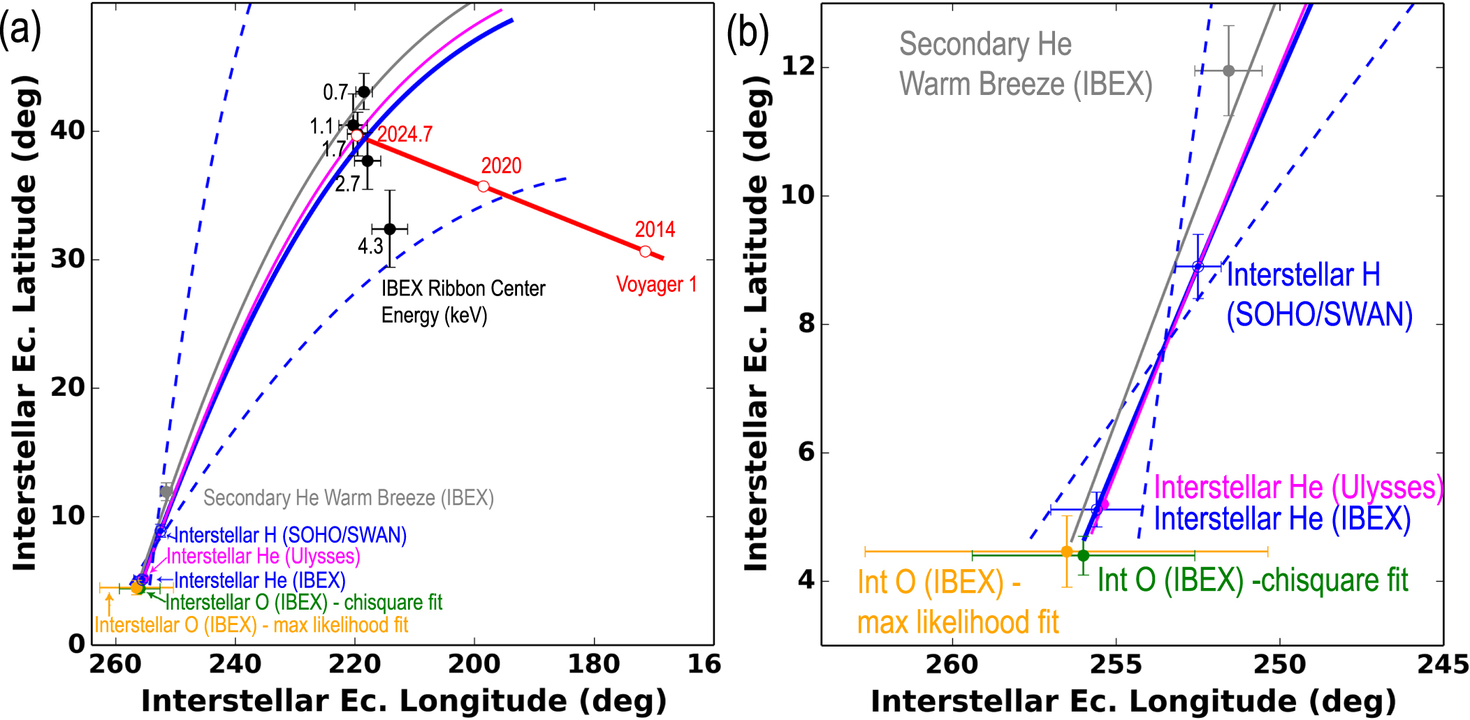