


ABSTRACT
The problem of a cold gas flowing past a stationary obstacle is considered. We study the bow shock that forms around the obstacle and show that at large distances from the obstacle the shock front forms a parabolic solid of revolution. The profiles of the hydrodynamic variables in the interior of the shock are obtained by solution of the hydrodynamic equations in parabolic coordinates. The results are verified with a hydrodynamic simulation. The drag force on the obstacle is also calculated. Finally, we use these results to model the bow shock around an isolated neutron star.
Export citation and abstract BibTeX RIS
1. INTRODUCTION
Bow shocks occur when a supersonic flow encounters an obstacle. Prominent examples from astrophysics include planetary bow shocks (Treumann & Jaroschek 2008), inundation of a dense molecular cloud by a supernova shock wave (McKee & Cowie 1975), and bow shocks around stars that move at a supersonic velocity relative to the interstellar medium (ISM) (Noriega-Crespo et al. 1997).
The last decades have yielded a plethora of analytic and numerical works on hydrodynamic bow shocks (as opposed to MHD bow shocks). Farris & Russell (1994) studied the different factors affecting the distance between the obstacle and the nose of the shock front. Wilkin (1996) considered a radiative (fast cooling) bow shock that forms when an object moves relative to a uniform medium, while also emitting an isotropic wind. Cantó & Raga (1998) considered a radiative bow shock that forms when a solid sphere moves relative to a uniform medium. Verigin et al. (2003) developed a semi-analytic theory for the shape of an adiabatic bow shock around a parabolic obstacle. Schulreich & Breitschwerdt (2011) developed a topological theory in order to solve the inverse problem: determining the shape of the obstacle from the shape of the shock. Brighenti & D'Ercole (1995) performed 2D simulations for the bow shock formed around a wind-emitting red supergiant (RSG) moving relative to the ISM. Mohamed et al. (2012) performed similar simulation in 3D for Betelgeuse. Miceli et al. (2006) performed simulations for the bow shock that forms when a supernova shock wave sweeps a dense cloud. Comeron & Kaper (1998) performed simulations of an OB star moving through the ISM. van Marle et al. (2011) also simulated the bow shock around a moving RSG, but included the effect of dust in the calculation.
Despite the work mentioned above, there remains an unexplored niche in parameter space. That niche is an adiabatic shock of infinite Mach number, and it is the focus of this work. We assume that the incoming matter is cold, so for any finite velocity its Mach number would be infinite. The asymptotic shape far from the obstacle is qualitatively different from the case of a finite Mach number M. In the latter, far away from the obstacle, the size of the obstacle becomes irrelevant, and the shock front coincides with the Mach cone, i.e., a cone with an opening angle  (Landau & Lifshitz 1987, p. 467). When the Mach number tends to infinity, the opening angle of the Mach cone tends to zero. Hence the bow shock in that case cannot be straight, and the curvature must still be significant at large distances from the obstacle. In this paper we show that the shape of the shock is a parabola. We develop the mathematical theory to describe the shape of the shock and the profile of the hydrodynamic variables within, and then verify our supposition using a numerical simulation.
In astrophysical bow shocks, the wind of the external medium brakes by means other than direct collision with the compact object (a star, planet etc.). The braking mechanism could be magnetic fields or winds emitted from the compact object. The effective size of the obstacle is determined by the condition that the inner and outer pressures balance. In the case of a magnetic obstacle the effective radius of the obstacle is where the magnetic pressure balances the ram pressure of the outside wind:

where μ is the magnetic dipole moment,  is the density of the external medium, and vo is the relative velocity between the obstacle and the external medium. In the case of a wind obstacle, the stand-off distance is given by the balance of ram pressures of the inner and outer winds:

where  is the mass loss rate from the inner wind and vi is its velocity (relative to the object emitting it). In the latter case the contact discontinuity between the inner and outer winds serves as an effective rigid obstacle, because energy and matter do not cross that surface. Moreover, at increasing distances from the object, the fraction of enclosed mass and energy from the inner wind disappears.
This paper is organized as follows. In Section 2 we describe the complete mathematical formulation. In Section 3 we present validation of our analytic results with a numerical simulation. In Section 4 we calculate the drag force of such a shock. In Section 5 we present a manifestation of this solution in an observation. Finally, in Section 6, we discuss the results.
2. MATHEMATICAL FORMULATION
In this section we develop the mathematical equation to describe the shape of the bow shock and the profiles of the hydrodynamic variables inside it. We begin with an intuitive explanation for the asymptotic shape of the shock, proceed by giving a complete description of the steady-state interior of the shock using parabolic coordinates, and end with a discussion of the growth of the bow shock.
2.1. Intuitive Explanation for the Shock's Shape
In this subsection we perform an order-of-magnitude calculation for the shape of the shock. For this purpose we neglect dimensionless constants of order unity, since we are interested only in the power-law index. Let us consider an obstacle of cross section R2 moving at a velocity v through a medium of density ρ. Since the velocity of the obstacle is much larger than the speed of sound, in each time interval Δt the obstacle deposits an amount of energy that scales as  into a small region. This energy creates an explosion. However, this explosion does not expand spherically, because it is sandwiched between two other explosions. Instead, it expands as a disc. The energy of the disc is
  , where r is its radius. From energy conservation we get
  . The position of the obstacle is given by
  , so
, so  . Hence the bow shock is parabolic.
2.2. Steady State
Spherical parabolic coordinates are given by


In these coordinates, the steady-state, azimuthally symmetric hydrodynamics equations take the following form. The conservation of mass is

The conservation of entropy is

where  is the specific entropy. Since there is no dissipation inside the shocked region, this equation is equivalent to energy conservation (Landau & Lifshitz 1987, p. 467). The conservation of momentum in each direction is
One of the momentum equations can be replaced by Bernoulli's equation

where c is the speed of sound. We found it most convenient to express the equations in terms of the density ρ, the sound speed c, and the two Mach numbers  .
.
We assume that the shock front coincides with a curve on which  is constant. The Rankine–Hugoniot boundary conditions at the shock front are (assuming strong shock/infinite Mach number)


where subscript a indicates a property of the ambient medium (upstream) and subscript s the value at the shock front (immediate downstream). Although an infinite Mach number was assumed, the correction for a finite Mach number scales as  (Landau & Lifshitz 1987, p. 467); we contend that the boundary conditionscan be applied to moderate values of Mach number without great loss of precision. At very high values of
  , the equations can be simplified. We assume that the variables vary with τ as the shocked values do, i.e., ρ is independent of τ,
  ,
,  is independent of τ, and
  . Using this approximation, τ can be eliminated from the hydrodynamic equations, and the problem reduces to a set of ordinary differential equation in σ. These equations can be integrated numerically, and we can obtain curves for ρ,
  , mσ, and
  . The asymptotic equations for the interior of the shock are

These equations can be integrated numerically from the shock front to the axis of symmetry to produce the complete profile. An example of such a profile, for  , can be seen in Figure 1, along with a comparison to a numerical simulation, which will be described in the next section.

Figure 1. Comparison of analytic profiles (blue) with the numerical simulation with a rigid obstacle (red) and a wind-emitting obstacle (green) at τ = 1.5. Top left is density, top right is the speed of sound, bottom left is σ Mach number, and bottom right is τ Mach number.
Download figure:
Standard image High-resolution image2.3. Growth of the Shocked Region
We describe the shock in a cylindrical coordinate system, where the  axis coincides with the axis of symmetry. In this section we consider a shocked region of finite extent, so there is some point where the r coordinate attains a maximum, and we denote that maximum by ϖ. The rate at which ambient matter accretes onto the shocked region is
  . Matter can only be compressed by a factor of a few (for reasonable values of γ), so the volume of the bow shock
  has to grow at the same rate:

Therefore, the farthest point from the obstacle on the axis of symmetry (on the lee side) moves at a constant velocity  . In the absence of other scales, that velocity has to be of the same order of magnitude as the incident velocity. For shocks with a finite Mach number,
  . Thus the age of a bow shock can be inferred from its size.
These results were verified with a numerical simulation (see next section). We examined the history of the mass enclosed within the bow shock. From the discussion above, it is clear that the mass scales with time as  . Figure 2 shows that indeed the mass is parabolic in time.
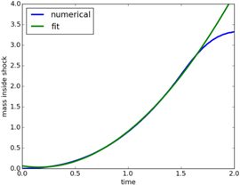
Figure 2. History of the mass enclosed inside the bow shock: comparison of the numerical result (blue) with a parabolic fit (green). The deviation at late times is due to truncation of the bow shock by the boundaries of the computational domain.
Download figure:
Standard image High-resolution image3. NUMERICAL SIMULATION
3.1. Solid Obstacle
To verify our results, we ran a simulation in the RICH code (Yalinewich et al. 2015). The simulations are in 2D cylindrical coordinates, assuming azimuthal symmetry. The boundaries of the computational domain are 180 > z > −20 and 25 > r > 0. We used a Cartesian grid with 100 cells in the r direction and 800 cells in the z direction. The velocity of the ambient medium is 1 in the positive z direction. The pressure was 10−9 and the density 1, which translates to a Mach number of more than 104. The obstacle is a circle of radius 1, located at the origin  . The adiabatic index used was γ = 5/3. We ran the simulation to time t = 1000 and compared the numerical results with our analytic predictions. A density map from the last time step of the simulation can be seen in Figure 4. First, we fit the shock front to an even parabola (Figure 3), i.e.,
  . As can be seen from the figure, the shock front does converge to a parabola when the distance from the obstacle is much larger than the radius. The coefficients obtained from the simulation are a = 0.474 and b = −9.67. The ratio between the curvature radius of the shock front and the radius of the obstacle in this simulation is
  . Next, we compared the numerical profiles inside the bow shock to the analytic prediction (Figure 1). In order to do that, we interpolated the variables on the curve τ = 1.5. The agreement between the two is reasonable. The deviations are due to two main reasons. The first is that since we are working in cylindrical coordinates, the relative error at each radius is equal to the ratio between the cell's width and the radius. The second is that the slope of the density is very steep next to the shock front, so a very fine resolution is required to resolve it. In the previous section it was shown analytically that very far from the obstacle the shock is parabolic, but the analytic theory did not constrain the shape of the shock front close to the obstacle (henceforth referred to as the "nose"). Since the only length scale in this problem is the size of the obstacle, the shape of the bow shock should scale as
  . The dimensionless function f can be obtained from the simulation. The ansatz chosen to represent f is a six-parameter Padé approximant in even powers of its argument:
Odd powers were excluded to avoid a cusp at the z axis. The choice of powers in the numerator and denominator reproduces the analytic asymptotic behavior  for
for  . The calibrated coefficients are given in Table 1. A comparison between the numerical and analytic results is presented in Figure 3, and the deviations between the two are shown to be quite small.

Figure 3. Comparison between the Padé fit (red), the parabolic fit (green), and the shock front obtained from the simulation.
Download figure:
Standard image High-resolution image
Figure 4. Density map from the last time step of the simulation with a rigid obstacle. The rigid obstacle is located at the origin. The upstream fluid flows from the bottom to the top.
Download figure:
Standard image High-resolution imageTable 1. Coefficients for the Ansatz (20), Calibrated from the Simulation
| c0 | −1.30 |
| c1 | −0.29 |
| c2 | −0.0548 |
| c3 | 0.0215 |
| c4 | 0.392 |
| c5 | 0.0404 |
Download table as: ASCIITypeset image
3.2. Wind Obstacle
The discussion so far has concentrated on a flow around a rigid obstacle. In astrophysics, however, it is extremely rare for a solid object to collide directly with diffuse matter. A more common scenario is that diffuse matter is halted at a distance much larger than the object itself, by magnetic field or by the wind emanating from the object. In this section we deal with the second case, which we refer to as wind-termination bow shock. In this case the effective radius of the obstacle (up to a dimensionless prefactor) is given by Equation (2). We claim that the formalism described above can also be used to describe bow shocks around wind obstacles. In order to put this idea to the test we ran another simulation, quite similar to the previous one, but instead of a solid obstacle we kept injecting matter into a small area around  . The velocity of the inner wind was ten times higher than the outer wind, and the mass loss rate was
  . At the other extreme, where the inner wind is much slower than the outer wind, the flow becomes unstable (Comeron & Kaper 1998; Decin et al. 2012). The shape of the forward shock front is given in Figure 5, and a density map from the last time step is given in Figure 6. The results of the simulation support our notion that the nature of the obstacle has very little effect on the shape of the bow shock around it.
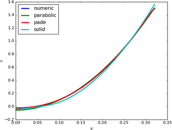
Figure 5. Shape of the shock front of a wind-termination bow shock (blue), parabolic fit (green), Padé approximation (red), and a scaled shock front for a bow shock around a solid obstacle (cyan). Whether the obstacle is solid or due to wind termination has very little effect on the shape of the shock.
Download figure:
Standard image High-resolution image
Figure 6. Density map of the simulation of a wind obstacle. The pointlike wind source is located at the origin. Upstream fluid flows from the bottom to the top.
Download figure:
Standard image High-resolution image4. DRAG FORCE
In this section we calculate the drag force on a rigid obstacle. In realistic cases, even dense clumps cannot withstand bow shocks indefinitely, and they eventually break up due to hydrodynamic instabilities. We can still justify this approximation by restricting it to the early times before the obstacle is disrupted.
From dimensional analysis one can infer an expression for the drag force,

where cd is a dimensionless drag coefficient. It is possible to obtain an analytic upper bound on cd. The highest pressure on the obstacle is at the stagnation point. This is the point on the surface of the obstacle that is closest to the nose of the bow shock. The component of the velocity normal to the obstacle vanishes on the surface of the obstacle, and due to symmetry considerations, the tangential velocity also vanishes at that point. Therefore, using Bernoulli's equation and the adiabatic relations, the pressure can be evaluated there (McKee & Cowie 1975):
So the upper limit on the drag force is  , and the upper limit on the drag coefficient is cd = 0.827 (for
  ). The drag coefficient can be evaluated numerically, using the pressure on the obstacle
  , where θ is the angle measured relative to the direction of the velocity of the ambient medium. If the pressure is known, then the drag force is given by

For the simulation described above, the numerical drag coefficient is cd = 0.426, which is approximately half of the upper limit discussed above. The assumption of a steady state can be justified only if the obstacle travels a distance much larger than its own radius before it experiences a significant change in velocity. This is equivalent to the condition that the density of the object be much larger than that of the ambient medium.
5. APPLICATION TO RX J1856.5-3754
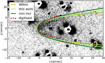
RX J1856.5-3754 is a neutron star that plows through the ISM at a speed of about 100 km s−1, and is adorned by a bow shock (van Kerkwijk & Kulkarni 2001). The bow shock sports Balmer lines, indicating that the ISM is not ionized, hence the temperature is below 104 K, so the Mach number is in excess of 10 (the magnetic field is bounded by equipartition (de Gouveia Dal Pino 2006) so the magnetic Mach number cannot be lower). Even if the Mach number is just 10, our solution for the shock should be valid within a distance of 100 times the size of the object. The distance between the neutron star and the nose of the bow shock is about 1'', and its tail extends to as far as 25''. Its distance is about 400 lt-yr and its inclination (angle between the line of sight and its velocity) is about 60°. The latter was inferred from measurements of proper motion and radial velocity. A comparison between our model and Hα observations (taken with the Very Large Telescope) can be seen in Figure 7. In order to perform the fit, we first manually digitized several points along the shock front.
van Kerkwijk & Kulkarni (2001) fit the observations to Wilkin's model (Wilkin 1996). The shock was shown to be adiabatic, whereas Wilkin's model assumes fast cooling. The figure below shows that our adiabatic model fits the observation. The analytic form used for our fit is the ansatz from (20). We note that in this fit we have only one free parameter, which is the size of the obstacle. We find that the best fit is obtained when this size is 0 9, which agrees with a previous estimate 1 ± 02 (van Kerkwijk & Kulkarni 2001). We note, however, that due to the uncertainties in the measurement, the fit to Wilkin's model is no worse than ours. In principle, it is also possible to use the fit between our model and the observations to estimate the inclination. Unfortunately, the data do not provide very stringent constraints, and only allow us to set a lower limit on the angle at 40°. From Figure 7 it is clear that inclination affects the wings of a bow shock more than it does the nose.
Figure 7. Comparison of our model (light green) with Wilkin's model (yellow) on top of the original observation (grayscale), taken from van Kerkwijk & Kulkarni (2001). Manually digitized points used for the fit are in red. The best fit with the inclination from van Kerkwijk & Kulkarni (2001) is in light green, and the fit with smallest inclination is in dark green. Our model seems to agree with observation. The fact that the nose is flatter than our model predicts is consistent with the simulation.
Download figure:
Standard image High-resolution image
6. DISCUSSION
We discussed the problem of a solid body traveling through a cold medium. We derived the steady-state, azimuthally symmetric hydrodynamics equations in cylindrical parabolic coordinates. We were able to use the approximation of very large τ to reduce these equations to a set of ordinary differential equations in σ. We numerically integrated these equations, and compared them to a full hydrodynamic simulation.
In the case of a large, but finite, Mach number, the bow shock would start out parabolic, but eventually straighten out and converge with the Mach cone. The transition will occur when the parabolic curve  intersects the Mach cone
  :
:


Therefore, the parabolic solution will only be valid in the region  .
.
Using these analytic results, we modeled the bow shock around RX J1856.5-3754. The fit is as good as that of Wilkin's model. However, Wilkin's model assumes fast cooling, whereas the presence of Balmer lines around that bow shock indicates slow cooling (Heng 2010).
Further work is required in order to apply this model to most astrophysical bow shocks. For example, planetary bow shocks require magnetohydrodynamics, supernova–cloud interactions involve a time-varying flow, and the complete description of the bow shock around Betelgeuse requires radiative cooling (Mohamed et al. 2012).
However, this model may apply to "knots" in supernova remnants (Fesen et al. 2006). These are bright, filamentary structures observed inside supernova remnants, but also sometimes outside the shock front. It is theorized that a fraction of the ejecta is in the form of small, dense gas clumps, and the filaments are the shocks they leave in their wake. Since they are much more compact than the rest of the ejecta, they are less affected by deceleration, and can therefore overtake the shock front. While inside the supernova remnant, their velocity is of the same order of magnitude as the bulk and thermal velocity of the ejecta. However, once they emerge from the shock front, the bow shock that will develop around them will be the epitome of the solution presented here.
Another utility of our solution is that it provides a lower bound on the width of an adiabatic bow shock. Bow shocks with lower Mach numbers are bound to be wider than the solutions described here.
This research was partially supported by ISF and iCore grants. We would like to thank Marten van Kerkwijk for allowing us to use the image from his paper. We thank Elad Steinberg, Nir Mandelker, and Prof. Chris McKee for enlightening discussions.