


ABSTRACT
Large-scale dynamo action is well understood when the magnetic Reynolds number (Rm) is small, but becomes problematic in the astrophysically relevant large Rm limit since the fluctuations may control the operation of the dynamo, obscuring the large-scale behavior. Recent works by Tobias & Cattaneo demonstrated numerically the existence of large-scale dynamo action in the form of dynamo waves driven by strongly helical turbulence and shear. Their calculations were carried out in the kinematic regime in which the back-reaction of the Lorentz force on the flow is neglected. Here, we have undertaken a systematic extension of their work to the fully nonlinear regime. Helical turbulence and large-scale shear are produced self-consistently by prescribing body forces that, in the kinematic regime, drive flows that resemble the original velocity used by Tobias & Cattaneo. We have found four different solution types in the nonlinear regime for various ratios of the fluctuating velocity to the shear and Reynolds numbers. Some of the solutions are in the form of propagating waves. Some solutions show large-scale helical magnetic structure. Both waves and structures are permanent only when the kinetic helicity is non-zero on average.
Export citation and abstract BibTeX RIS
1. INTRODUCTION
Dynamo action is often invoked to explain the origin of magnetic fields in astrophysics. In many cases the generated magnetic fields are organized on spatial and temporal scales much larger than that of the underlying turbulence. The process by which the magnetic field organizes itself on large scales is often termed the "large-scale dynamo problem." This is well understood when the magnetic Reynolds number (Rm) is small and first order smoothing applies, but becomes problematic as Rm increases; the magnetic fluctuations become dominant and obscure the large-scale behavior. This has led Cattaneo & Tobias (2014) to suggest that large-scale dynamo action is possible only if some mechanism exists to control the magnetic fluctuations. They proposed that this "suppression principle" could be mediated, for instance, by shear flows, diffusion, or nonlinearity. As their model was kinematic (i.e., neglected the back-reaction of the magnetic field on the flow) and at high Rm (i.e., very non-diffusive) they concluded that the suppression was associated with the shear. In their model the large-scale dynamo action manifested itself in the form of propagating dynamo waves of the type that had been predicted by Parker (1955). Given the nature of the model it was not clear what role nonlinearity would subsequently play; it could help to control the fluctuations by saturating them at low amplitude or it could be detrimental by wiping out the large-scale induction process (known as "α-quenching" in the terminology of mean-field electrodynamics).
Motivated by these considerations, in this paper we begin a study of the effects of nonlinearities on large-scale dynamo action. As a starting point for our investigation we consider a model similar to that of Tobias & Cattaneo (2013) and Cattaneo & Tobias (2014). We do this because we know that this system, at least when the field is very weak, has large-scale dynamo behavior that is robust and persists even when Rm is extremely large. This high Rm regime was accessible to these authors because they considered a velocity with a symmetry that reduces the kinematic dynamo problem to a two-dimensional one. This reduction is no longer possible in the nonlinear regime, with a corresponding increase in the cost per computation of several orders of magnitude. Here one of our primary objectives is to map out the landscape of possible solutions, which requires running many different cases. We forgo, for now, the possibility of reaching very high Rm and consider instead the moderate Rm regime. Of course, our long-term plan is to return to the high Rm regime, once we have a better idea where to look for solutions with suitable properties.
We should, at this stage, point out that there have been many fully nonlinear investigations of dynamo action at moderate Rm (Brandenburg & Subramanian 2005; Käpylä & Brandenburg 2009; Vishniac & Shapovalov 2014; Bhat et al. 2015, and references therein). What distinguishes our approach from these is the underlying philosophy. Typically large-scale behavior is sought by finding mechanisms that strengthen the induction (Yousef et al. 2008; Käpylä & Brandenburg 2009; Sridhar & Singh 2010; Hughes & Proctor 2013). Here, and following the suppression principle, we are seeking situations where the fluctuations are either suppressed or controlled. Based on the kinematic results, we believe that this mechanism will continue to work when calculations are extended to high Rm.
2. FORMULATION
We consider three-dimensional, forced incompressible magnetohydrodynamics in a Cartesian triply periodic domain of dimension (L, L, Lz). The evolution of the magnetic field ( ) is given by the induction equation, written in dimensionless form as


where Rm is the magnetic Reynolds number and  is the fluid velocity. In kinematic theory
  is prescribed. Here, however, we wish to consider the nonlinear regime, where
  must be computed self-consistently as the solution of the momentum equation, which in dimensionless form is given by

where Re is the kinetic Reynolds number, P is the total pressure, and  is a forcing function, and we assume that
  is incompressible, i.e.,
  .
.
When the magnetic field is very weak the velocity is determined only by the forcing  and Re. We wish to choose
  such that, when the magnetic field is weak, the flow is similar to that considered by Tobias & Cattaneo (2013). If this is achieved, all subsequent departures must be due to the nonlinear back-reaction of the magnetic field. These flows were designed with two important properties. The first is that they are invariant in the z-direction, which is crucial to effect the reduction of the kinematic problem from three to two dimensions. The second is that they consist of the superposition of a large-scale unidirectional shear flow and a small-scale chaotic velocity. Of course here, even if the flow is invariant in one direction initially there is no guarantee that it will be so at later times, because of the intervention of the Lorentz force.
The shear part of the velocity can be achieved in a number of ways. Here we choose the simplest, which is just to prescribe it to have the form

For the rest of the flow we adopt a forcing function of the form

so that  is the superposition of vector fields that are solenoidal and independent of z. The parameter
  , which consists of random pairs of (x, y) co-ordinates, is used to control the helicity of the individual vector fields. Clearly if
  then the vector fields are maximally helical while if
  is of order
  then the helicity becomes small. We pick the
  to be random functions with a characteristic spatial scale given by
  and a correlation time that is comparable with the turnover time of the eddy. Details of how this construction is effected are contained in the Appendix.
The selection of this 2.5-dimensional forcing deserves some more discussion. In all cases, both kinematic and nonlinear, it affords some computational advantage. However the nature of the advantage is slightly different in the kinematic and nonlinear regimes. Before we discuss this point, we need to be clear what is meant in this paper by kinematic and nonlinear. In a system where the magnetic field is initially weak, the time over which the Lorentz force is negligible in the solution of the momentum equation is termed the kinematic regime. The system becomes nonlinear in the dynamo sense when this condition is violated. In the kinematic regime the momentum equation is decoupled from the induction equation; this justifies studying dynamo action by solving the induction equation for a prescribed velocity. This procedure defines a kinematic dynamo calculation. For a kinematic calculation, the advantage of using 2.5-dimensional flows is that the induction equation becomes separable and the dynamo problem becomes two-dimensional. This is a huge saving, which has allowed this type of kinematic calculation to reach very large magnetic Reynolds numbers. In a nonlinear calculation dimensional reduction is not possible. However, it is highly desirable to study dynamo systems whose critical magnetic Reynolds number for the onset of dynamo action is low; for these flows even cases with moderate Rm are highly supercritical. It is well known that 2.5-dimensional flows (or flows that are nearly 2.5-dimensional) are of this type and so it is possible to reach magnetic Reynolds numbers well above critical.
Once the forcing and the shear have been prescribed, the equations can be solved for  and
and  as an initial value problem. To enable the observation of a kinematic regime where the effects of the field on the flow are negligible we choose
  initially.
The calculations are performed using standard pseudo-spectral techniques optimized for use on massively parallel computers, with a resolution of 512 × 512 × 128. In what follows we choose L = 1 (Cattaneo et al. 2003).
3. RESULTS
3.1. Hydrodynamic Considerations
As noted above, in the kinematic regime, the velocity is determined by the kinetic Reynolds number Re and the forcing alone. In principle, by judiciously choosing  —selected via the momentum equation—one could drive any desired velocity. For instance, we could choose
  to be the forcing function that drives exactly the velocity field used by Tobias & Cattaneo (2013); thereby having exactly the same kinematic dynamo regime—albeit here at smaller Rm due to the computational cost. However, this procedure is only guaranteed to work if Re is small. As Re increases, the target velocity may become unstable and the solution may depart from the desired flow. Of particular relevance here is that even if the forcing is z-independent the resulting velocity may not be, and similarly even if
  is chosen to be maximally helical the resulting flow may not be—although one expects that in general if
  is strongly helical then the resulting velocity will be likewise. Thus even for moderate Re one only has partial control of the resulting velocity. For this reason, here we did not go to great lengths in trying to replicate exactly the velocity used in Tobias & Cattaneo (2013) and chose instead something that was similar and computationally more convenient. We note here that the forcing functions are defined by random amplitudes and a characteristic spatial scale, given by 1/k0. It is important here, because we are considering the nature of large-scale dynamo action, that we can enforce a separation of scales (at least kinematically) between the spatial scale of the flow and the integral scale that is given by the size of the computational domain. We pick k0L/π ranging between 14 and 20 as a reasonable compromise between having a huge separation of scales and what is computationally feasible. The amplitudes are chosen so that the resulting kinematic fluctuating velocity—not counting the shear—is of order unity. Thus Rm and Re as they appear in the above equations would be the true Reynolds numbers for a velocity with a characteristic scale comparable with the integral scale, such as the shear. Consequently the corresponding Reynolds numbers for the fluctuating velocities are k0 times smaller.
3.2. Kinematic Regime
When the field is weak, the Lorentz force is negligible and the momentum equation decouples. The dynamo problem reduces to the solution of the induction equation for a prescribed velocity. If the latter is z-independent then solutions can be sought in the form  for any kz. This allows a reduction of the dynamo problem to a two-dimensional system that has been exploited by several authors (Roberts 1972; Galloway & Proctor 1992; Cattaneo & Tobias 2005). If the velocity is stationary, dynamo solutions of this type eventually grow with a well-defined average growth rate σ that depends on Rm and kz. If the basic flow is chaotic, as it is here, it is found that the growth rate becomes independent of Rm for large Rm and approaches this asymptotic value quickly. Thus the dynamo is both "fast" and "quick" (Tobias & Cattaneo 2008). The growth rate as a function of kz typically has a well-defined maximum, which for moderate to high Rm is somewhat flat. For flows of the type we are considering here, the characteristic scale in the z-direction is approximately twice that in the horizontal. This will be important later (in the nonlinear regime) when we have to choose the length of the computational domain in the z-direction. In the absence of shear, the spatial scale of the magnetic field is the same as that of the velocity. The presence of shear modulates this pattern, with a characteristic scale comparable with that of the shear (see Figure 1). If the flow is also helical then the combined effect of the shear and the helicity is to introduce large-scale spatiotemporal organization in the form of propagating dynamo waves.

Figure 1. The x component of the  field. In the left panel, there is no shear, so
  is amplified all over the volume. In the right panel, the shear modulates the dynamo so
  is strong where the shear is strong.
Download figure:
Standard image High-resolution imageTo make the organization apparent, we follow Tobias & Cattaneo (2013), by averaging the solutions in x and plotting Bx(z = 0) as a function of y and t. This has been done for a number of different cases in Figure 2. In general, the existence of these waves depends on the product of helicity and shear, thus one expects that there should be a boundary in the shear-helicity plane separating regions where dynamo waves may be unambiguously observed from those where the waves (even if existing) are swamped by the small-scale fields. Figure 2 shows this transition from unambiguous to dodgy for fixed shear and decreasing (normalized) helicity H defined by

where  represents a spatial-average. The boundary is somewhat subjective; one could argue that the top panel is definitely within the dynamo wave region, the lower panel is not, and the boundary occurs somewhere between panels three and four (possibly close to panel four). Figure 3 shows the region where dynamo waves exist in the parameter space spanned by the normalized helicity and inverse shear.
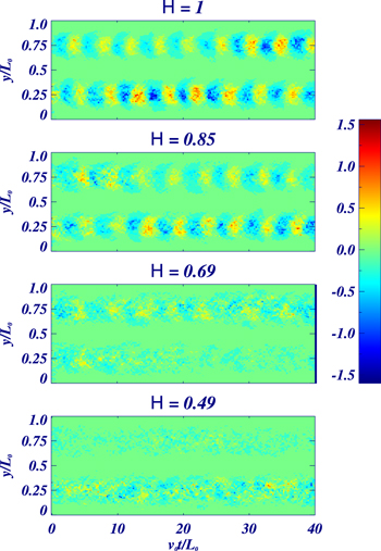
Figure 2. Bx (at z = 0) averaged over the x-direction as a function of t and y from four different simulations. We keep vs = 4, u0 while we vary  .
.
Download figure:
Standard image High-resolution image
Figure 3. Regime diagram for kinematic solutions as a function of H and  . The triangles mark the values of H and the ratio of fluctuating velocity to the shear amplitude from the wave simulations. The plus signs mark the rest of the simulations (no wave).
Download figure:
Standard image High-resolution imageThe emergence of dynamo waves depends on the presence of both large-scale shear and a small-scale flow lacking reflexional symmetry, for which the helicity provides a useful measure. Figure 3 shows that for reasonable values of the shear and helicity, a decrease in the helicity of the flow can be made up for by a corresponding increase in the shear—and vice versa. Here, it is important to be clear about in what sense there is a large-scale dynamo wave. All spatial scales of the solution grow exponentially with a well-defined growth rate. However the large scales also display oscillatory behavior with a well-defined period and a coherent phase, whereas the small scales have no such phase coherence. This "definition" is important and will play a role later when we analyze the nonlinear solutions.
3.3. Nonlinear Solutions
The nonlinear problem is solved as an initial value problem; therefore some initial conditions must be selected. We choose the initial conditions so that the nonlinear state emerges from a kinematic evolution that we understand. We therefore select Lz = 0.64; for this box size, and depending weakly on the shear, the fastest growing kinematic modes have a wavelength in z that is close to half the size of the box (in the vertical direction). Once the fastest growing mode has established itself, it grows exponentially with a well-defined growth rate and eventually the Lorentz force becomes important and nonlinear effects saturate the exponential growth and lead to a stationary nonlinear state.
It is conceivable that, and indeed it would be nice if, the process of saturation were associated with a slight change in the velocity, so that the overall morphology of the velocity and the magnetic field remains close to that of the kinematic phase, except that the magnetic field does not grow exponentially any more. This "weakly nonlinear" type of solution has not been found here (despite extensive investigations). Instead, what has been found is that the nonlinear saturation always involves significant modification of the velocity and a corresponding change in field morphology.
Typically, when the kinematic solution reaches a significant amplitude the system enters a complicated intermediate state and after a time—which can be a number of turnover times—we find that the solution takes one of four solution types. Before describing these we would like to make some general remarks concerning the underlying symmetries of the MHD system. The MHD equations only have quadratic nonlinearities that introduce certain symmetries that are best described spectrally. There are two invariant subspaces of solutions under evolution of the MHD equations. The first, which we term Type 1, has solutions where the velocity only has kz even (normalized to the height of the box Lz) and the magnetic field has kz odd. The second (Type 2) has the wavenumber of both the magnetic field and velocity even. Initial conditions that have either of these symmetries are therefore preserved (owing to the symmetry of our forcing). For example, the kinematic modes are of Type 1, so a "weakly nonlinear" saturation would rely on the Type 1 subspace being stable. However we have found that, whatever the symmetry of the final state—discussed below—the intermediate state always involves a solution that has no particular symmetry. Another general consideration concerns the characteristic scale of the solutions in the invariant z-direction. In the kinematic regime it is set by the wavelength of the mode of maximum growth rate; in the nonlinear regime it appears to be set by the box size, i.e., the solution expands in z to fill the entire box. For instance for a box of height 0.64 where the kinematic solution consists of two copies of the fastest growing mode stacked on top of each other, the nonlinear solution, depending on its symmetry has a magnetic field with either kz = 0 or kz = 1.
Figure 4 shows the distribution of solution types as a function of Reynolds number and inverse shear parameter  , where
  is the rms value of the velocity fluctuations (i.e., the velocity minus the shear). We should stress that although vS is prescribed
  is not, and changes as the calculation progresses. The values quoted in Figure 4 correspond to those calculated in the nonlinear state. The magnetic Prandtl number is fixed to have the value 2.5. The different symbols correspond to different types of solutions. We begin by describing a vertical cut at moderate Re going from small to large shear (we shall refer to the different types of solutions by their symbol type).
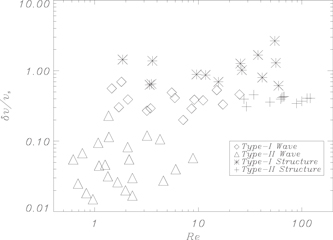
Figure 4. Regime diagram for nonlinear solutions (given in table 1). The values of  vs. Re are calculated in the nonlinear regime. We group them into four groups and assign each group with the following symbols: asterisk, diamond, triangle, and plus sign. Solutions in each group share the same properties.
Download figure:
Standard image High-resolution imageFigure 5 shows spacetime plots for three different types of solutions, where the two middle panels both correspond to diamonds. In the top panel there is no evidence of anything propagating. For every value of y the field is predominantly unidirectional and its direction rotates in the (z, x)-plane with y. In other words the large-scale field is in the form of a helix. It is interesting that, despite the time-dependent nature of the forcing, it is possible to find a solution that is nearly steady. Furthermore, we note that most of the magnetic energy is contained in a structure that does not react back on the velocity, does not interact with the shear, and dissipates very slowly. This is reminiscent of Archontis type dynamos (Archontis 2000; Cameron & Galloway 2006).

Figure 5. The averaged Bx over the x-direction as a function of t and y from four different simulations. We vary vs while keeping other parameters unchanged. From the top panel to the bottom panel, the magnitudes of vS are v0, 2v0, 4v0, and 8v0, respectively. The averaged values of δ v/vS are 1.4 (Run 14), 0.7 (Run 25), 0.3 (Run 39), and 0.1 (Run 60) in the same top-to-bottom order.
Download figure:
Standard image High-resolution imageEven though most of the magnetic energy is in the helical structure, it does have a weaker component with  . As the shear increases, the strength of this component increases relative to the helical structure and turns into a propagating wave. As shown in Figure 5 the helix itself may be unstable to an instability that wobbles it back and forth along the y-direction with a period that is much longer than that of the propagating wave. This wobbling appears to settle down with further increase of the shear as shown in Figure 5.
If the shear is further increased, the nature of the solution changes dramatically to a completely different morphology (triangle solutions). There is hardly any energy in the z-independent component of the magnetic field so the helix has gone and most of the structure is associated with true nonlinear propagating dynamo waves.
Information about the propagation speeds of the various solutions can be obtained from a cursory examination of Figure 6. It shows the time history of the phase of the propagating pattern. What is clear is that there are two propagation speeds, a slow one associated with the dynamo waves (triangles) and a fast one associated with the diamonds. In fact, by computing the slope, it is easy to verify that the propagating features in the diamond solutions are Alfvénic.
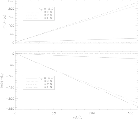
Figure 6. The values of  from the four simulations presented in Figure 5. The function ϕ(t) is from the assumption that the values of Bx are equal to
 ![$| {B}_{x}| \mathrm{exp}[{Re}(\phi (t))+i{\rm{Im}}(\phi (t))]$](https://content.cld.iop.org/journals/0004-637X/825/1/23/revision1/apjaa23f5ieqn36.gif) .
.
Download figure:
Standard image High-resolution imageThus far, we have increased the shear at fixed Re (and therefore Rm). However, when Re is increased for most values of vs, a radically different type of solution appears, corresponding to the + signs in Figure 4. We note that these solutions only appear in a small region of parameter space. For instance, these cannot be found for small values of  . This is not from lack of trying, rather because, even if kinematically the solution starts with low values of
  , it migrates to high values. These solutions at first glance do not appear to have any significant large-scale organization and may therefore be an example of small-scale dynamo action. However inspection of the time history of the magnetic energy reveals an episodic increase of the magnetic energy of the solutions (as shown in Figure 7). Interestingly these events correspond to a collapse to a solution with most of the energy in kz = 1. This is shown in Figure 7 where the two panels correspond to one of the disordered low energy states (A) and the other to the organized higher energy state (B). Remarkably, despite the fact that the forcing remains strongly helical, the "+" solution has no average helicity. Figure 8 shows how the averaged helicity drops to zero once the Lorentz force is no longer negligible.

Figure 7. The top panel shows the time evolution of magnetic energy for a typical "+" solution. The bottom left panel shows the color plot of Bx on the zy-plane at where magnetic energy is not at its peak, while the bottom right panel shows it at its peak. The simulation corresponds to Run 47.
Download figure:
Standard image High-resolution image
Figure 8. The time evolution of H as the function of time for the "+" solution shown in Figure 7. It rapidly drops to zero on average when the Lorentz force is no longer negligible.
Download figure:
Standard image High-resolution imageFigure 9 shows the spatial dependence of the helicity of the flow in the linear and nonlinear regimes. Interestingly the Lorentz force has had the effect of contracting strong helicity to a small fraction of the volume. Hence even though the helicity density may be large locally, the average helicity in the nonlinear regime is small. We stress that we believe this modification of the global helicity to be a dynamic effect, as it is apparent only when the Lorentz force has become significant.

Figure 9. Plot of the helicity density in the linear regime (left) and nonlinear regime (right) for the "+" solution of Figure 8.
Download figure:
Standard image High-resolution image
4. DISCUSSION AND CONCLUSION
In this paper, we have considered the problem of large-scale dynamo action in the nonlinear regime, with particular emphasis on the existence of nonlinear propagating dynamo waves. At this point in the investigation, we felt it was appropriate to look at a highly idealized system. Partly this was due to the need to construct a computationally feasible model; one that was compatible with a broad exploration of parameter space. More importantly the design was inspired by the "suppression principle," namely that at high Rm a large-scale dynamo will only be seen if some mechanism operates to suppress the fluctuations. Given the idealized nature of the model, it behooves us to discuss which features are robust and will continue to apply in other less idealized systems.
As noted by Tobias & Cattaneo (2015) a critical parameter in identifying whether a dynamo calculation is in the astrophysically relevant regime is the dynamo supercriticality parameter given by  . They argued that it is only when χ is sufficiently large (of the order of tens or hundreds) that the kinematic dynamo enters a regime where the growth rate becomes largely independent of Rm and the role of shear is then to suppress the small-scale dynamo. In that paper and in Tobias & Cattaneo (2013) and Cattaneo & Tobias (2014), because of the two-dimensional nature of the calculation, it was possible to reach χ ∼ 103. In the nonlinear regime it is difficult to reach high Rm—although we stress here that the dynamos considered here are designed to have small Rmc and for this reason we are able to reach
  , which we believe is significantly larger than for many other three-dimensional dynamo calculations.
Our main findings are that for a wide range of parameters, nonlinear large-scale dynamo action is possible. For some of these parameters the solutions indeed take the form of propagating dynamo waves. Moreover, the saturated nonlinear states are invariably very different from the kinematic ones. All the solutions with large-scale behavior had a vertical extent that was determined by the box size. Finally, at high enough Re and Rm the solutions cease to display any systematic behavior.
The vertical collapse of the solutions to the box size and the fact that at high Rm no solutions display systematic behavior are related to the design of our model. The first of these is due to the fact that, for our choice of the forcing, the equations have no characteristic scale in z and the equations are completely homogeneous (in that direction). The second is due to the inability of our type of forcing to continue to maintain a strongly helical flow at high Re. We anticipate that things may be very different in a system where the forcing is correlated with the velocity, for example in a rotating system where the Coriolis force, which may contribute to the generation of helical states, is linearly related to the velocity.
The physical reason for the transition between various states is difficult to characterize here. We stress that these solutions are extremely nonlinear, in the sense that they are far from the critical value of Rm for dynamo action. In this strongly nonlinear regime, the presence of a number of nonlinear states with different properties and the abrupt transition between them as a parameter is varied is not surprising. These bifurcations are usually associated with either the loss of stability of a specific configuration or, in certain cases, the loss of the state itself. Physically, the presence of dynamo waves for large values of the shear, however, can be ascribed to a weakening of the nonlinearity. In this regime where the shear is stronger, the system is better described by a quasilinear theory (see for example Squire & Bhattacharjee 2015 for such a theory applied to accretion disk turbulence)
We finish by commenting on the properties of the solutions that we believe to be robust. We believe that the dramatic differences between the kinematic and nonlinear states is not peculiar to this model, but probably applies in general. Unless Rm is small, saturation of a dynamo in a state similar to that from kinematic theory is the exception rather than the rule. In general the nonlinear states will be very different from the kinematic ones. Finally, we believe that the "suppression principle" is a useful guiding idea. We note that the dynamo waves in the nonlinear regime were smoother than those found in the kinematic regime—indicating that the Lorentz force has aided in suppressing the fluctuations in the dynamo.
APPENDIX A
It is obvious from Equation (5) that the forcing is specified once a prescription is given for the functions  . Here
  is given by

Conceptually it is easier to describe how these functions are generated in phase space (i.e., in terms of the Fourier transform of  ) which is what is actually used by the spectral code. In phase space the components of
  correspond to the locations where the Fourier amplitude is stored, and
  is completely determined once these complex values are prescribed. The real and imaginary parts of these are randomly chosen from a uniform distribution between
  and
and  . Amax is a function of k given by Amax = A0/k so that the spectrum is flat. A0 is chosen so that the resulting velocity in the kinematic regime is of
  (and is therefore a function of Re). These values are refreshed on average every turnover time,
  , for that specific
  . This is achieved as follows: every timestep a random number R between 0 and 1 is picked from a uniform distribution. If
  where
where  is the timestep, the values are refreshed; otherwise they are left unchanged.
: APPENDIX B
In this appendix we provide a table (Table 1) of the simulation runs performed and the resulting solutions.
Table 1. Simulation Parameters
| Run No. | Vs | η | A0 |

|

|
Re |

|
Phase Speed | Sol Type |
|---|---|---|---|---|---|---|---|---|---|
| 1 | 0.5 | 0.01 | 1.0 | 0.56 | 0.5 | 1.46 | 7.69 | 0.27 |

|
| 2 | 1.0 | 0.002 | 0.25 | 0.2 | 0.26 | 7.14 | 5.39 | 0.22 |

|
| 3 | 1.0 | 0.002 | 0.5 | 0.29 | 0.51 | 8.6 | 6.71 | 0.52 |

|
| 4 | 1.0 | 0.002 | 1.0 | 0.53 | 0.91 | 15.08 | 7.04 | 0.61 |

|
| 5 | 1.0 | 0.002 | 2.5 | 1.02 | 1.74 | 26.3 | 7.79 | N/A | * |
| 6 | 1.0 | 0.002 | 5.0 | 1.67 | 2.91 | 37.72 | 8.85 | N/A | * |
| 7 | 1.0 | 0.002 | 10.0 | 2.65 | 4.44 | 54.69 | 9.7 | N/A | * |
| 8 | 1.0 | 0.004 | 1.0 | 0.41 | 0.68 | 5.93 | 6.92 | 0.74 |

|
| 9 | 1.0 | 0.004 | 2.5 | 0.87 | 1.51 | 11.75 | 7.38 | N/A | * |
| 10 | 1.0 | 0.01 | 1.0 | 0.23 | 0.96 | 1.36 | 6.9 | 3.9 × 10⁻² | △ |
| 11 | 1.0 | 0.01 | 1.5 | 0.39 | 0.48 | 2.09 | 7.39 | 0.55 |

|
| 12 | 1.0 | 0.01 | 2.5 | 0.63 | 0.95 | 3.39 | 7.39 | N/A | * |
| 13 | 1.0 | 0.02 | 10.0 | 1.38 | 2.19 | 3.6 | 7.67 | N/A | * |
| 14 | 1.0 | 0.04 | 16.0 | 1.44 | 2.06 | 1.86 | 7.74 | N/A | * |
| 15 | 2.0 | 0.002 | 0.5 | 0.31 | 0.5 | 29.2 | 4.24 | N/A | + |
| 16 | 2.0 | 0.002 | 2.5 | 0.46 | 0.77 | 24.98 | 7.33 | 0.96 |

|
| 17 | 2.0 | 0.002 | 10.0 | 1.29 | 2.16 | 56.01 | 9.21 | N/A | * |
| 18 | 2.0 | 0.002 | 5.0 | 0.80 | 1.33 | 41.48 | 7.79 | N/A | * |
| 19 | 2.0 | 0.004 | 2.5 | 0.38 | 0.64 | 11.12 | 6.86 | 1.15 |

|
| 20 | 2.0 | 0.01 | 1.0 | 0.09 | 0.65 | 1.08 | 7.24 | 3.4 × 10⁻² | △ |
| 21 | 2.0 | 0.01 | 2.5 | 0.27 | 0.39 | 3.19 | 6.82 | 0.79 |

|
| 22 | 2.0 | 0.01 | 5.0 | 0.49 | 0.76 | 5.54 | 7.06 | 1.42 |

|
| 23 | 2.0 | 0.01 | 10.0 | 0.89 | 1.52 | 9.61 | 7.37 | N/A | * |
| 24 | 2.0 | 0.02 | 10.0 | 0.65 | 0.97 | 3.53 | 7.37 | N/A | * |
| 25 | 2.0 | 0.04 | 16.0 | 0.70 | 0.67 | 1.81 | 7.66 | 1.45 |

|
| 26 | 4.0 | 0.002 | 0.25 | 0.04 | 0.34 | 6.05 | 5.35 | 9.7 × 10⁻³ | △ |
| 27 | 4.0 | 0.002 | 0.5 | 0.4 | 0.4 | 62.49 | 5.07 | N/A | + |
| 28 | 4.0 | 0.002 | 1.0 | 0.42 | 0.35 | 63.96 | 5.23 | N/A | + |
| 29 | 4.0 | 0.002 | 2.5 | 0.36 | 0.38 | 49.21 | 5.86 | N/A | + |
| 30 | 4.0 | 0.01 | 0.5 | 0.03 | 0.28 | 0.69 | 5.91 | 1.7 × 10⁻² | △ |
| 31 | 4.0 | 0.01 | 1.0 | 0.05 | 0.39 | 1.10 | 6.41 | 3. × 10−2 | △ |
| 32 | 4.0 | 0.01 | 2.0 | 0.08 | 0.59 | 2.08 | 6.41 | 4.2 × 10⁻² | △ |
| 33 | 4.0 | 0.01 | 10.0 | 0.39 | 0.6 | 9.15 | 6.78 | 2.37 |

|
| 34 | 4.0 | 0.01 | 20.0 | 0.7 | 1.09 | 15.63 | 7.13 | N/A | * |
| 35 | 4.0 | 0.01 | 40.0 | 1.26 | 2.14 | 25.49 | 7.92 | N/A | * |
| 36 | 4.0 | 0.02 | 2.0 | 0.06 | 0.35 | 0.62 | 7.09 | 6.1 × 10⁻² | △ |
| 37 | 4.0 | 0.02 | 2.5 | 0.07 | 0.42 | 0.76 | 7.10 | 6.6 × 10⁻² | △ |
| 38 | 4.0 | 0.02 | 10.0 | 0.29 | 1.59 | 3.46 | 6.76 | 1.49 |

|
| 39 | 4.0 | 0.04 | 16.0 | 0.30 | 0.36 | 1.71 | 7.10 | 1.34 |

|
| 40 | 6.0 | 0.01 | 0.5 | 0.018 | 0.26 | 0.83 | 5.37 | 1.3 × 10⁻² | △ |
| 41 | 6.0 | 0.01 | 1.0 | 0.032 | 0.34 | 1.34 | 5.64 | 2.2 × 10⁻² | △ |
| 42 | 6.0 | 0.01 | 2.0 | 0.055 | 0.46 | 2.15 | 6.10 | 4.2 × 10⁻² | △ |
| 43 | 6.0 | 0.01 | 4.0 | 0.11 | 0.58 | 4.27 | 6.00 | 6.5 × 10⁻² | △ |
| 44 | 8.0 | 0.002 | 0.1 | 0.37 | 0.43 | 99.70 | 5.97 | N/A | + |
| 45 | 8.0 | 0.002 | 0.5 | 0.41 | 0.70 | 120.45 | 5.41 | N/A | + |
| 46 | 8.0 | 0.002 | 1.0 | 0.41 | 0.58 | 112.38 | 5.79 | N/A | + |
| 47 | 8.0 | 0.002 | 2.5 | 0.34 | 0.39 | 88.7 | 6.21 | N/A | + |
| 48 | 8.0 | 0.004 | 0.5 | 0.028 | 0.31 | 4.60 | 4.82 | 9.4 × 10⁻³ | △ |
| 49 | 8.0 | 0.004 | 1.0 | 0.43 | 0.37 | 67.43 | 5.10 | N/A | + |
| 50 | 8.0 | 0.004 | 2.5 | 0.43 | 0.33 | 65.95 | 5.19 | N/A | + |
| 51 | 8.0 | 0.008 | 1.0 | 0.015 | 0.33 | 2.31 | 5.19 | 1.9 × 10⁻² | △ |
| 52 | 8.0 | 0.01 | 0.5 | 0.031 | 0.23 | 0.96 | 5.10 | 8.6 × 10⁻³ | △ |
| 53 | 8.0 | 0.01 | 1.0 | 0.026 | 0.31 | 1.66 | 5.13 | 1.8 × 10⁻² | △ |
| 54 | 8.0 | 0.01 | 5.0 | 0.46 | 0.27 | 34.23 | 4.27 | N/A | + |
| 55 | 8.0 | 0.01 | 2.5 | 0.058 | 0.41 | 3.6 | 5.14 | 4.3 × 10⁻² | △ |
| 56 | 8.0 | 0.01 | 10.0 | 0.40 | 0.30 | 27.59 | 4.59 | N/A | + |
| 57 | 8.0 | 0.01 | 20.0 | 0.33 | 0.45 | 17.28 | 6.14 | 1.13 |

|
| 58 | 8.0 | 0.02 | 3.5 | 0.046 | 0.37 | 1.26 | 5.86 | 5.8 × 10⁻² | △ |
| 59 | 8.0 | 0.02 | 10.0 | 0.12 | 0.62 | 3.20 | 5.98 | 0.10 | △ |
| 60 | 8.0 | 0.04 | 16.0 | 0.12 | 0.64 | 1.37 | 6.70 | 0.15 | △ |
| 61 | 12.0 | 0.01 | 1.0 | 0.02 | 0.27 | 1.98 | 4.84 | 1.4 × 10⁻² | △ |
| 62 | 16.0 | 0.01 | 1.0 | 0.017 | 0.25 | 2.31 | 4.68 | 9.3 × 10⁻³ | △ |
Download table as: ASCIITypeset image