


ABSTRACT
The distribution of helium in the intracluster medium (ICM) permeating galaxy clusters is not well constrained due to the very high plasma temperature. Therefore, the plasma is often assumed to be homogeneous. A nonuniform helium distribution can, however, lead to biases when measuring key cluster parameters. This has motivated one-dimensional models that evolve the ICM composition assuming that the effects of magnetic fields can be parameterized or ignored. Such models for nonisothermal clusters show that helium can sediment in the cluster core, leading to a peak in concentration offset from the cluster center. The resulting profiles have recently been shown to be linearly unstable when the weakly collisional character of the magnetized plasma is considered. In this paper, we present a modified version of the MHD code Athena, which makes it possible to evolve a weakly collisional plasma subject to a gravitational field and stratified in both temperature and composition. We thoroughly test our implementation and confirm excellent agreement against several analytical results. In order to isolate the effects of composition, in this initial study we focus our attention on isothermal plasmas. We show that plasma instabilities, feeding off gradients in composition, can induce turbulent mixing and saturate by rearranging magnetic field lines and alleviating the composition gradient. Composition profiles that increase with radius lead to instabilities that saturate by driving the average magnetic field inclination to roughly 45°. We speculate that this effect may alleviate the core insulation observed in homogeneous settings, with potential consequences for the associated cooling flow problem.
Export citation and abstract BibTeX RIS
1. INTRODUCTION
Atmospheres composed of a plasma that is weakly collisional and weakly magnetized have stability properties that differ qualitatively from collisional atmospheres. Instabilities such as the magnetothermal instability (MTI; Balbus 2000, 2001) and the heat-flux-driven buoyancy instability (HBI; Quataert 2008) can arise when there is a gradient in the temperature either parallel or anti-parallel to the gravitational field. These instabilities, which feed off a gradient in temperature, have been extensively studied (Balbus 2000, 2001; Parrish & Stone 2005, 2007; Parrish & Quataert 2008; Parrish et al. 2008, 2009, 2010, 2012a, 2012b; Quataert 2008; Bogdanović et al. 2009; Ruszkowski & Oh 2010; Kunz 2011; McCourt et al. 2011, 2012; Kunz et al. 2012; Latter & Kunz 2012), and they are believed to be important for the understanding of the dynamical evolution of the intracluster medium (ICM) of galaxy clusters.
These studies assumed that the composition of the plasma is uniform, an assumption that might not be appropriate if heavier elements are able to sediment toward the core of the cluster (Fabian & Pringle 1977). In parallel and complementary studies, the long-term evolution of the radial distribution of elements has been studied using one-dimensional models (Fabian & Pringle 1977; Gilfanov & Syunyaev 1984; Chuzhoy & Nusser 2003; Chuzhoy & Loeb 2004; Peng & Nagai 2009; Shtykovskiy & Gilfanov 2010). The ensuing nonuniform composition has been argued to introduce biases in cluster properties as inferred from observations (Markevitch 2007; Peng & Nagai 2009).
While the studies of the MTI and HBI assumed a uniform plasma, the sedimentation models have yet to include magnetic fields. In an attempt to bridge the gap between the different approaches, and with the goal of understanding the long-term evolution of the composition of the ICM, Pessah & Chakraborty (2013) studied the stability properties of weakly collisional atmospheres with gradients in both temperature and composition. They found that gradients in composition, either parallel or anti-parallel to the gravitational field, can trigger instabilities. In a subsequent study, Berlok & Pessah (2015) carried out a comprehensive study using linear mode analysis and showed that these instabilities are expected to render the composition profiles obtained with current sedimentation models unstable, as it was illustrated using the model of Peng & Nagai (2009).
In this paper, we present the first nonlinear, two-dimensional (2D), numerical simulations of the instabilities that feed off a gradient in composition using a modified version of the MHD code Athena (Stone et al. 2008). The instabilities considered are (i) the magneto-thermo-compositional instability (MTCI), which is maximally unstable when the magnetic field is perpendicular to gravity; (ii) the heat- and particle-flux-driven buoyancy instability (HPBI), which is maximally unstable when the magnetic field is parallel to gravity; and (iii) the diffusion modes, which are maximally unstable when the magnetic field is parallel to gravity. These instabilities arise due to the weakly collisional nature of the ICM, which fundamentally changes the transport properties of a plasma. In this regime, where the gyro-radii of the particles are much smaller than the mean free path for particle collisions, the transport of heat, momentum, and particles will be primarily along the magnetic field lines.
The MTCI and HPBI will be present in isothermal atmospheres in which the composition increases with height, while diffusion modes can be present regardless of the direction of the gradient in composition (Pessah & Chakraborty 2013). The linear dispersion relation presented in Berlok & Pessah (2015) is used to compare with the linear evolution of the simulations. We find good agreement, thereby confirming both the linear theory and our numerical method. For the nonlinear evolution of the instabilities we find that the magnetic field inclination goes to roughly 45° independently of whether the magnetic field is initially horizontal (MTCI) or vertical (HPBI). This is contrary to the instabilities driven by temperature gradients, where the average magnetic field becomes almost vertical (horizontal) for an initially horizontal (vertical) magnetic field (Parrish & Stone 2005; Parrish & Quataert 2008). The simple explanation is that the MTCI and HPBI, both of which grow when the composition increases with height, can operate simultaneously. They are therefore driving the average angle in opposite directions, compromising at roughly 45°. The MTI and HBI, being dependent on temperature gradients in opposite directions, cannot grow at the same time, and so they grow unabated by their counterpart. We also find that both types of instabilities cause turbulent mixing of the helium concentration. We conclude that, in the idealized numerical settings that we employ, instabilities driven by the free energy supplied by a gradient in composition saturate by alleviating the gradient and thereby removing the source of free energy.
The rest of the paper is organized as follows: we start out by introducing the equations of kinetic MHD in Section 2 and how they can be solved numerically in Section 3. In Section 4 we demonstrate that the simulations agree with the linear theory for isothermal atmospheres, and we illustrate how the growth rates depend on some of the key parameters of the problem. We also use atmospheres with gradients in both temperature and composition, motivated by the model of Peng & Nagai (2009) and discussed in Berlok & Pessah (2015), to show that the theory and simulations also agree with both gradients present. In Section 5, we consider the nonlinear evolution of the MTCI and HPBI in isothermal atmospheres in order to determine how they saturate. We summarize and outline future work in Section 6.
2. KINETIC MHD FOR A BINARY MIXTURE
We consider a fully ionized, weakly magnetized, and weakly collisional plasma consisting of a mixture of hydrogen and helium. We model such a plasma using the set of equations introduced in Pessah & Chakraborty (2013),1


In these equations ρ is the mass density,  is the fluid velocity,
  is the magnetic field with direction
  is the gravitational acceleration, and
  is the identity matrix. The total pressure is
  , where P is the thermal pressure and the total energy density, E, is

where  is the adiabatic index.
The composition of the plasma, c, is defined to be the ratio of the helium density to the total gas density

and the associated mean molecular weight, μ, is given by

for a completely ionized plasma consisting of helium and hydrogen. The mean molecular weight can modify the dynamics of the plasma through the equation of state

where  is Boltzmann's constant, T is the temperature, and
  is the proton mass.
We consider the plasma to be influenced by three different nonideal effects: Braginskii viscosity, which arises due to differences in pressure parallel ( ) and perpendicular (
 ) to the magnetic field, described by the viscosity tensor (Braginskii 1965)

anisotropic heat conduction described by the heat flux (Spitzer 1962; Braginskii 1965),

and anisotropic diffusion of composition described by the composition flux (Bahcall & Loeb 1990),

The transport coefficients for Braginskii viscosity ( ), heat conductivity (
 ), and diffusion of composition (D) depend on the temperature, density, and composition of the plasma. The dependences are given by Equations (64)–(66) in Berlok & Pessah (2015). Finally, we define the thermal velocity,
  , and the plasma-β given by
  where
where  is the Alfvén velocity.2
3. NUMERICAL METHOD AND INITIAL CONDITIONS
The equations of kinetic MHD, Equations (1)–(5), are solved using a modified version of the conservative MHD code Athena (Stone et al. 2008). The algorithms used in Athena are described in Gardiner & Stone (2005) and Stone & Gardiner (2009), and a description of the implementation of anisotropic thermal conduction and Braginskii viscosity can be found in Parrish & Stone (2005) and Parrish et al. (2012b), respectively.
In order to carry out the numerical simulations of interest, we have modified Athena to include a spatially varying mean molecular weight, μ. This is done by using the inbuilt method for adding a passive scalar, defined by a spatially varying concentration, c, and then making it active by using the value of c when calculating the temperature used in the heat conduction module. Furthermore, we implemented a module that takes account of diffusion of helium by using operator splitting. This module has been built by following the same approach employed in the heat conduction module that is already present in the current publicly available version of Athena (Parrish & Stone 2005; Sharma & Hammett 2007). Our implementation allows for nonconstant values of the parameters  , and D through user-defined functions. This feature is, however, not used in this work, as we employ a local approximation and thus treat these parameters as constants. The diffusion terms are solved explicitly, which can make the time-step constraint on viscosity, thermal conduction, and diffusion of helium very restrictive. In order to circumvent this, we use subcycling, which we limit to a maximum of 10 steps per MHD step (Kunz et al. 2012).
3.1. Plane-parallel Atmosphere with Gradients in Temperature and Composition
In this section, we introduce the two different atmospheres used as initial conditions in the simulations. The atmospheres considered are plane-parallel, i.e., all quantities are constant along a horizontal slice, perpendicular to gravity. The atmosphere is assumed to be composed of an ideal gas, characterized by the equation of state given by Equation (9), and is assumed to be in hydrostatic equilibrium, i.e.,3

3.1.1. Isothermal Atmosphere with a Composition Gradient in the Absence of Particle Diffusion
The simplest atmosphere we use is inspired by the original numerical work on the MTI (Parrish & Stone 2005). We consider an isothermal atmosphere with  and
and


where  , and
, and  are the values of the pressure, temperature, and mean molecular weight at z = 0, respectively, and H0 is the scale height

The density can be determined using Equation (9).
This isothermal atmosphere is used for simulations of the linear regime of the MTCI in Section 4.1 and the linear regime of the HPBI in Section 4.2. It is also used for simulations of the nonlinear regime of the MTCI and HPBI in Section 5. The magnetic field can have any orientation as long as D = 0. The structure of this atmosphere is, however, not in equilibrium if  and
and  . In that case, we will have to use a more sophisticated atmosphere, which we introduce next.
3.1.2. Atmosphere with Thermal and Composition Gradients
Steady state requires that the divergence of the heat and particle fluxes vanish, i.e.,


Both conditions are trivially satisfied if bz = 0 and D = 0. If, however,  and
and  , these requirements can still be met by simple atmospheric models if
  and D do not depend on z. Such an assumption is reasonable for the local simulations that we will consider, where the height of the box, Lz, satisfies the criterion
  . When there is both a gradient in temperature T and mean molecular weight μ, the requirements that
  and
and  can be integrated to yield


where  and
and  are the constant slopes in temperature and composition. Here T0 (
 ) is the temperature at the bottom (top) of the box and c0 (
 ) is the helium mass concentration at the bottom (top) of the box.
The pressure is found by solving Equation (13), leading to

where  is related to c(z) by Equation (8) and the constant α is given by

This solution for the pressure profile of the atmosphere is replaced with a simple exponential atmosphere,  , with scale height H0 if
  .
.
We use this model atmosphere to perform simulations of modes driven by diffusion in Section 4.3. These modes are unstable when there is a vertical gradient in composition, a nonzero vertical component of the magnetic field,  , and anisotropic diffusion of helium, D
  0. We also use this atmosphere in Section 4.4 for simulations of the linear regime of the MTCI and the HBPI with gradients in both temperature and composition.
3.2. Boundary Conditions
Periodic boundary conditions are used in the horizontal direction in all simulations. In the vertical direction we have implemented two different sets of boundary conditions: (i) the conventional reflective boundary conditions and (ii) a set of boundary conditions that we will call quasi-periodic boundary conditions. Both sets of boundary conditions are explained in detail in Appendix
The quasi-periodic boundary conditions are periodic in the relative changes in the physical quantities. We have found that these boundary conditions are a necessity in order for the simulations to reproduce the growth rates predicted by the local linear mode analysis. We believe that this is due to the assumption of periodicity in the perturbed quantities that is made when the dispersion relation is derived. This problem has also been encountered in previous studies of the MTI (Rasera & Chandran 2008). These boundary conditions are used in all simulations presented in Section 4.
The reflective boundary conditions maintain hydrostatic equilibrium by extrapolating pressure and density into the ghost zones at the top and bottom of the computational domain. The values of temperature and composition are held fixed at their initial values in the ghost zones. The velocity z-component is reflected symmetrically around the boundaries. If the magnetic field is initially vertical (horizontal), it is forced to remain vertical (horizontal) at the boundaries. These boundary conditions are used in the simulations presented in Section 5.
4. SIMULATIONS OF THE LINEAR REGIME
The equations are made dimensionless by scaling the density with  , distances with H0, and velocities with the thermal velocity
  . The magnetic field strength B0 is found from the dimensionless parameter
  . Here the subscript "0" denotes the value at the bottom of the computational domain, z = 0. With this convention, the unit of time is
  , temperature is scaled with
  is scaled with
  , pressure, as well as energy density, is scaled with
  , and the value of g is unity. As a consequence, the coefficient for anisotropic heat conduction,
  , is scaled with
  , and the coefficients for Braginskii viscosity
 , and anisotropic diffusion of composition, D, are both scaled with
  .
.
We begin by comparing the simulations with the linear theory. In order to do so, we use the quasi-periodic boundary conditions described in the previous section and in Appendix ![$[0,{L}_{x}]\times [0,{L}_{z}]$](https://content.cld.iop.org/journals/0004-637X/824/1/32/revision1/apj523632ieqn48.gif) with
with  and a resolution of 64 × 64 is used in all simulations unless otherwise noted. An overview of the simulations of the linear regime can be found in Table 1.
Table 1. Simulations of the Linear Regime Using Quasi-periodic Boundary Conditions
| Simulation | ( ) ) |
θ |

|

|

|
D | Resolution | Figure |
|---|---|---|---|---|---|---|---|---|
| MTCI_chi | (1, 0) | 0° | 2 × 10⁸ | ⋯ | 0 | 0 | 64 × 64 | 3(a) |
| MTCI_B |

|
0° | ⋯ | 3 × 10⁻⁴ | 0 | 0 | 64 × 64 | 3(b) |
| HPBI_nu |

|
90° | 2 × 10⁸ | 10−4 | ⋯ | 0 | 64 × 64 | 4(a) |
| HPBI_n | (⋯, ⋯) | 90° | 2 × 10⁶ | 10−4 | 0 | 0 | 256 × 256 | 4(b) |
| D-mode_D |

|
90° | 2 × 10⁸ | 10−3 | 0 | ⋯ | 256 × 256 | 5(a) |
| D-mode_nu |

|
90° | 2 × 10⁸ | 10−3 | ⋯ | 10−3 | 64 × 64 | 5(b) |
| MTCI_ICMa | (⋯, 0) | 0° | 2 × 10⁶ |

|

|
0 | 256 × 32 | 6(a) |
| HPBI_ICMa | (⋯, ⋯) | 90° | 2 × 10⁶ |

|

|
0 | 256 × 256 | 6(b) |
Note. Each row represents a series of simulations, where the ellipses denote that the associated parameter is being varied.
aUsing gradients in both temperature and composition.Download table as: ASCIITypeset image
The instabilities are excited by seeding a given mode, with components ( ), as derived by solving the eigenvalue system associated with the dispersion relation introduced in Pessah & Chakraborty (2013) and Berlok & Pessah (2015). We set the overall mode amplitude by enforcing
  , so that the velocity perturbation is subsonic (Parrish & Stone 2005). The amplitudes of the other components are fixed by the solution to the linear eigenvalue problem, which predicts that unstable modes grow exponentially as
  while the ratio of their components remains constant in time.
We begin by considering D = 0 and the hydrostatic atmosphere given in Section 3.1.1, which has  and
and  . This atmosphere is unstable regardless of whether the magnetic field is oriented horizontally (MTCI) or vertically (HPBI), as described in Berlok & Pessah (2015).
4.1. The Magneto-thermo-compositional Instability
When the magnetic field is perpendicular to gravity, the general dispersion relation, Equation (13) in Berlok & Pessah (2015), reduces to

in the limit of fast heat conduction and weak magnetic field. When  increases with height and the atmosphere is isothermal, we have
  . This is the instability known as the MTCI (Pessah & Chakraborty 2013). In order to excite a single MTCI mode, we use a perturbation of the form4
 and
and  . We are interested in a direct visual comparison of the spatial dependence of the perturbations in the simulations and the one expected from the linear theory. In order to illustrate this, we consider a setting with
  and
and  . In Figure 1, we show the values of the perturbations (green crosses)
  , and
, and  as a function of the x-coordinate. The data slices are drawn at a fixed height,
  at the time t = 5 in dimensionless units. The numerical results show good agreement with the analytical results shown with blue solid lines.
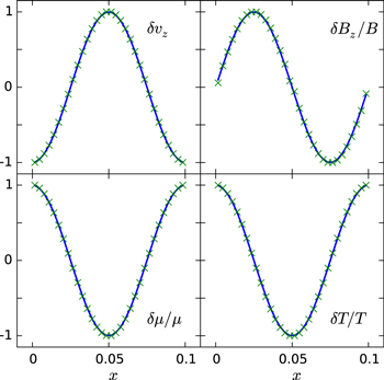
Figure 1. Four of the components of the perturbation at  for a mode with
  at time t = 5 in a simulation with resolution 32 × 32. The simulation (green crosses) matches the theory (blue lines). The magnetic field is
  out of phase with the velocity perturbation, as expected for a purely growing mode.
Download figure:
Standard image High-resolution imageIn order to calculate the growth rate of the mode, we perform an exponential fit to the time evolution of the box average of the absolute value of any of the perturbed quantities, which are shown in Figure 2. As expected from the local linear mode analysis, the amplitudes of the various components of the perturbation grow exponentially at the same rate.

Figure 2. Evolution of box-averaged quantities. The perturbed quantities grow exponentially with a growth rate  .
.
Download figure:
Standard image High-resolution imageThe growth rate of the MTCI depends on, among other things, the value of the heat conductivity,  , and the initial magnetic field strength, B0. In order to illustrate this dependence, and at the same time test our modification to the code, we perform a parameter study. In the left panel of Figure 3, we show how the growth rate increases with the value of the heat conductivity,
  . This is to be expected because the MTCI is driven by heat transfer along magnetic field lines. In the right panel of Figure 3, we show how the growth rate decreases with the value of
  . The explanation for this behavior is that magnetic tension tends to stabilize the MTCI (Berlok & Pessah 2015). Magnetic tension has stabilizing effects in the limit
  , where
  and
and  . In dimensionless units, this requirement can be written as
  . From this estimate, the growth rates shown in the right panel of Figure 3 should be negligible when
  . The simulations and the solution to the dispersion relation show that the growth rates are already inhibited by magnetic tension at lower values of
  . These examples were generated by running 10 simulations at a modest resolution (64 × 64). At this resolution the growth rates match to within a percent of the values expected from linear theory.

Figure 3. Growth rates for the MTCI. Left: the growth rate increases with the value of  . Right: the growth rate decreases with increasing initial magnetic field strength. The solid blue lines represent the theoretical values evaluated at
  . The green crosses are growth rates obtained from the simulations.
Download figure:
Standard image High-resolution image4.2. The Heat- and Particle-flux-driven Buoyancy Instability
When the magnetic field is parallel to gravity, the general dispersion relation reduces to

in the limit of fast heat conduction and weak magnetic field. The isothermal atmosphere where μ increases with height, which we considered in the previous section, is therefore also unstable when the magnetic field is vertical. In this case, the instability has been termed the HPBI (Pessah & Chakraborty 2013).
In this example, we include Braginskii viscosity, which inhibits the growth rate by damping perturbations perpendicular to the magnetic field. Braginskii viscosity can be important for the HPBI (Berlok & Pessah 2015). The mechanism is similar to the mechanism described by Kunz (2011) for the HBI. In order to excite a single mode of the HPBI, we use a perturbation with wavenumbers  and
and  , where
  is the mode number. We show the growth rate as a function of the Braginskii viscosity coefficient,
  in the left panel of Figure 4. These simulations used a fixed value of
  , and a numerical resolution of 64 × 64. As expected, the growth rate indeed decreases with increasing value of viscosity
  .
.

Figure 4. Growth rates for the local HPBI. Left: the growth rate decreases with the value of  . Right: the growth rate as a function of the mode number,
  . The solid blue lines represent the theoretical values evaluated at
  . The green crosses are growth rates obtained from the simulations.
Download figure:
Standard image High-resolution imageThe second dependence we study for the HPBI is the one on the mode number, n. High wavenumbers require higher numerical resolution in order to be resolved, and we use a resolution of 256 × 256 for these simulations. For the sake of simplicity, Braginskii viscosity is not included in these simulations. The result is shown in the right panel of Figure 4. The growth rate increases for increasing wavenumber because small wavelength perturbations have a shorter timescale for heat conduction. When the wavelength is too short, magnetic field tension renders the modes stable. A naive estimate, using  , suggests that this should happen when
  , but the exact solution to the dispersion relation shows that the instability is quenched already when n = 7. Using such simulations, we can directly see the cutoff in unstable wavenumbers resulting from magnetic field tension (as in this case) or viscosity (not shown here).
4.3. Modes Driven by Diffusion
One of the interesting findings of Pessah & Chakraborty (2013) is that there are instabilities that are driven by particle diffusion. This means that even though the equilibrium is stable according to Equation (24), the fact that  makes the equilibrium unstable. In order to study these unstable modes, we assume, for simplicity, an isothermal atmosphere with an initially vertical magnetic field.
In this case, as explained in Section 3.1, an equilibrium configuration needs to fulfill  , and so we consider the atmosphere given in Section 3.1.2 as an initial condition. According to Equation (24), this configuration is unstable to the HPBI for an isothermal atmosphere when the helium concentration increases vertically. If instead the helium concentration decreases with height, the atmosphere is stable in the absence of anisotropic particle diffusion. Choosing the slope in composition to be
  , we do not observe any instabilities in the simulation when D = 0. The situation changes dramatically, turning unstable when
  . The growth rates found in such simulations are compared with the predictions from the linear theory in Figure 5. Since the modes are driven by diffusion of helium, we expect the growth rate to increase with the value of D (left panel). The modes have a damped growth rate when Braginskii viscosity is included. We observe a decrease in the growth rate with increasing
  , in agreement with the solution to the dispersion relation (right panel).

Figure 5. Growth rate as a function of D (left) and  for fixed values of
  (right). The solid blue line represents the theoretical values evaluated at
  , and the green crosses are growth rates obtained from the simulations.
Download figure:
Standard image High-resolution image4.4. Gradients in Temperature and Composition
Having tested the case of isothermal atmospheres, we now consider a more general situation where both  and
and  . In order to work with sensible values for these gradients, we consider the models in Peng & Nagai (2009), who analyzed the long-term evolution of the concentration of helium in a one-dimensional setting by solving a coupled set of Burgers' equations for a multicomponent plasma in the absence of a magnetic field. Berlok & Pessah (2015) analyzed the stability of the Peng & Nagai (2009) model by focusing on local regions, characterized by fixed temperature and composition gradients, and modeling these as a plane-parallel atmosphere.
In this section, we present local simulations with gradients in temperature and composition estimated at  and
and  with
with  Mpc in the Peng & Nagai (2009) model. These are the locations that were analyzed in Sections 6.6 and 6.4 in Berlok & Pessah (2015), indicated with a C and an A in Figure 8 in that paper. These two locations correspond to the inner region where the temperature and composition increase with radius and the outer region where the temperature and composition decrease with radius. At these radii, the values for the logarithmic gradients are
  and
and  at
at  and
and  and
and  at
at  .
.
We use the equilibrium derived in Section 3.1.2 with values taken from the model of Peng & Nagai (2009),  (
( keV) and
  (
( ) for the inner (outer) region. The computational domain is
  where
where  kpc for the inner region and
  where
where  Mpc for the outer region. The gradients in composition and temperature are set such that the dimensionless values of
  and
and  in the plane-parallel atmosphere agree with the values in the model of Peng & Nagai (2009). They are given by
  Mpc−1 (
 Mpc−1) and
  kpc−1 (
 Mpc−1) for the inner (outer) region.
The values for  , and D are calculated from the model of Peng & Nagai (2009) as explained in the appendix of Berlok & Pessah (2015). The dimensionless values are so large that high-resolution numerical simulations become very computationally expensive. As this is a test, we have arbitrarily reduced the values by a factor of 100 in the simulations. We use a value of
  for both sets of simulations and adopt a resolution of 32 × 256 (MTCI) and 256 × 256 (HPBI). Some of the details of the simulations are listed in Table 1 with the names HPBI_ICM and MTCI_ICM. The growth rates also depend on the wavenumbers, kx and kz. For the HPBI (in the inner region) we take
  and investigate growth rate as a function of k. For the MTCI (in the outer region) we take kz = 0 and investigate the growth rate as a function of kx. The results are shown in Figure 6, with the growth rates of the HPBI in the left panel and the growth rates of the MTCI in the right panel. An estimate shows that the HPBI should be suppressed by magnetic tension for
  and the MTCI should be suppressed for
  . The growth rates are in units of 50 and 280 Myr, respectively. Therefore, in physical units, the maximum growth rates in these simulations are
  for the HBPI and
  for the MTCI.

Figure 6. Left: growth rates in the inner region as a function of  . Right: growth rates in the outer region as a function of kx for kz = 0. The solid blue line represents the theoretical values evaluated at
  , and the green crosses are growth rates obtained from the simulations.
Download figure:
Standard image High-resolution image5. SIMULATIONS OF THE NONLINEAR REGIME
In order to study the nonlinear evolution of the MTCI and the HPBI, we use the reflective boundaries described in Appendix  . We use a value of 2 × 10⁸ for the plasma-β. An overview of the simulations of the nonlinear regime can be found in Table 2.
Table 2. Overview of the Simulations of the Nonlinear Regime Using the Reflective Boundary Conditions
| Simulation | θ |

|

|

|
D | Resolution | Figure |
|---|---|---|---|---|---|---|---|
| MTCI256 | 0° | 2 × 10⁸ | 5 × 10⁻⁴ | 0 | 0 | 256 × 256 | 7(a), 8, 10 |
| HPBI128 | 90° | 2 × 10⁸ | 5 × 10⁻⁴ | 0 | 0 | 128 × 128 | 9 |
| HPBI256 | 90° | 2 × 10⁸ | 5 × 10⁻⁴ | 0 | 0 | 256 × 256 | 9 |
| HPBI512 | 90° | 2 × 10⁸ | 5 × 10⁻⁴ | 0 | 0 | 512 × 512 | 7(b), 9, 10 |
Download table as: ASCIITypeset image
We start out by studying the evolution of the MTCI, i.e., we consider an atmosphere threaded by a horizontal magnetic field. The subsequent evolution of the magnetic field and the plasma composition is illustrated in the upper panel of Figure 7. In this figure, it is evident that the MTCI is able to mix the helium content and to completely rearrange the initially ordered magnetic field. The resulting growths in kinetic and magnetic energy densities are shown, respectively, in the left and right panels of Figure 8. The kinetic energies associated with the two velocity components are roughly in equipartition throughout the simulation, i.e.,  with
with  always larger but never exceeding
  by more than an order of magnitude. The exponential phase of the instability ends at
  . After this point in time, both the kinetic and magnetic energies saturate, with the former exceeding the latter by two orders of magnitude. In spite of the fact that
  vanishes initially, by the end of the simulation the energies associated with the two magnetic field components are roughly in equipartition with
  larger than
  by a factor of
  , with
  having grown by a factor of
  with respect to its initial value.
Download figure:
Video Standard image High-resolution imageFigure 7. Evolution of instabilities in an isothermal atmosphere with  . The magnetic field lines are shown as solid black lines. The composition of the plasma is shown with green representing a high concentration and purple representing a low concentration. The MTCI (upper panel) and the HPBI (lower panel) both give rise to mixing of the helium content. The size of the computational domain is
  . The motions generated by the instabilities can be hinted at by comparing neighboring snapshots but are best understood from the animated version of this figure (see the online version).
Download figure:
Video Standard image High-resolution image
Figure 8. Evolution of kinetic (left panel) and magnetic (right panel) energies for the MTCI. After the initial phase of exponential growth, the instability saturates with energies that are roughly in equipartition.
Download figure:
Standard image High-resolution imageWe now consider the evolution of the HPBI. The setup is essentially the same, but the initial magnetic field is now vertical.5
The evolution of the HPBI is illustrated in the lower panel of Figure 7 with a resolution of 512 × 512. The initial vertical magnetic field is rearranged by the HPBI, and, as for the MTCI, the helium content is mixed by the action of the instability. The HPBI leads to growth in the magnetic and kinetic energy densities. In order to asses whether this growth is numerically converged, we have also run simulations at resolutions of 128 × 128 and 256 × 256. We show the evolution of  and
and  for the three different numerical resolutions in Figure 9. We observe that the instability leads to exponential growth followed by saturation in both
  and
and  . While the growth rate increases with increasing resolution, the values in the saturated state agree quite well.
Figure 9. Convergence of  and
and  as a function of resolution. The highest resolution is much more expensive to run because of the prohibitive time step constraint due to heat conduction; see Appendix
Download figure:
Standard image High-resolution imageIt is also of interest to understand how the magnetic field changes from being initially vertical to having a large horizontal component because the magnetic field inclination has consequences for heat transport along the vertical direction of the box. Such studies have been done for both the MTI (Parrish & Stone 2005, 2007) and the HBI (Parrish & Quataert 2008). These studies were motivated by a need to understand the cooling flow problem of galaxy clusters (Fabian 1994), and whether magnetic fields could alleviate this problem. While the MTI could potentially increase heat transport toward the core by making the magnetic field be preferentially in the radial direction (Parrish et al. 2008), the HBI has been shown to lead to core insulation by driving the magnetic field to be perpendicular to the radial direction (Parrish & Quataert 2008; Bogdanović et al. 2009; Parrish et al. 2009), which would exacerbate the cooling flow problem.
In Figure 10, we show the average magnetic field inclination as a function of time for the simulations of the MTCI and the HPBI. The average inclination saturates to a value of approximately  for both the simulations. This behavior is qualitatively different from the behavior of the magnetic field inclination for the MTI and the HBI. The difference can be explained in the following way. The MTI, which is maximally unstable when the magnetic field is horizontal, has been found to drive the saturated magnetic field to be roughly vertical (Parrish & Stone 2007). The HBI, which is maximally unstable when the magnetic field is vertical, drives the magnetic field to be roughly horizontal (Parrish & Quataert 2008). These instabilities depend on gradients in temperature that have opposite directions, and so they cannot be present at the same time. On the other hand, both the MTCI and the HPBI require a mean molecular weight that increases with height, and so they can both be present at the same time. This feature of the MTCI and the HPBI was discussed in Berlok & Pessah (2015); see especially Figure 4 in that paper. The interpretation of the left panel of Figure 10 is therefore that the MTCI aims at driving the magnetic field angle toward 90° while the HPBI aims at driving the magnetic field angle toward 0°. In the end, they reach a compromise at roughly 45°.
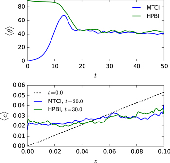
Figure 10. Upper panel: evolution of the average inclination of the magnetic field for the MTCI and the HPBI. Both instabilities seem to drive the average inclination toward 45°. Lower panel: the average along x of c for the MTCI (blue) and the HPBI (green) at the end of the exponential phase of the simulations (t = 30). The initial gradient in c (dashed black line) is diminished by the instabilities.
Download figure:
Standard image High-resolution imageThe helium mass concentration, c, dramatically changes, and the initial gradient is diminished by the instability as time progresses. This is illustrated in the lower panel of Figure 10 for both the MTCI and the HPBI. As explained in the introduction, gradients in composition can introduce biases in key cluster parameters. We are therefore interested in understanding whether such gradients, if initially present, will be robust. The simulations presented here are heavily idealized, among many reasons because the gas is assumed to be initially isothermal and the simulations are local. Nevertheless, these simulations serve as a proof of principle that gradients in composition can indeed be altered by turbulent mixing induced by plasma instabilities. Future work, using realistic gradients for temperature and composition as well as transport coefficients, should allow us to understand whether such mixing can occur on timescales relevant for galaxy clusters.
6. SUMMARY AND DISCUSSION
In this paper we have introduced a modified version of Athena (Stone et al. 2008) for performing kinetic MHD simulations of weakly collisional plasmas with nonuniform composition. We have employed this modified code to perform the first simulations of the MTCI, the HPBI, and the diffusion modes introduced in Pessah & Chakraborty (2013). The set of simulations, aimed at investigating the linear evolution of these instabilities, served as a test for both the modification to Athena and the local linear mode analysis in Pessah & Chakraborty (2013) and Berlok & Pessah (2015).
The simulations of weakly collisional, isothermal atmospheres with a gradient in helium presented in Section 5 showed that the plasma instabilities, feeding off gradients in composition, can induce turbulent mixing of the helium content. This conclusion is valid for compositions that increase in the direction anti-parallel to gravity, regardless of whether the initial magnetic field is parallel or perpendicular to the direction of gravity. In the saturated state, the magnetic field components in the x and z directions have roughly the same average energy, but the energies are a factor of 10 higher for the HPBI than for the MTCI. The kinetic energy components are also roughly in equipartition. In both cases, the instabilities saturate by driving the average magnetic field inclination to roughly 45°. This effect seems to open the possibility of alleviating the core insulation observed in previous homogeneous simulations of the HBI, provided that the global cluster dynamics were to allow for an increase in the mean molecular weight with radius in the inner region, as envisioned by current (one-dimensional, unmagnetized) helium sedimentation models (Peng & Nagai 2009).
The simulations of the nonlinear regime of the MTCI and the HBPI presented in this paper considered an isothermal atmosphere as the equilibrium background. It would be an improvement to use the model of Peng & Nagai (2009) to determine the gradients in both temperature and composition. This would provide insight into the saturation of instabilities in potentially more realistic scenarios where the dynamical evolution is determined by the simultaneous effects of both gradients. Before proceeding with this endeavor, there are, however, a few issues that would be desirable to address, as we detail below.
It was found in Berlok & Pessah (2015) that the HPBI, if present in the inner regions of the ICM model of Peng & Nagai (2009), will have its fastest growth rates at wavelengths that are longer than the scale height of the atmosphere. This conclusion is similar to what was found for the HBI in Kunz (2011). Neither local linear theory nor local simulations will therefore capture the physics of the HPBI in the inner region of the ICM. This implies that both a quasi-global theory and simulations are needed in order to study the influence of the possible gradient in composition on the dynamics of the inner region of the ICM.
Local simulations of the MTI have been shown to underestimate the turbulence (McCourt et al. 2011), and boundary effects can also modify the conclusions from local simulations. The solution to this problem for the MTI has been to sandwich the unstable region between stable layers, thereby isolating it from the boundaries (Parrish & Stone 2005, 2007; Kunz et al. 2012). A similar approach seems reasonable for the MTCI.
Other complications stem from the fact that pressure anisotropies, shown to be important for the evolution of the MTI and HBI (Kunz 2011; Kunz et al. 2012), can give rise to microscale instabilities such as the firehose and mirror instability (Schekochihin & Cowley 2006; Schekochihin et al. 2010). These small-scale instabilities are only excited once the pressure anisotropy grows beyond  . They do not appear in the tests of the linear regime of the MTCI, HPBI, and the diffusion modes presented in Section 4 because we terminate the simulations before the stability criterion is violated. They are not present in the simulations of the nonlinear regime in Section 5 because we take the pressure to be isotropic in these simulations (no Braginskii viscosity). The problem with microscale instabilities is that they are not correctly described by the framework of kinetic MHD (Schekochihin et al. 2005), an issue that will need to be addressed for simulations of the nonlinear evolution of the MTCI and the HPBI when Braginskii viscosity is included (see Kunz et al. 2012 for a discussion of these issues in the context of the MTI and the HBI).
All this being said, our study suggests that, at least in the idealized settings that we considered here, gradients in composition are able to drive turbulent mixing of the composition in weakly collisional, magnetized plasmas. This motivates future work on the generation and sustainment of both temperature and composition gradients in galaxy clusters and their potential influence on the global dynamics of the ICM. We envision that the modified version of Athena that we developed will be a useful asset in this context. In order to model more realistically the physics of the ICM, future improvements could include extending the simulations to three dimensions and adding optically thin cooling in order to study the cooling flow problem. Furthermore, the equations of kinetic MHD, as embodied in Equations (1)–(5), cannot account for the slow sedimentation of helium that is the core feature in the model of Peng & Nagai (2009). An extension of the framework of kinetic MHD to include this effect would allow us to self-consistently include sedimentation in the simulations (Bahcall & Loeb 1990; Berlok & Pessah 2015) and study the effects of the instabilities described in this paper in a dynamic, slowly varying background.
We acknowledge useful discussions with Daisuke Nagai, Matthew Kunz, Prateek Sharma, Ellen Zweibel, and Ian Parrish during the 3rd ICM Theory and Computation Workshop held at the Niels Bohr Institute in 2014. We thank Sagar Chakraborty, Colin McNally, Gareth C. Murphy, and Henrik Latter for valuable discussions and comments. We are grateful to Oliver Gressel for suggesting using the quasi-periodic boundary conditions for testing the linear theory and to Tobias Heinemann for aid in rendering magnetic field lines. We also thank the anonymous referee for a number of useful suggestions that helped improve the manuscript. The research leading to these results has received funding from the European Research Council under the European Union's Seventh Framework Programme (FP/2007–2013) under ERC grant agreement 306614. T.B. also acknowledges support provided by a Lørup Scholar Stipend, and M.E.P. also acknowledges support from the Young Investigator Programme of the Villum Foundation.
APPENDIX
In this appendix, we describe the numerical methods used in this paper. We use the publicly available MHD code Athena, which solves the conservative form of the MHD equations. The algorithms used are described in Gardiner & Stone (2005) and Stone & Gardiner (2009), and the implementation of Athena along with tests is described in detail in Stone et al. (2008). Athena is a finite-volume code, which uses the Godunov method. We use the directionally unsplit corner transport upwind method along with constrained transport (CTU + CT), which is the recommended setting. We furthermore use the anisotropic heat conduction module that was implemented in Athena by Parrish & Stone (2005) using operator splitting.
Appendix A explains the implementation of a spatially varying mean molecular weight, μ, the anisotropic diffusion of helium and tests cases, in Athena. In Appendix B we discuss in detail the boundary conditions used in the simulations.
APPENDIX A: IMPLEMENTATION OF ANISOTROPIC DIFFUSION OF COMPOSITION IN ATHENA
Let us consider the equation describing the evolution of the helium mass concentration,  , given by6

Athena has an option for adding passive scalars, which we use for adding the helium mass concentration. This option turns on an extra equation,

where ρ is the total density and  is the mass concentration of the nth scalar. We only add a single scalar, namely, the helium mass concentration, c. This built-in function takes care of the Lagrangian part of Equation (25). The diffusion term is then solved using a finite-difference scheme and operator splitting.
Anisotropic diffusion of helium is described by the right-hand side of Equation (25), which, when  , reduces to

The composition flux for anisotropic helium diffusion has the same form as the heat flux for anisotropic heat conduction, as seen by comparing Equations (12) and (11), respectively. We can therefore use the same method to calculate the two physically different anisotropic fluxes. The original implementation of anisotropic heat conduction was done by Parrish & Stone (2005) using an asymmetric finite-difference scheme (Sharma & Hammett 2007; van Es et al. 2014).
Nonideal effects are computationally expensive because they are generally described by parabolic operators that cannot be added to the hyperbolic fluxes used in the Godunov scheme. The parabolic operators can be shown to have a very prohibitive time-step constraint (Durran 2010) for heat conduction and concentration diffusion as given by, respectively,


Here  is the heat diffusivity, the parameter b is
  in one, two, and three dimensions, respectively, and
  is the grid size.
The Courant number, C, is defined to be the ratio of the applied time step to the allowed time step. We use C = 0.4 in all our simulations. Because  , the very prohibitive constraints on the time step for the parabolic operators will generally lead to
  . In order to partially circumvent this problem, we use subcycling, taking up to 10 diffusion steps for each MHD step, as suggested in Kunz et al. (2012).
Sharma & Hammett (2007) found that the finite-difference approximation can lead to unphysical behavior with diffusion in the wrong direction. In the context of heat diffusion this problem can lead to negative temperatures and therefore an imaginary sound speed. The same problem arises when considering helium diffusion, and we use van Leer limiters on the derivatives to circumvent it (Sharma & Hammett 2007).
The publicly available version of Athena works with constant viscosity,  , and heat diffusivity,
  . However, these coefficients, as well as the diffusion coefficient D, do in general depend on temperature, density, and composition; see, for instance, the discussion in the appendix of Berlok & Pessah (2015). Accounting for this dependence is not crucial in local simulations, but it becomes essential in global simulations. We have modified Athena to use spatially varying coefficients by using a harmonic average of the coefficients (Sharma & Hammett 2007). This makes the time step computed from Equations (28) and (29) spatially dependent. We therefore calculate the time step at each cell and use the minimum value. This implementation will be useful in future global studies.
A.1. Tests of the Implementation of Anisotropic Diffusion
In order to verify the implementation of anisotropic diffusion of helium, we performed three different test problems with a known analytical solution. These tests were carried out with the MHD solver turned off.
A.1.1. One-dimensional Diffusion
We consider the diffusion of a step function as in Rasera & Chandran (2008) using a one-dimensional grid with 100 cells on the domain ![$x=[0,1]$](https://content.cld.iop.org/journals/0004-637X/824/1/32/revision1/apj523632ieqn178.gif) with D = 1 and run the simulation up to t = 0.0028. The analytical solution to the diffusion of a step function is
with D = 1 and run the simulation up to t = 0.0028. The analytical solution to the diffusion of a step function is

where  and
and  . The "+" sign is used with
  for
for  and the "−" sign is used with
  for
for  . The numerical result matches the analytical solution, as seen in Figure 11, implying that the method works well in one dimension.

Figure 11. Diffusion of a step function. The initial condition is shown with a dashed line. The green crosses correspond to data from the simulation, and the solid blue line is the analytical solution at t = 0.0028.
Download figure:
Standard image High-resolution imageA.1.2. Diffusion of a 2D Gaussian
A more challenging test can be posed by considering the magnetic field to be inclined at an angle, θ, with respect to the grid. We consider an initially isotropic, 2D Gaussian distribution of helium diffusing out along an inclined magnetic field. The analytical solution is7
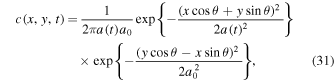
where  and a0 is the initial standard deviation of the Gaussian.
The computational domain is a ![$[-1,1]\times [-1,1]$](https://content.cld.iop.org/journals/0004-637X/824/1/32/revision1/apj523632ieqn186.gif) Cartesian box. We use
Cartesian box. We use  and D = 0.001. The errors at t = 4 are compared to the analytical solution in Figure 12. In the left panel the L2 errors are shown as a function of the magnetic field inclination and resolution. These errors are smallest when
  or
or  , corresponding to the grid and the magnetic field being aligned. In the right panel we show that the solution for
  converges as
  where
where  is the (uniform) grid spacing and m = 1.9 is the order of convergence.
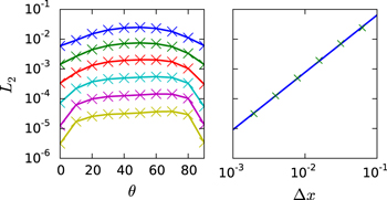
Figure 12. Left: L2 error as a function of magnetic field inclination. Resolutions of N × N with  ,
,  , and 1024 were used with monotonically decreasing L2 at all angles. As expected, the asymmetric finite-difference scheme gives the best result when the magnetic field is aligned with the grid. Right: convergence to the exact solution with decreasing
  for a magnetic field inclined at 40° from the x-axis.
Download figure:
Standard image High-resolution imageA.1.3. Diffusion of a High-concentration Patch in a Circular Magnetic Field
The final and most challenging test that we carry out for anisotropic transport was introduced in Parrish & Stone (2005). We consider a Cartesian box of size ![$[-1,1]\times [-1,1]$](https://content.cld.iop.org/journals/0004-637X/824/1/32/revision1/apj523632ieqn196.gif) with a patch with higher concentration c, specifically8
with a patch with higher concentration c, specifically8
The density is uniform with  , and the magnetic field is circular. In order to ensure
  , the magnetic field was initialized with a vector potential satisfying
  .
.
We considered the value D = 0.01 and run the simulation until t = 200. The overconcentration diffuses out along the magnetic field lines, as observed in Figure 13. We have run this test problem with the same resolutions as Sharma & Hammett (2007) and obtain the exact same values quoted there for the error norms associated with the resolutions 200 × 200 and 400 × 400. For instance, for a resolution of 200 × 200, we obtain  ,
,  , and
, and  at t = 200 as stated in Sharma & Hammett (2007).

Figure 13. The patch with a high concentration of c diffuses out along the circular magnetic field. Snapshots at  , and 200. The color scale is from 10 to 10.2, and the perpendicular diffusion is small. The resolution in this numerical experiment is 400 × 400.
Download figure:
Standard image High-resolution image
It is evident from Figure 13 that, even though only anisotropic diffusion is explicitly turned on, there is still a small amount of numerical, perpendicular diffusion. This is undesired in simulations of instabilities because isotropic diffusion will lower the growth rates or even quench the instabilities. This was investigated by Parrish & Stone (2005) for the MTI, who found that it is, however, insensitive to perpendicular diffusion provided that  . The fact that we find the correct analytical growth rates for all simulations discussed in Section 4 shows that the numerical perpendicular diffusion is not a problem for our present purposes.
APPENDIX B: BOUNDARY CONDITIONS
In the horizontal direction we use the periodic boundary conditions that Athena provides as a standard option. In the vertical direction, boundary conditions that maintain hydrostatic equilibrium are required. In this section we describe the conventional, reflective boundary conditions, as well as the quasi-periodic boundary conditions alluded to in Section 3.2.
B.1. Reflective Boundary Conditions
Our implementation of reflective boundary conditions follows the description in Zingale et al. (2002). Hydrostatic equilibrium requires that Equation (13) is satisfied. This requirement can be approximated by

where a = 1 ( ) at the top (bottom) of the domain. In this notation, i refers to cell i and
  refers to one cell further up (down) when a = 1 (
 ). This equation is then solved for
  using that

along with an assumption on  and
and  . Either one can assume
  and
and  , or one can prescribe the values at the boundaries to be equal to their initial values, i.e.,
  and
and  . In the case where the mean molecular weight μ is not included, Parrish & Stone (2005) refer to these boundary conditions as adiabatic and conductive, respectively. A combination of these two boundary conditions is also possible (i.e., fixing μ and varying T or vice versa). We have implemented all four combinations but will only discuss the conducting boundary conditions (
 and
and  ) in the following, since these are the boundary conditions used in Section 5.
Solving Equations (33) and (34) for  and
and  , we find

and  , where

These relations are used to calculate the density and pressure of the four ghost zones at the top and bottom of the computational domain. At the same time, velocity is reflected symmetrically around z = 0 and  . The magnetic field components are also mirrored. In the case of an initially vertical magnetic field, we let the Bx component change sign, whereas in the case of an initially horizontal magnetic field, we let the Bz component change sign. This forces the field to remain vertical (horizontal) at the boundary in the case of an initially vertical (horizontal) field.
Athena uses the Godunov scheme, which is known not to be optimal at maintaining hydrostatic equilibrium (Zingale et al. 2002). The reason is that the pressure term in the momentum equation is not solved simultaneously with the gravity term. There are ways to modify a Godunov scheme such that this problem is circumvented; see, for instance, Zingale et al. (2002) and Käppeli & Mishra (2014). We use a high numerical resolution and a low Courant number (C = 0.4) in order to maintain hydrostatic equilibrium as well as possible. The minimum amplitude we can use for perturbations in  is, however, limited by the numerical noise caused by the inability of the code to perfectly maintain hydrostatic equilibrium, in agreement with the findings of Parrish et al. (2012b).
B.2. Quasi-periodic Boundary Conditions
A key assumption in standard local linear mode analysis, such as presented in Pessah & Chakraborty (2013) and Berlok & Pessah (2015), is that the perturbations have the spatial dependence  . This assumption is not fulfilled for the reflective boundary conditions, and it is thus impossible to cleanly excite a single eigenmode, the problem being that the boundary conditions excite other modes in an uncontrolled way. We originally realized this problem when we studied the HBI, but it persists in the case of the HPBI and its diffusive variant. The problem is not present for the MTI and the MTCI in the case kz = 0 because the boundaries are periodic in x.
We have developed special boundary conditions that are consistent with the assumptions used in the local mode analysis. One of the key assumptions here is that the perturbed quantities  ,
,  , and
, and  are periodic. In the following, the values outside the computational domain (the ghost zones) are denoted by a subscript g, and the values on the inside are denoted by a subscript i. The subscript "eq" refers to the value of the equilibrium background (as given in Sections 3.1.1 or 3.1.2). The mapping from interior to ghost zones (
 ) is the same as for periodic boundary conditions. Instead of directly mapping the interior values to the ghost zones, we let the ghost zones depend on the change in the interior values with respect to the equilibrium background. The quasi-periodic boundary conditions are then defined as


with the pressure given by  . The equilibrium magnetic field and velocity do not have a gradient, and so their boundary conditions are simply periodic, i.e.,
  and
and  . These are the boundary conditions we used in Section 4.
Footnotes
- 1
- 2
Note that this definition of β differs from the one in Berlok & Pessah (2015) by a factor of 2.
- 3
We consider high-β plasmas and do not include the magnetic pressure in the derivations of the equilibria.
- 4
We note that ky = 0 in all the simulations presented in this paper.
- 5
The boundary conditions on the magnetic field are also slightly different; see Appendix B.
- 6
We do not consider the effects of thermo-diffusion and baro-diffusion, which makes our current model unable to describe the slow sedimentation of helium (Bahcall & Loeb 1990) that can give rise to a composition gradient.
- 7
This result can be derived by solving the one-dimensional diffusion equation for a Gaussian initial distribution followed by a rotation of the coordinate system. The one-dimensional problem is solved by using a Fourier transform in space and a Laplace transform in time.
- 8
This test was constructed for the anisotropic heat conduction. We are using the same initial values (10 and 12) as in the literature, making it easier to compare the results. These values are of course not meaningful values for c, but it still serves as a test of the implementation of anisotropic diffusion. The same considerations apply to the step function test.