


ABSTRACT
We present extensive optical (UBV RI,  , and open CCD) and near-infrared (ZY JH) photometry for the very nearby Type IIP SN 2013ej extending from +1 to +461 days after shock breakout, estimated to be MJD 56496.9 ± 0.3. Substantial time series ultraviolet and optical spectroscopy obtained from +8 to +135 days are also presented. Considering well-observed SNe IIP from the literature, we derive UBV RIJHK bolometric calibrations from UBV RI and unfiltered measurements that potentially reach 2% precision with a B − V color-dependent correction. We observe moderately strong Si ii
  as early as +8 days. The photospheric velocity (
 ) is determined by modeling the spectra in the vicinity of Fe ii
  whenever observed, and interpolating at photometric epochs based on a semianalytic method. This gives
  km s−1 at +50 days. We also observe spectral homogeneity of ultraviolet spectra at +10–12 days for SNe IIP, while variations are evident a week after explosion. Using the expanding photosphere method, from combined analysis of SN 2013ej and SN 2002ap, we estimate the distance to the host galaxy to be
  Mpc, consistent with distance estimates from other methods. Photometric and spectroscopic analysis during the plateau phase, which we estimated to be 94 ± 7 days long, yields an explosion energy of
  erg, a final pre-explosion progenitor mass of 15.2 ± 4.2
  and a radius of 250 ± 70
  . We observe a broken exponential profile beyond +120 days, with a break point at +183 ± 16 days. Measurements beyond this break time yield a 56Ni mass of 0.013 ± 0.001 M
 .
.
Export citation and abstract BibTeX RIS
1. INTRODUCTION
Supernovae (SNe) exhibiting substantial hydrogen in their spectra are classified as Type II (Filippenko 1997). These events are considered to result from the sudden core collapse (CC) of massive stars that still retain substantial hydrogen envelopes. Early-time spectra are basically blue continua with P Cygni lines of hydrogen. SNe II manifest in a variety of subtypes, with SNe IIP yielding distinctive plateaus of bright optical emission lasting roughly 100 days. The plateau phase is believed to arise from a particularly extended hydrogen outer layer that sustains optical emission through recombination as the photosphere recedes and the outer envelope cools over time. After the plateau phase ends, subsequent evolution is powered by radioactive decay. This behavior yields direct measurement of radioactive material produced from the explosion. While some variation is observed in the late-time properties among SNe IIP, variation is more evident in the properties during early times and the photospheric phase, such as rise time, absolute peak magnitude, plateau length and slope (e.g., Anderson et al. 2014). Unlike thermonuclear SNe Ia, which are thought to come mostly from near-Chandrasekhar-mass white dwarf thermonuclear explosions, SNe IIP are believed to arise from massive progenitors (Heger et al. 2003; Utrobin & Chugai 2009) ranging from 8 to 25  . Using pre-SN imaging data, Smartt et al. (2009) obtained a Zero-Age Main Sequence (ZAMS) mass range of 8–17
  for these events. Nevertheless, their characteristics have lent themselves to use as cosmic distance indicators and possible independent probes of dark energy (Hamuy et al. 2001; Hamuy & Pinto 2002; Nugent et al. 2006; Poznanski et al. 2010).
SNe IIP present the opportunity to measure a wealth of physical parameters from the explosion, and the extensive data available for nearby events are crucial to pinning down the mechanisms involved. This, in turn, is important to any use as cosmological probes from the most frequently occuring SN types (e.g., Li et al. 2011).
On 2013 July 25 (UT dates are used throughout this paper), discovery with the 0.76 m Katzman Automatic Imaging Telescope (KAIT) at Lick Observatory of a new SN IIP in M74 was announced (Kim et al. 2013). This made SN 2013ej one of the closest SNe ever discovered. Prediscovery photometry was obtained with the Lulin telescope (Lee et al. 2013) and the ROTSE-IIIb telescope at McDonald Observatory (Dhungana et al. 2013), making this also one of the best-observed young SNe IIP. Follow-up spectroscopy was performed using the Hobby Eberly Telescope (HET), and the Kast spectrograph at Lick Observatory, providing a classification and a redshift. Valenti et al. (2014) performed an analysis of the first month of photometry and spectroscopy, yielding constraints on the object and indicating it to be one of the more slowly evolving SNe IIP at early times. They identified a moderately strong Si ii feature, blueward of Hα in the first month. Pre-explosion images obtained with the Hubble Space Telescope (HST) were analyzed by Fraser et al. (2014), from which they proposed two possible progenitors, with the redder source being the more likely candidate. Using an M-type supergiant bolometric correction, they estimated the mass of the progenitor to be  . More recently, from hydrodynamic simulations, Huang et al. (2015) found the progenitor to be a red supergiant with a derived mass of 12–13
  prior to explosion. We also note that, from an independent data set, Bose et al. (2015a) have favored SN 2013ej to be a Type IIL event, accounting for the observed steep plateau and the systematically high velocity of strong H i lines.
We present an extensive analysis of unfiltered CCD and broadband photometry from the ultraviolet (UV) through the infrared (IR), and a time series of UV and optical spectroscopy, for SN 2013ej. We consider all the measurements relative to 2013 July 23.9 (MJD 56496.9) unless otherwise explicitly stated. Section 2 presents the data, while Section 3 describes the photometric and spectroscopic reductions. Utilizing open-CCD and broadband photometry, we analyze the early-time photometry to derive the time of shock breakout in Section 4. This section also presents bolometric calibration of unfiltered and broadband photometry, as well as a derivation of photometric observables such as color and temperature. Analysis of UV and optical spectroscopic features from +8 to +135 day is discussed in Section 5. In Section 6 we derive the photospheric velocity at photometric epochs, from which we utilize the expanding photosphere method (EPM) to estimate the distance to SN 2013ej. Kinematics of the explosion, properties of the progenitor, Ni mass yield, and other physical properties are derived in Section 7. The discussion and our conclusions are presented in Section 8.
2. OBSERVATIONS
2.1. Photometry
SN 2013ej was discovered by the Lick Observatory Supernova Search (LOSS; Filippenko et al. 2001) on 2013 July 25.45 (Kim et al. 2013), using unfiltered data taken with KAIT. A color combined frame of the SN 2013ej and the host galaxy M74 is shown in Figure 1. The 0.45 m ROTSE-IIIb telescope also observed SN 2013ej in automated sky patrol mode, first on 2013 July 31.36. ROTSE-IIIb is operated with an unfiltered CCD with broad wavelength transmission over the range 3000–10600 Å. Precursor ROTSE images from July 14.42 rule out any emission at a limiting magnitude of 16.8. Careful analysis of additional ROTSE-IIIb observations reveals the earliest detection at July 25.38, about 100 minutes prior to the discovery epoch (Dhungana et al. 2013). Following discovery, we scheduled follow-up observations with the goal of obtaining well-sampled photometry of this bright, nearby SN. Unfortunately, weather conditions were not optimal for the following 5 days for ROTSE-IIIb when the SN was nearing its peak. We then continued observations for 200 days (see Figure 2).

Figure 1. Field around SN 2013ej on a color-combined (BV I) CCD frame taken with the 0.6 m Schmidt telescope at Konkoly Observatory, Piszkesteto, Hungary. Konkoly photometry reference stars in the vicinity of SN 2013ej are shown.
Download figure:
Standard image High-resolution image
Figure 2. Open CCD and multiband photometry of SN 2013ej. KAIT BV RI and unfiltered data points are shown with empty circles, while Konkoly BV RI and ROTSE points are solid circles. Swift photometry is represented with filled square symbols.
Download figure:
Standard image High-resolution imageWe obtained broadband photometry with the 60/90 cm Schmidt telescope of the Konkoly Observatory at Piszkesteto Mountain Station, Hungary, through Bessell BV RI filters. This Konkoly data set spans from +8 to +130 day. Photometric observations were also performed at Baja Observatory, Hungary, with the 50 cm BART telescope equipped with an Apogee-Ultra CCD and Sloan  filters.
Photometry was also obtained with the multi-channel Reionization And Transients InfraRed camera (RATIR; Butler et al. 2012) mounted on the 1.5 m Johnson telescope at the Mexican Observatorio Astronom´ico Nacional on Sierra San Pedro Mártir in Baja California, México (Watson et al. 2012). Typical observations include a series of 80 s exposures in the ri bands and 60 s exposures in the ZY JH bands, with dithering between exposures. Near-IR data from RATIR span from +3 to +125 day.
In addition to the unfiltered data taken in discovery mode, scheduled follow-up Bessell BV RI photometry was obtained with KAIT and the Nickel 1 m telescope located at Lick Observatory. Starting on June 30, a thorough sample of both unfiltered and BV RI measurements was obtained until late in the nebular phase. Unfiltered KAIT data extend to +213 day, while BV RI data span from +7 to +461 day (see Figures 2 and 22).
SN 2013ej was also monitored with the UVOT instrument onboard the NASA Swift space telescope through the uvw2, uvm2, uvw1, u, b, v filters. These frames were collected from the Swift archive.15 Swift data range from +7 to +138 day. The Swift data set has been published by Valenti et al. (2014), Huang et al. (2015), and Bose et al. (2015a). Our reduction of Swift frames is consistent with these works in the u, b, and v filters in the plateau, and until +30 day after the explosion in the uvw2, uvm2, and uvw1 filters. However, we obtain significantly brighter magnitudes than Huang et al. (2015) beyond +30 day in the later three filters. Given the fact that uvw2, and uvw1 filters have extended red tails (e.g., Ergon et al. 2014) and using our photometry, all three of these have a marginal contribution to the total flux after +30 day, we ignore the flux from uvw2, uvm2 and uvw1 bands beyond this epoch (also see Section 4.5).
We also note that the detection of SN 2013ej at its youngest observed phase was announced by Lee et al. (2013) in the BVR bands, on July 24.8, which is 15 hr earlier than the first ROTSE-IIIb detection. A nonphotometric prediscovery detection on images taken on July 24.125 was also reported by C. Feliciano on the Bright Supernovae website.16 No emission on 2013 July 23.54 at V = 16.7 mag was seen by ASAS-SN (Shappee et al. 2013).
2.2. Optical and Ultraviolet Spectra
A total of 17 low-resolution optical spectra of SN 2013ej were obtained using the Marcario Low-Resolution Spectrograph (LRS; Hill et al. 1998) on the 9.2 m Hobby-Eberly Telescope (HET) at McDonald Observatory, the dual-arm Kast spectrograph (Miller & Stone 1993) on the Lick 3 m Shane telescope, and the DEep Imaging Multi-Object Spectrograph (DEIMOS; Faber et al. 2003) on the Keck II 10 m telescope. The Kast and DEIMOS observations were aligned along the parallactic angle to reduce differential light losses (Filippenko 1982). These optical spectra span from +8 to +135 day.
Near-UV spectra of SN 2013ej were taken with UVOT/UGRISM onboard Swift, covering the wavelength range 2000–5000 Å and spanning +8–16 day.
3. DATA REDUCTION
3.1. Photometry
ROTSE data were reduced online using an image-reduction pipeline (Yuan & Akerlof 2008), followed by a DAOPHOT-based point-spread function (PSF) photometry technique (Stetson 1987). Because of significant photometric artifacts and reduced efficiency of image differencing, we performed aperture photometry of SN 2013ej (e.g., Marion et al. 2015). An aperture size of 1 full width at half-maximum intensity (FWHM) of the median PSF on each image was considered, and we chose a background-sky annulus having inner and outer radii of 2 and 4.5 times the FWHM. Additionally, a reference template image was smeared to reflect the PSF at each epoch, and the underlying host-galaxy contribution inside the aperture was subtracted. The typical FWHM of the PSF during the observation timescale was 3''–4''. We calibrated the derived relative flux to the R band from the USNO B1.0 catalog. The instrumental calibration and comparison to other data for analysis are presented in Section 4.
Filtered data from Konkoly were reduced with standard IRAF17
routines to get the SN magnitudes. The instrumental magnitudes were transformed to the standard Johnson–Cousins system via local tertiary standards tied to Landolt (1992) standards on a photometric night (see Table 1 and Figure 1). The g'r'i'z' data from Baja Observatory were standardized using ∼100 stars within the  arcmin2 field of view around the SN, taken from the Sloan Digital Sky Survey (SDSS) Data Release 12 catalog. In order to avoid selecting saturated stars from the SDSS catalog, a magnitude cut
  was applied during the photometric calibration.
Table 1. Tertiary Konkoly BV RI Measurements of the Standard Stars in the Vicinity of SN 2013ej Used for Konkoly Photometrya
| Star | α | δ | B | V | R | I |
|---|---|---|---|---|---|---|
| (J2000) | (J2000) | (mag) | (mag) | (mag) | (mag) | |
| 2MASSb J01365863 + 1547463 (A) | 01:36:58.60 | +15:47:47.32 | 13.19 (0.02) | 12.60 (.01) | 12.32 (0.02) | 11.90 (0.02) |
| 2MASS J01365760 + 1546218 (B) | 01:36:57.56 | +15:46:22.04 | 13.95 (0.02) | 13.16 (.02) | 12.77 (0.02) | 12.30 (0.02) |
| 2MASS J01365154 + 1548473 (C) | 01:36:51.51 | +15:48:48.04 | 14.62 (0.03) | 13.99 (.02) | 13.69 (0.02) | 13.26 (0.02) |
| 2MASS J01364487 + 1549344 (D) | 01:36:44.88 | +15:49:35.88 | 15.74 (0.03) | 14.93 (.02) | 14.59 (0.02) | 14.10 (0.02) |
Notes.
aPhotometric uncertainties are given inside parentheses. bTwo Micron All-Sky Survey.Download table as: ASCIITypeset image
PSF photometry was performed on KAIT and Nickel reduced data (Ganeshalingam et al. 2010) using DAOPHOT. Several nearby stars were chosen from the APASS18 catalog, and the magnitudes were first transformed to the Landolt system19 before calibrating KAIT data. We used APASS R band magnitudes to calibrate the KAIT unfiltered photometry. Image subtraction was not performed for KAIT data, as the object was extremely bright and far from the galaxy core.
For RATIR data reduction, no off-target sky frames were obtained on the optical CCDs, but the small galaxy size and sufficient dithering allowed for a sky frame to be created from a median stack of all the images in each filter. Flat-field frames consist of evening sky exposures. Given the lack of a cold shutter in RATIR's design, IR dark frames are not available. Laboratory testing, however, confirms that the dark current is negligible in both IR detectors (Fox et al. 2012). RATIR data were reduced, coadded, and analyzed using standard CCD and IR processing techniques in IDL and Python, utilizing online astrometry programs SExtractor and SWarp.20 Calibration was performed using field stars with reported fluxes in both 2MASS (Skrutskie et al. 2006) and the SDSS Data Release 9 Catalog (Ahn et al. 2012).
Figure 2 shows the final calibrated SN 2013ej light curves in the ROTSE and KAIT unfiltered bands, the KAIT and Konkoly BV RI bands, and the Swift UVOT bands. Comparison of the data from various sources revealed that they are generally consistent within ±0.1 mag in all optical bands. Figure 3 illustrates g'r'i'z' Baja photometry and riZY JH RATIR photometry. Tables 11–15 provide ROTSE, Konkoly, Baja, KAIT and Nickel, and RATIR photometry, respectively.
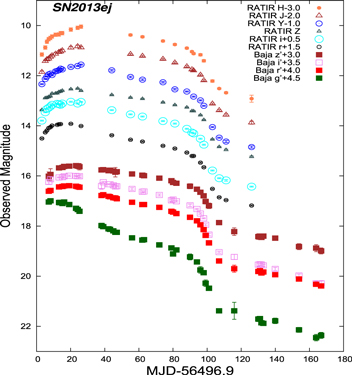
Figure 3. SDSS g'r'i'z' photometry from Baja Observatory, as well as RATIR optical and near-IR photometry, of SN 2013ej.
Download figure:
Standard image High-resolution image3.2. Spectroscopy
All of our optical spectra were reduced using standard techniques (e.g., Silverman et al. 2012). Routine CCD processing and spectrum extraction were completed with IRAF, and the data were extracted with the optimal algorithm of Horne (1986). We obtained the wavelength scale from low-order polynomial fits to calibration-lamp spectra. Small wavelength shifts were then applied to the data after cross-correlating a template sky to the night-sky lines that were extracted with the SN. Using our own IDL routines, we fit spectrophotometric standard-star spectra to the data in order to flux calibrate our spectra and to remove telluric lines (Wade & Horne 1988; Matheson et al. 2000). A log of observed optical spectra is given in Table 2 and plotted in Figure 4. HET spectra are archived on WISEREP21 (Yaron & Gal-Yam 2012), and all of our spectra will be made publicly available from the database.

Figure 4. Time series of optical spectra of SN 2013ej. Phases are in days since explosion (MJD 56496.9). The log of observations is given in Table 2.
Download figure:
Standard image High-resolution imageTable 2. Observing Log of SN 2013ej Optical Spectra
| UT Date | MJD | Epocha (days) | Instrument |
|---|---|---|---|
| 2013 Aug 1.41 | 56505.41 | +8 | HET |
| 2013 Aug 2.46 | 56506.46 | +9 | DEIMOS |
| 2013 Aug 4.38 | 56508.38 | +11 | HET |
| 2013 Aug 4.51 | 56508.51 | +11 | Kast |
| 2013 Aug 8.52 | 56512.52 | +15 | Kast |
| 2013 Aug 12.50 | 56516.50 | +19 | Kast |
| 2013 Aug 30.50 | 56534.50 | +37 | Kast |
| 2013 Sep 6.41 | 56541.41 | +44 | DEIMOS |
| 2013 Sep 10.60 | 56545.60 | +48 | Kast |
| 2013 Oct 1.54 | 56566.54 | +69 | Kast |
| 2013 Oct 5.33 | 56570.33 | +73 | Kast |
| 2013 Oct 8.48 | 56573.48 | +76 | DEIMOS |
| 2013 Oct 10.29 | 56575.29 | +78 | Kast |
| 2013 Oct 26.26 | 56591.26 | +94 | Kast |
| 2013 Nov 2.34 | 56598.34 | +101 | Kast |
| 2013 Nov 8.31 | 56604.31 | +107 | Kast |
| 2013 Nov 28.37 | 56624.37 | +127 | Kast |
| 2013 Dec 6.39 | 56632.39 | +135 | Kast |
Note.
aEpochs are rounded to days since explosion.Download table as: ASCIITypeset image
UV spectra were collected from the Swift archive, and were reduced using the uvotimgrism task in HEAsoft.22 The log of the UGRISM spectral observations is given in Table 3 and the spectra are plotted in Figure 5.
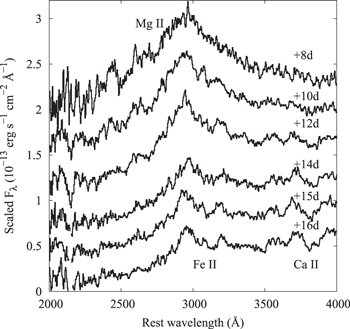
Figure 5. Spectral evolution of SN 2013ej in the UV based on Swift/UGRISM observations. Labels next to each spectrum indicate the days since explosion (MJD 56496.9). Feature identifications are based on Bufano et al. (2009).
Download figure:
Standard image High-resolution imageTable 3. Observing Log of Swift UVOT/UGRISM Spectra
| UT Date | MJD | Epoch | Exposure | S/N |
|---|---|---|---|---|
| (days) | (s) | |||
| 2013 Jul 31.8 | 56504.8 | +8 | 4142 | 30 |
| 2013 Aug 3.1 | 56507.1 | +10 | 4946 | 41 |
| 2013 Aug 4.8 | 56508.8 | +12 | 4896 | 36 |
| 2013 Aug 7.4 | 56511.4 | +14 | 3861 | 25 |
| 2013 Aug 8.2 | 56512.2 | +15 | 4449 | 21 |
| 2013 Aug 9.2 | 56513.2 | +16 | 4449 | 25 |
Download table as: ASCIITypeset image
4. PHOTOMETRIC ANALYSIS
From the lack of narrow Na i D lines from the host galaxy, Valenti et al. (2014) showed that the reddening from M74 in the direction toward SN 2013ej is negligible. No evidence of Na i D lines from the host was seen in spectra of Bose et al. (2015a) and in our own sample. Thus, we do not consider any host extinction. We adopt the Milky Way reddening value of  mag (Schlafly & Finkbeiner 2011) in our data sample. We note that Huang et al. (2015) used
  mag for SN 2013ej based on the V − I color information, while Bose et al. (2015a) adopted
  mag.
mag.
4.1. Early-time Photometry
After explosion, the gravitational waves and neutrinos soon escape while the electromagnetic signal is initially trapped in the envelope. Only when the hydrodynamic front reaches the photosphere, which takes hours to days, is the rise in intensity from the star observed. This epoch indicates the time of first light and marks the beginning of the shock-breakout phase. Precise knowledge of the epoch of shock breakout is crucial to constrain explosion parameters and progenitor properties. It is also instrumental for distance estimates using methods such as EPM (see Section 6).
Several efforts have been carried out to model the shock breakout of the compact progenitor of SN 1987A (e.g., Hoflich 1991; Eastman et al. 1994). Notably, it has been shown that the breakout peak depends upon envelope mass and density structure (Falk & Arnett 1977), so the very early light curve may provide clues on the envelope structure of massive stars. Recently, substantial theoretical studies have been performed with the goal of understanding the shock breakout of SNe II through a variety of processes in several progenitor scenarios (e.g., Nakar & Reém 2010; Svirski & Nakar 2014). Couch et al. (2015) argue that strong aspherical shocks can lead to breakout at different times along the periphery of the star compared to a spherical shock from a spherical star.
To estimate the time of shock breakout for SN 2013ej, we consider several data sets during the first few days. To study the rise behavior, we combine ROTSE and KAIT unfiltered data, calibrated to R magnitudes, with the earliest prediscovery R band detection from Lulin Observatory. Because of the lack of sufficient data points in any of the independent data sets, we calibrate the Lulin R magnitude to the ROTSE magnitude in the following way. We saw a systematic variation of KAIT and Konkoly R band photometry of SN 2013ej. Allowing a similar offset to exist between Lulin R and KAIT or Konkoly R, we calculate the average of differences of KAIT R and Konkoly R magnitudes with ROTSE unfiltered magnitudes and add this as a correction to the Lulin data point to bring it to the ROTSE system. For this, we limit the observations to between +30 and +90 day in the plateau, where they are densely sampled in both sets and the spectral energy distribution (SED) is smooth compared to the rapid evolution during early times (see Section 4.3). Furthermore, we add an additional systematic uncertainty to the Lulin point from the root-mean square (rms) of KAIT R and Konkoly R magnitude differences. We note that the Lulin observation already has an uncertainty higher than 0.2 mag. Any systematic uncertainty that arises from translating the calibration from plateau to early rise time is likely to be smaller than this. Specifically, Butler et al. (2006) found a correction of around of 0.1 mag between KAIT unfiltered and Lulin R band magnitudes for Gamma Ray Burst study. ROTSE unfiltered and KAIT unfiltered data, both of which closely track the R magnitudes to early times, have been independently cross-calibrated to the same unfiltered source for early time studies of both SN Ia and SN IIP (e.g., Quimby et al. 2007; Zheng et al. 2013). On the first night of detection with ROTSE-IIIb, we had better time granularity of about 2 hr between coadds of two sets of images. As the SN was still young (∼1 day after explosion), a significant rise even in only 2 hr is detectable.
A functional form of the SN IIP rise behavior has not been well established. A simple power law, specifically a t2 rise law, has been tested in the context of SNe Ia many times, while recent studies (e.g., Zheng et al. 2013; Marion et al. 2015) have shown departure from t2 rise at very early times. In SNe Ia, the heat loss due to cooling of the ejecta can be thought to be compensated by the radioactive heating, thus maintaining the steady temperature, while in SNe IIP, the adiabatic cooling of the shock-heated envelope is expected to result in a steep drop of temperature. Quimby et al. (2007) fitted the early rise of SN IIP 2006bp with a t2 law at very early times. While t2 may be a valid approximation until a few days after explosion in SNe IIP, it is clearly not valid as long as it seems to hold in SNe Ia.
Keeping this uncertainty in mind, we perform a least-squares fit of the rising light curve of SN 2013ej to a single power law, given by

where A is a constant, t0 is the time of shock breakout, and β is the power-law index. Only data points earlier than +2 day since explosion are considered for fitting, effectively including the first 4 points. None of the fits including data beyond +2 day were consistent with the detection and nondetections. We perform the t0 estimation relative to the Lulin observation point on July 24.8 (MJD 56497.8). As SN 2013ej is a SN IIP with particularly early photometry, we first test the power-law hypothesis by letting β float. This yields  days and
  with
with  (see Figure 6). Keeping
  fixed, we obtain
  days, which corresponds to July 23.9 ± 0.25. The reasonable
  value of 1.47 indicates consistency of the early evolution with the t2 model until ∼2 day after explosion. Deviation of β from 2 might be indicative of asymmetry in the explosion itself and is still an open question. This is an important question for SNe IIP and requires further observation of very early times. For SN 2013ej, while the sparse data do not rule out the the power index of 4.83, the t2 model yields better
  and is consistent with all reported early detections and nondetections. Noting this, we take MJD 56496.9 ± 0.3 as the epoch of shock breakout.
4.2. Unfiltered and Broadband Photometry
SN IIP light curves have a unique signature. After the shock breakout, the hot ejecta are believed to expand violently. The photon diffusion timescale being much longer than the expansion timescale, very little photon energy gets diffused. The ejecta would follow a homologous adiabatic expansion, cooling quickly from the outside. Soon after the ejecta cool to ∼6000 K, hydrogen ions start to recombine, the opacity plummets, and diffusion cooling becomes dominant. This will result in an ionization front that recedes inward as a recombination wave, giving a characteristic, slowly declining, almost linear, plateau phase that lasts for approximately 100 days. This plateau is observed as a result of decreasing opacity because of less scattering due to declining electron density. The photosphere remains contiguous with the receding ionization front. After all the hydrogen recombines, the photosphere recedes into the inner, heavy element core and the light curve transitions to the radioactive tail phase. This tail is expected to decline by the  decay at a rate of 0.98 mag per 100 days if all the gamma-rays and positrons are trapped.
Figure 2 shows the apparent magnitude light curves of SN 2013ej with unfiltered and BV RI broadband observations. Each BV RI set consists of data that starts from around the peak, extends through a characteristic plateau phase lasting about 100 days, and proceeds to the well-observed radioactive tail phase. In the ROTSE light curve, the peak for SN 2013ej occurs at +18 day, where the absolute magnitude reaches −17.5. This peak is consistent with the KAIT unfiltered data, both in phase and magnitude. On both the KAIT and Konkoly BV RI light curves, the peak occurs on +12.5 day in B, +15.5 day in V, +19.5 day in R, and +20 day in I. We do not observe any obvious secondary peak like that seen by Bose et al. (2013) in SN 2012aw at about +50 day in the V band, or an obvious minimum around +42 day in V, which would be indicative of the end of free adiabatic cooling. It is thus more challenging to ascertain the advent of the plateau phase in the photometry. We will estimate the plateau length in Section 7. From their respective peaks, the light curves decline by 0.038, 0.021, 0.016, and 0.012 mag per day in B, V, R, and I (respectively) until +90 day. The Konkoly and KAIT data are consistent in this decline behavior. Our V band slope is steeper compared to the 0.017 mag day−1 given by Bose et al. (2015a). This could possibly be a sampling issue, because their photometry during the plateau is sparsely sampled and the peak is less well constrained.

Figure 6. Early rise behavior of SN 2013ej. Multiple data sets calibrated to ROTSE magnitudes (see text) are shown. Solid lines are power-law fits to data obtained before +2 day since explosion. The triangle point is a nondetection limit on July 23.54 at  mag, shown here for reference. The dashed line indicates the detection on July 24.125 with no photometry available. The inset illustrates the projection of where the emission would be for floating index (green) and fixed index
  (blue).
Download figure:
Standard image High-resolution imageSN 2013ej has one of the steepest plateaus among SNe IIP (see Figure 7 for a comparison with other normal SNe IIP). We note that the B band decline for SN 2012aw was 1.74 mag until +104 day, while the R band showed no change in brightness over the plateau (Bose et al. 2013). Classic SN IIP 1999em also evolved similarly (Leonard et al. 2002), while the more energetic SN 2004et had a faster decline of ∼2.2 mag from the B band peak until +100 day (Bose et al. 2013). The decline rate for SN 2013ej is consistently higher in all bands. Example SN IIL light curves of the recent SN 2013by (Valenti et al. 2015) and the archetype SN 1980K (Barbon et al. 1982) are also shown. The magnitude fall of SN 2013ej in the V band from peak to +50 day is about 0.75 mag. This puts SN 2013ej within the SN IIL category of Faran et al. (2014), where they use a cut of 0.5 mag for a SN IIL event. Valenti et al. (2015) observed a fall of 1.46 ± 0.06 mag in V for SN 2013by, and also pointed out the SN IIP-like behavior in its light-curve drop to the radioactive phase. They show a handful of objects for which the difference of the V band peak and +50 day magnitude is more than 0.5 mag, which would be in the SN IIL class of Faran et al. (2014).
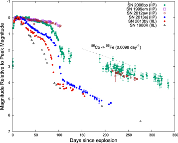
Figure 7. Comparison of some SN IIP and SN IIL light curves in the V band, except SN 2006bp (ROTSE). SN 2013ej has a systematically steeper plateau, with a sharp drop at the end of the plateau. SNe IIL 2013by and 1980K have steep linear evolution after peak, but the drop at the end of the plateau is not as sharp. SN 2013ej also exhibits a steeper tail decline than the events shown here.
Download figure:
Standard image High-resolution imageSN 2013ej, in spite of having such a steep plateau, also exhibits a drop at the end of the plateau that is significantly sharper than the decline in the plateau, which is also a characteristic feature of SNe IIP. A steep plateau for a SN IIP object may also indicate an inefficient thermalization of the ejecta. Additionally, with such a steep plateau, very little nickel yield might be expected. Bersten et al. (2011) showed from hydrodynamic modeling that extensive mixing from 56Ni is required to reproduce flat plateaus. The higher the Ni yield is, the sooner the plateau starts to flatten, and this will also affect the extension of the plateau duration because of radioactive heating.
When the plateau ends at about 100 day after the explosion, the light curve suddenly transitions into the radioactive tail. From the luminosity derived from radiactive decay of synthesized materials, in Section 7 we will estimate the mass of nickel produced. We represent the decline behavior by separate linear fits to the data from +120 to +183 day and from +183 to +461 day. The epoch +120 day was chosen to ensure the late-time decay phase, and +183 was chosen as the break time of the late time behavior (see Section 7.1). Table 4 lists the decay rate along with  per degree of freedom of the respective fits. It is clear that the light-curve decline in the tail is much steeper in all bands and unfiltered photometry before +183 day. Only B band has a slope shallower than
  after +183 day. While SN 2006bp had a tail phase decline of 0.73 ± 0.04 mag per 100 day (Quimby et al. 2007), which is less steep than full trapping of gamma-rays from radioactive decay, SN 2013ej exhibits the opposite behavior.
Table 4. Radioactive Tail Decline Behavior
| Band | +120 to +183 day | +183 to +461 day |
|---|---|---|
| (mag/100 days) | (mag/100 days) | |
| KAIT B | 1.15 ± 0.08 (0.37) | 0.75 ± 0.02 (1.75) |
| KAIT V | 1.46 ± 0.04 (1.01) | 1.10 ± 0.02 (2.69) |
| KAIT R | 1.54 ± 0.04 (2.66) | 1.30 ± 0.01 (3.92) |
| KAIT I | 1.63 ± 0.03 (0.78) | 1.18 ± 0.02 (2.96) |
| KAIT unfiltered | 1.51 ± 0.02 (0.88) | ⋯ |
| ROTSE unfiltered | 1.64 ± 0.07 (1.13) | ⋯ |
| KAIT BV RI | 1.36 ± 0.09 (0.48) | 1.06 ± 0.02 (2.15) |
Note.  are given inside paranthesis.
Download table as: ASCIITypeset image
4.3. Color and SED Evolution
The color evolution of SN 2013ej in the optical exhibits a rapid change in the first 30 days, as shown in Figure 8. This is due to the fact that the U and B fluxes decline rapidly at early phases. While the evolution of B − V is more rapid in the first 30 days, the V − R and V − I colors are smooth and slowly rising. Soon after, when the temperature has fallen to around 6000 K (see Section 4.4), the trends are more alike, and the SED is more uniform. Later, as the light curve approaches the tail, both the V − R and V − I colors show a rapid rise, as an effect from a greater decline of flux in V relative to the I band. The transition from plateau to the tail is evident in both optical and near-IR colors.
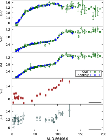
Figure 8. Optical and near-IR color evolution of SN 2013ej. Here, the J − H and Y − Z colors from RATIR are shown in the Vega system for consistency.
Download figure:
Standard image High-resolution imageIn Figure 9, the evolution of the SED ( ) is shown, together with some of the contemporaneous UV and optical spectra (see Section 5). This observed SED evolution is in agreement with the general characteristics of SNe IIP: a strong decline of the UV flux accompanied by a monotonic decrease of the continuum slope in the optical during the plateau phase, in accord with the continuously reddening optical colors seen in Figure 8.

Figure 9. Evolution of the spectral energy distribution (SED) of SN 2013ej. Fluxes from broadband photometry from the UV, optical, and near-IR are plotted with filled circles, and the horizontal bars represent the FWHM of each filter. Phases are coded by colors and indicated in the legends. The optical and UV spectra at certain epochs (where available) are also overplotted for comparison. Dereddening with  mag has been applied.
Download figure:
Standard image High-resolution image4.4. Photospheric Temperature
We determine the temporal evolution of the photospheric temperature by fitting the KAIT and Konkoly BV I fluxes (R fluxes are omitted to avoid contamination from the strong  feature) to a Planck function at each epoch until ∼ +100 day. Beyond this, the light curve enters the radioactive phase, and the energy mostly comes out in strong nebular lines. The BV I set covers the wavelength range 3935–8750 Å. No UV flux is considered, as this would heavily bias the blackbody fits because of the many metallic blends occurring at shorter wavelengths. The temperature drops from 12,500 K at +8 day to 6400 K at +24 day, and it declines very slowly to 4000 K at +100 day as shown in Figure 10. An independent estimate of the temperature by Valenti et al. (2014) is also shown, and it exhibits reasonable agreement with our result. The rapid temperature drop in the first few weeks encapsulates quick adiabatic cooling, while later in the plateau phase the smooth slow decline signifies the cooling from photon energy diffusion during recombination at nearly constant temperature dictated by atomic physics.

Figure 10. Evolution of the photospheric temperature using the KAIT (green points) and Konkoly (blue points) BV I data sets. Temperature estimates from Valenti et al. (2014) are shown with red points.
Download figure:
Standard image High-resolution image4.5. Bolometry
Bolometric photometry permits determination of several explosion parameters, including the direct estimate of the amount of Ni synthesized during the explosion. UV flux in SNe Ia and SNe Ib/c is a small fraction of the total flux, since the high-energy photons are nearly entirely absorbed by transition lines of ionized heavy elements. In SNe II, however, the UV flux dominates at early times. Bright UV and X-ray emission flashes are expected as the shock breaks out, followed by a post-break UV plateau lasting a few days. The spectral index evolves rapidly in the first few weeks, with a large portion of the flux yield in UV. Later evolution transitions to dominant emission in the R, I, and near-IR bands. Without data in all wavebands, it is generally impossible to obtain an exact bolometric flux. The availability of extensive sets of data spanning from UV to IR wavelengths for SN 2013ej gives an ideal opportunity to obtain the most accurate estimate of the bolometric flux for SN IIP. Additionally, this helps to derive bolometric calibration relations for a broadband sample limited in wavelength and unfiltered sets such as from ROTSE or KAIT. We adopt the distance to the SN to be  Mpc (see Section 6) to estimate the integrated luminosity. Pseudo-bolometric and bolometric light curves of SN 2013ej are shown in the top panel of Figure 11. To estimate the bolometric flux in the late time when we do not have UV and NIR observations, we multiply the late time BV RI flux by a scale factor, which we derive by dividing the bolometric flux by the BV RI flux between +120 and +137 day. We also note that the flux from uvw2, uvm2, and uvw1 bands contribute a total of 1% or less to the bolometric flux beyond +30 day according to our reduction (see Figure 11). Photometry by Huang et al. (2015) would contribute much less. Given the marginal contribution from these three bands after +30 day and potential complication of red leaks for uvw2 and uvw1 (e.g., Ergon et al. 2014), these three filters were omitted beyond +30 day in the bolometric flux calculation.

Figure 11. Top panel: integrated BV RI, UBV RI, UBV RIJHK, and bolometric light curves of SN 2013ej. UBV RI and UBV RIJHK shown here are derived using Swift u, KAIT BV RI, RATIR JH, and estimated flux from the K band. The bolometric light curve includes an additional contribution from UV flux below ∼3200 Å before +30 day. Beyond +30 day, UBV RIJHK closely resembles the bolometric light curve in the plateau. Bottom Panel: UV, optical, and near-IR fractional flux. The UV covers flux below the U band, the near-IR (NIR) covers flux above the I band, while optical covers in between (UBV RI). The UV fraction is shown curtailed at the calculated end of plateau, because of the marginal contribution and possible contamination from red tails (see the text).
Download figure:
Standard image High-resolution imageAs a first step, from the fact that the open CCD transmission is broad, we establish a calibration relation for the ROTSE and KAIT unfiltered flux with integrated BV RI flux as follows. Both BV RI data sets are converted to absolute flux using the relations given by Bessell et al. (1998) corresponding to an A0 star (see Table A4 of their paper). The value of  shows a direct relation with the B − V color. A linear fit of
  versus B − V is shown in the top panel of Figure 12. From the rms of the residuals, we obtain a calibration precision of better than 5%, while about 8% precision is obtained from the residual without accounting for the B − V dependence. A similar analysis for KAIT unfiltered and KAIT BV RI data sets yields 4% and 6% precision, respectively, as shown in the bottom panel of Figure 12. A summary of the fits is given in Table 5.

Figure 12. Top panel: pseudo-bolometric BV RI calibration of SN 2013ej from ROTSE unfiltered photometry compared to Konkoly BV RI photometry. Residual from a B − V color-dependent correction (histogram in blue) shows less than 5% uncertainty. The histogram shown on the left (green) is obtained from the residuals by comparing the two fluxes without any color correction. Bottom panel: same as in top panel, but for KAIT unfiltered to KAIT BV RI calibration. We obtain 6% residuals by direct comparison and 4% residuals when applying a B − V dependence. Fit equations for B − V dependence are given in Table 5.
Download figure:
Standard image High-resolution imageTable 5. B − V Dependent Pseudo-Bolometric BV RI and UBV RI Calibration of ROTSE and KAIT Unfiltered Data
| Calibration | Intercept | Slope |

|
|---|---|---|---|
| ROTSE Unf. | |||
| – Konkoly BV RI |

|

|
0.54 |
| KAIT Unf. | |||
| – KAIT BV RI |

|

|
1.58 |
| ROTSE Unf. | |||
| – UBV RI | 0.299 ± 0.009 | 0.161 ± 0.007 | 1.05 |
| KAIT Unf. | |||
| – UBV RI | 0.363 ± 0.006 | 0.112 ± 0.006 | 2.71 |
Download table as: ASCIITypeset image
In the second step, since ROTSE and KAIT unfiltered are also sensitive to the near-UV, we look at the behavior by integrating UV data from Swift. As pseudo-bolometric flux based on Johnson–Cousins UBV RI filters is commonly derived, we first calibrate Swift u to the Johnson–Cousins U band following Poole et al. (2008) and integrate with the BV RI data set. We limit the integration to the wavelength range 3285–8750 Å, where we have extended the lower and upper bounds by the half width at half-maximum intensity (HWHM) in the U and I bands. As before, from observations of the evolution of  , the rms of the residuals after subtracting the mean reveals 13% precision. Calibration with B − V dependence improves the precision to 6% as shown in Figure 13, where a
  of 1.05 is obtained for the fit. Analogously, KAIT unfiltered to UBV RI (using
  and KAIT BV RI) yields about 5% precision after a color-dependent correction, but with larger
  .
.
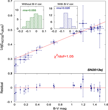
Figure 13. Pseudo-bolometric UBV RI calibration of SN 2013ej from the ROTSE luminosity. The B − V color-dependent correction (histogram in blue) improves the measurement by about a factor of 2 compared to direct comparison (histogram in green).
Download figure:
Standard image High-resolution imageIt is very unusual to obtain a consistently complete set of data for a single object in all bands and still have minimal systematic effects. Various calibration and correction methods have been developed to better estimate the bolometric flux, but all are limited in one way or another. Here we revisit this problem based on the most extensive sets of data from the literature. The calibration sample is provided in Table 6. This set includes extensive photometry from the UV to the IR. To avoid any confusion, we dub the values obtained by integrating fluxes from data as "UBV RIJHK," while we label an equivalent flux derived from our calibration as "UtoK." The same convention also holds in other cases. By "bolometric" flux, we mean integration from  at blue end to H band in the red end, added with contribution from K band as estimated below. We note that the IR flux past K band will be significant as the SN cools over time. We have not accounted for any correction from beyond K band in this procedure.
Table 6. SN IIP Bolometric Calibration Sample Based on Well-sampled Photometry From U Through K
| Object | Host | Distance (Mpc) | Total  (mag) (mag) |
V Plateau Slope (mag/100 days) | Feature | References |
|---|---|---|---|---|---|---|
| SN 1999em | NGC 1637 |

|
0.10 | 0.31 ± 0.05 | Normal | 1, 2, 3, 4 |
| SN 2004et | NGC 6946 |

|
0.41 | 0.72 ± 0.03 | Over Luminous | 5, 6 |
| SN 2005cs | M51 |

|
0.05 | −0.10 ± 0.05 | Subluminous | 7, 8 |
| SN 2013ej | M74 |

|
0.06 | 1.95 ± 0.06 | Normal | This paper |
References. (1) Elmhamdi et al. (2003), (2) Leonard et al. (2002), (3) Krisciunas et al. (2009), (4) Leonard et al. (2003), (5) Sahu et al. (2006), (6) Maguire et al. (2010), (7) Pastorello et al. (2009), (8) Vinkó et al. (2012).
Download table as: ASCIITypeset image
The light curves shown in the top panel of Figure 11 are derived by integrating data in the UBV RIJHK bands, the wavelength range 3285–23850 Å. To obtain the UBV RIJHK flux of SN 2013ej, we integrate the observed flux in the u band from Swift (after calibrating to Bessell U), BV RI from the Konkoly or KAIT data, and near-IR JH data from RATIR, where they are linearly extrapolated in the tail phase. We add an additional contribution from the K band by estimating the average fractional flux in K with respect to the UBV RIJH flux using the calibration sample given in Table 6. We find that the K band contributes ∼2% at +10 day, rising to 5%–6% at +80 day Huang et al. (2015). have published K band data but their data is rather sparse. Comparing their K band measurement with our estimated flux at matching epochs yielded an offset of less than 1% of the total bolometric flux in the plateau while they both agreed in the tail.
From Figure 11, it is clear that the pseudo-bolometric UBV RI flux is significantly lower compared to the bolometric flux, and the difference monotonically grows over time as the source cools. The bolometric luminosity declines very fast, by 0.4 dex in the first 30 days, and relatively slower by another 0.4 dex in the next 50 days. The UBV RIJHK luminosity is significantly different from the bolometric luminosity only before about +20 day; otherwise, UBV RIJHK closely resembles the bolometric flux. The bottom panel of Figure 11 shows the fractional contribution from each of the UV, optical, and near-IR regions to the bolometric flux. The UV portion of the total flux drops from about 38% at +8 day to below 10% by +22 day. After this, the optical contribution drops very slowly and remains above 60% until the end of the plateau, dropping slightly during the tail phase. The near- IR flux contributes about 40% during the plateau phase, and remains almost constant in the tail.
The log of the ratio of UBV RIJHK luminosity to UBV RI luminosity in the calibration sample (Table 6) shows a tight correlation with B − V color. We fit  versus B − V color with a straight line using three of the four objects in this sample (Figure 14). SN 2004et is an energetic, atypical SN IIP with largely uncertain
  it is clearly an outlier, so we do not include it in the final fit given by Equation (2) below:

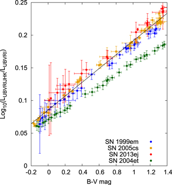
Figure 14. Linear behavior of the log of the ratio of flux with B − V. A tight correlation of  with B − V is seen for SNe 1999em, 2005cs, and 2013ej. The fit has
  . The atypical SN IIP 2004et is shown and not included in the fit. The derived fit is given by Equation (2).
Download figure:
Standard image High-resolution imageThe ratios of the UBV RIJHK and calibrated UtoK luminosities are shown in Figure 15, while the UBV RIJHK light curves are overlaid by calibrated UtoK light curves using Equation (2) in Figure 16. We can now combine the two-fold calibration: (1) ROTSE to UBV RI using the fit shown in Figure 13 (fit parameters are given in Table 5), which gives UtoI, and (2) UtoI obtained in the first step (equivalent to UBV RI) to UtoK using Equation (2). This yields the luminosity of SNe IIP that have B − V and unfiltered photometry. The relative uncertainty from this procedure is about 6% or less. We perform the same analysis for KAIT unfiltered photometry. Figure 17 shows the final calibrated UtoK light curves from ROTSE and KAIT unfiltered photometry for SN 2013ej. Lower panels show the  uncertainty from the calibration. Although the calibration was established by limiting to data before +102 day, it appears to provide reasonable estimates for the bolometric luminosity even during the early nebular phase (see Figure 17).
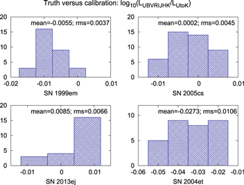
Figure 15. Histograms obtained after subtracting  from
from  . The mean and the rms of the difference confirm 1%–2% precision for SN 2013ej, SN 1999em, and SN 2005cs. Applying the same calibration to SN 2004et (not included in the fit) yields ∼6% precision. Note that the values given in the figures are in
  .
.
Download figure:
Standard image High-resolution image
Figure 16. Comparison of calibrated luminosity with measured luminosity. Solid lines represent UtoK light curves while empty and solid circles represent UBV RI and UBV RIJHK light curves. While 1%–2% precision in the calibration is obtained for SN 2013ej, SN 2005cs, and SN 1999em, the outlier SN 2004et is also calibrated with about 6% precision.
Download figure:
Standard image High-resolution image
Figure 17. UtoK luminosity obtained from calibrating broadband and unfiltered photometry from KAIT, Konkoly, and ROTSE data for SN 2013ej. Data points UBV RIJHK in the top panel are integrated U from Swift, KAIT BV RI, RATIR JH, and an estimated K flux (see text). Shaded regions in the residual plots indicate  uncertainty from the rms of the residuals. For KAIT data, we have added systematic uncertainty based on the differences of KAIT UBV RIJHK and UtoK values derived from UBV RI luminosity using Equation (2), which is derived using Konkoly data. The highest offset at very early times is a result of the high UV contribution to the total flux.
Download figure:
Standard image High-resolution image5. SPECTROSCOPY
5.1. Key Spectral Features
We present 17 optical spectra of SN 2013ej from the HET, Kast, and DEIMOS spectrographs in Figure 4. All of the spectra are corrected for the recession of the host galaxy using z = 0.002192 (NED/IPAC Extragalactic Database23
). This is consistent with that determined by the Supernova Identification software (SNID)24
(Blondin & Tonry 2007) with a fitted redshift of 0.002. Early-time spectra at +8, +9, and +11 day are primarily blue continuum, with a few P Cygni profiles of neutral H Balmer lines and He i lines. The opacity for all other ions is too low to be conspicuously observed as spectral features at these early phases. H i lines (Hα  , Hβ
, Hβ  , and Hγ
  ) are very broad at early times. The strength of emission component of H i lines decreases with time. At +11 day, O i
  is glimpsed. A week later at +19 day, several strong absorption signatures of SNe II appear.
Interestingly, the absorption line to the blue of Hα is unusually strong. This feature, which we identify as Si ii  (see Section 5.3), subsequently becomes stronger until +19 day in our sample. It appears as a small absorption notch at +44 day and disappears by +48 day. Valenti et al. (2014) showed this feature to get stronger than Hα until +21 day in their data set, and to become weaker than Hα by +23 day. The Si ii identification was also favored by Valenti et al. (2014), Bose et al. (2015a), and Huang et al. (2015). Si ii has seemed to occur much later in other SNe IIP. While this strong early appearance of Si ii has not been observed previously, it may have been marginally detected at +10 day and +12 day and was not observed after +25 day in SN 2006bp (Quimby et al. 2007). Si ii is comparatively much stronger than in SN 2006bp at similar epochs. For SN 2006bp, the Si ii velocity profile evolves faster than that of Hα before +25 day, whereas for SN 2013ej, it is more smooth and evolves more slowly than the Hα velocity. All these factors make SN 2013ej exhibit unusual and strong early Si ii.
As the ejecta expand, the subsequent spectral evolution of SN 2013ej shows typical SN IIP singly ionized lines of Ca ii, Fe ii, Ti ii, Sc ii, and Ba ii. The He i λ5876 line gradually gets weaker until +15 day and is not seen at +19 day. This is evidence of the temperature decreasing below the critical temperature of excitation. More iron-group elements start to appear, corresponding to the commencement of the plateau phase where the photosphere penetrates deeper into the envelope. The same disappearance of He i at around +16 day was also seen in SN 1999em (Leonard et al. 2002) and recently in SN 2012aw (Bose et al. 2013). The Na i D lines are considerably stronger than the lines of other neutral elements, presumably coming from non-LTE effects (Hatano et al. 1999). The Na i D feature is observed after +19 day and is probably blended with He i at +15 day. We do not observe any narrow lines of Na i. No obvious evidence of high-velocity features (HVFs) is seen in our spectra. These observations may indicate negligible interaction of the ejecta with the circumstellar material (CSM). After +19 day, the Ca ii near-IR triplet can be dissociated to at least a doublet at 8520 Å and a singlet at 8662 Å; however, the profile is well blended before +15 day, and we adopt this as a single Ca ii near-IR profile to determine the change in ion velocity with time.
5.2. Spectral Homogeneity in the UV
SNe IIP are known to exhibit a remarkable homogeneity in their UV spectra, as first pointed out by Gal-Yam et al. (2008). They found that the early-phase UV spectra (2000–3000 Å) of SNe 1999em, 2005ay, and 2005cs are very similar, both in the shape of the continuum as well as in the visible spectral features. In comparison, Ben-Ami et al. (2015) recently pointed out that SNe IIb, which are thought to have thinner H-rich envelopes than regular SNe IIP, display relatively strong diversity in their UV spectra.
The paucity of well-observed SNe IIP having early-time UV spectra impedes an in-depth study of this homogeneity verses diversity issue at present. It is therefore important to increase the size of the early-time UV sample. SN 2013ej is a valuable addition to this sample because of its relative proximity, which enabled Swift to obtain near-UV spectra with its UVOT/UGRISM instrument (see Figure 5). Figure 18 compares the +8 day and the +11 day spectra to those of other SNe II taken at similar phases. All of these spectra are corrected for interstellar extinction and scaled to match the fluxes in the region 2500–3000 Å.

Figure 18. Evidence of spectral homogeneity of SNe IIP in the UV at early times. Top panel: SN 2013ej UV spectrum compared with the atypical SN 1987A, which shows a sharp UV cutoff, while the excess flux of SN 2005cs below 2500 Å is suspected to be coming from a different source. Bottom panel: homogeneous SN IIP UV sample at ∼12 day. Also shown for comparison is a SN IIb spectrum, which is clearly distinct from the rest.
Download figure:
Standard image High-resolution imageFigure 18 reveals that SN 2013ej nicely fits into the framework of the UV spectral homogeneity of SNe IIP, at least around 10–12 days after explosion. We find that the similarity is not evident for spectra taken at ∼1 week after explosion (Figure 18, top panel) in our sample. Both SN 1987A and SN 2005cs showed some differences with respect to the spectrum of SN 2013ej at this phase, although the rise of the UV flux in the SN 2005cs spectrum below 2500 Å may not be real. Close inspection of the UVOT/UGRISM frames revealed that this spectrum was contaminated by emission from the zeroth order of a nearby source. Moreover, SN 1987A, which shows a sharp cutoff in the UV flux below 3000 Å, was not a typical SN IIP, as it had a blue supergiant progenitor. Nevertheless, the spectra taken around 11 ± 1 days after explosion confirms the observed similarity nicely (Figure 18, bottom panel). Figure 18 also illustrates a SN IIb UV spectrum at a similar epoch; it differs significantly from the SN IIP sample.
5.3. Line Identification and Spectrum Modeling
Line identifications of most of the features in Section 5.1 were first driven by the study of Hatano et al. (1999) on ion signatures of SN spectra. Additional study and confirmation was performed by Syn++ (Thomas et al. 2011) modeling of a few of the optical spectra as shown in Figure 19. While the synthetic modeling produces most of the ionic signatures, the most obvious Hα profile is not reproduced. This reflects the limitation of a purely scattering code: the emission is underestimated because it does not account for the emission due to recombination cascades. For Hα, there may also be a significant effect from non-thermodynamical equilibrium (NLTE) and time varying effects. The absorption notch blueward of the Hα line in the +11 day and +19 day spectra is fitted with the Si ii line, and we have obtained the fit as shown in Figure 19. One could argue that this feature is an HVF of Hα, but then we would expect to also see HVFs of other Balmer lines. Taking an HVF input with such a high velocity, we were unable to reproduce a decent overall fit. Because of the lack of an HVF for other Balmer lines and no HVFs seen in the near-IR spectra, as reported at similar epochs by Valenti et al. (2014), the HVF hypothesis is disfavored. Clearly, the SiII identification hypothesis will be settled with higher confidence only from more realistic modeling. While Bose et al. (2015a) also identified the blueward notch as a Si ii feature, they have incorporated HVFs for H i lines, albeit blended with the photospheric component, accounting for the broad Balmer lines beyond +42 day in their sample. After +15 day, lines of intermediate-mass elements and iron-group elements start to appear. The s-process products Ba ii and Sc ii are also seen from +19 day until the last spectra in the plateau at +94 day.
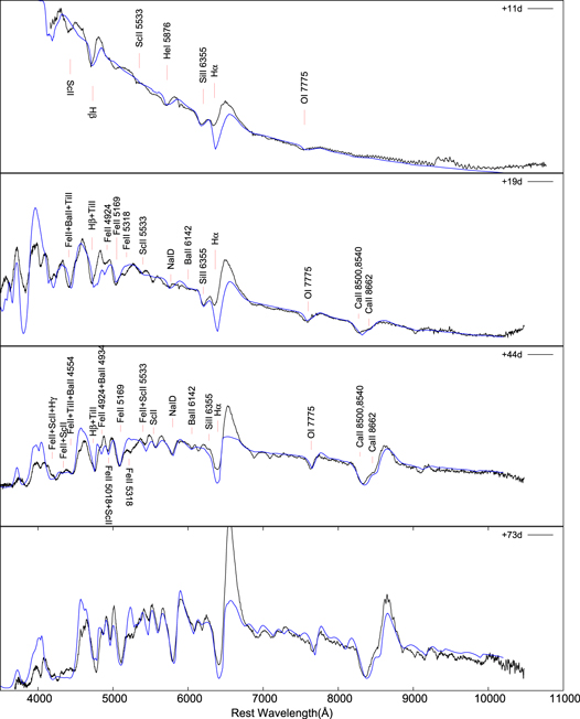
Figure 19. Example Syn++ fits of SN 2013ej spectra are shown in blue while data are in black. The fits mostly reproduce the observed features. The inability to accurately reproduce the H i line profile is perhaps a limitation of the model being purely scattering based and not accounting for the emission from recombination cascades and the NLTE effects. SN 2013ej exhibits most previously identified SN IIP spectral features.
Download figure:
Standard image High-resolution image5.4. Velocity Evolution
While the average ejecta velocity is a direct tracer of kinematic properties, the photospheric velocity not only provides compositional clues but also traces the size of the photosphere, thereby aiding distance measurements (e.g., EPM). The photospheric velocities at early spectral epochs are estimated by fitting the He i  feature. After +19 day, the Fe ii
  line is most indicative of the photospheric velocity, since the minimum of the absorption profile tends to form near the photosphere (Branch et al. 2003).
The velocity evolution of some of the strongest ions is presented in Figure 20. Each line absorption feature is fitted by a Gaussian profile, and the minimum is converted to velocity using the relativistic Doppler equation. The Hα line is decelerating more slowly than Hβ and other metallic ions as expected, but the H i lines show a flat velocity profile, which was also pointed out by Bose et al. (2015a). Poznanski et al. (2010) demonstrated a correlation of velocity of the Fe ii  line (
 ) with that of the
  line (
 ) using 28 optical spectra of 13 SNe IIP covering 5–40 days after explosion. Takáts & Vinkó (2012) have extended the validity of this relation to phases beyond 40 days. We have examined this behavior by taking four optical spectra of SN 2013ej from 15–48 days after explosion. Analysis of Fe ii is not justified before +15 day in our sample. We find that the velocities from SN 2013ej spectra are consistent with this correlation, as can be seen in the right panel of Figure 20. We obtain a linear relation of
  for SN 2013ej, in agreement with
  as obtained by Poznanski et al. (2010).

Figure 20. Left panel: SN 2013ej velocity evolution of strong ions. Empty black circles are the photospheric velocity derived from Syn++ fits. The dashed line is a fit to the photospheric velocity using the method of Vinkó et al. (2012; see the text). Right panel: demonstration of correlation of  with
with  , as suggested by Poznanski et al. (2010). The shaded regions indicate the
  region of the correlation: gray, Poznanski et al. (2010); navy, SN 2013ej (this paper).
Download figure:
Standard image High-resolution imageIn order to refine the photospheric velocity using more than one feature, we first approximate the velocity by estimating from the absorption minimum of the He i  line for the two earliest spectra and the Fe ii
  line for the later spectra. We then performed synthetic spectral modeling with Syn++ and extracted photospheric velocities from the model. Velocities obtained from the fits are given in Table 7.
Table 7. Photospheric Velocities of SN 2013ej Determined by Syn++ Fitting
| MJD | Phase |

|
Uncertainty |
|---|---|---|---|
| (days) | (km s−1) | (km s−1) | |
| 56505.5 | +8 | 10200 | 1000 |
| 56506.5 | +9 | 9700 | 1000 |
| 56508.5 | +11 | 8800 | 800 |
| 56516.5 | +19 | 7660 | 600 |
| 56541.5 | +44 | 4700 | 500 |
| 56545.5 | +48 | 4900 | 400 |
| 56566.5 | +69 | 3200 | 400 |
| 56570.5 | +73 | 3740 | 500 |
Note. Phases are rounded to the nearest day since explosion.
Download table as: ASCIITypeset image
6. DISTANCE DETERMINATION
Recently, the distance to the SN 2013ej host, M74, was subjected to a number of measurements, from the value of  Mpc (Sharina et al. 1996; Vinkó et al. 2004; Van Dyk et al. 2006) to
  Mpc (Zasov & Bizyaev 1996; Olivares et al. 2010); see Table 9 for a summary. Here we revisit this issue by inferring the distance to SN 2013ej via EPM. Modern versions of EPM have been applied for various samples of SNe IIP (Hamuy et al. 2001; Leonard et al. 2002; Dessart et al. 2008; Jones et al. 2009; Vinkó et al. 2012; Bose & Kumar 2014; Takáts et al. 2014). We present the application of the version presented by Vinkó et al. (2012) by combining the data from two SNe that occurred in the same host galaxy, claiming the uncertainties of EPM can be reduced and the reliability of the derived distance improved. Thus, we take the advantage of having the necessary data for both SN 2013ej (this paper) and SN 2002ap (Vinkó et al. 2004), although the latter object is a broad-lined SN Ic for which the application of EPM may not be fully justified. Despite the complications arising in modeling the atmospheres of such stripped-envelope (SE) CC SNe, we show below that the combination of the two data sets results in surprisingly consistent results, and the inferred distance is in very good agreement with recently published independent estimates.
Following the procedure described by Vinkó et al. (2012), the basic equation for EPM is

where t is the time, D is the distance, θ is the angular radius of the photosphere,  is the velocity of the photosphere at t, and t0 is the moment of shock breakout. We estimate θ from the bolometric light curve by using

where  is the dilution factor describing the alteration of the pure blackbody flux in a scattering-dominated SN atmosphere as a function of temperature (Eastman et al. 1996; Dessart & Hillier 2005) and
  is the apparent bolometric flux. For SN 2013ej, we used the dilution factors determined by Dessart & Hillier (2005), which are valid for H-rich SNe IIP, but not for the H-free SE SN 2002ap. Since the atmospheres of such SE SNe are much less known, we set
  as a first approximation. Note that the usage of
  worked surprisingly well when calculating the distance to the Type IIb SN 2011dh (Vinkó et al. 2012). Since the ejecta of the Type Ic SN 2002ap contained practically no H, unlike the Type IIb SN 2011dh, the dilution of the blackbody flux due to Thompson scattering on free electrons might be even less strong than in the case of Type II SNe 2013ej or 2011dh. Thus, setting
  may be a physically realistic approximation for SN 2002ap, although its full justification would involve the computation of an NLTE model atmosphere for SN 2002ap which is beyond the scope of this paper. Nevertheless, we estimate the probable amount of the systematic error of the distance introduced by the assumption of
  below.
The estimates of θ were based on the bolometric light curve of SN 2013ej, as described in Section 4.5. Moreover, we applied the  fluxes of SN 2002ap similarly, after combining the optical light curves from Foley et al. (2003), Pandey et al. (2003), and Vinkó et al. (2004) with the near-IR measurements by Yoshii et al. (2003). In the latter case, the UV contribution was estimated by assuming zero flux at 3000 Å and a simple linear SED between 3000 Å and the U band. This approximation was justified by the shape of the spectra of SN 2002ap as they declined below 4500 Å toward the blue (e.g., Vinkó et al. 2004).
The application of Equations (3) and (4) requires  and
and  values at several epochs, typically during the first 30–50 days after explosion. These can also be estimated directly from the observations. In case of SNe Ic like SN 2002ap, the applicability of EPM is limited to no longer than a few weeks.
For SN 2013ej, values of  were obtained in Section 4.4. For SN 2002ap, we applied the reddening value of
  mag (Vinkó et al. 2004) and the relation

based on the SN Ic-BL models by Mazzali et al. (2000).
In order to increase the sampling of the velocity curve of SN 2013ej, we fit the velocity curve for SNe IIP derived by Takáts & Vinkó (2012) to the velocities obtained in Table 7. This method involves velocity modeling as a power-law expansion of phase, given a model velocity at some epoch. This model velocity is generally derived from synthetic modeling of the observed spectra or by direct measurement from the absorption profile of lines like Fe ii  . See Takáts & Vinkó (2012) for a more detailed discussion of this kind of velocity measurement in SN IIP atmospheres. The result of this fitting was applied in the procedure of EPM.
For SN 2002ap, we adopted the velocities based on the Si ii  feature as given by Vinkó et al. (2004).
The derived quantities needed for EPM are shown in Table 8. The moments of the explosion were set to be t0 = MJD 56496.9 (2013 July 23.9 UT), as derived in Section 4.1) and t0 = MJD 52302.0 (2002 January 28.0 UT) for SNe 2013ej and 2002ap, respectively.
Table 8. Physical Quantities Derived for EPM
| Time | θ |

|
Uncertainty |
|---|---|---|---|
| (days) | (108 km Mpc−1) | (day Mpc−1) | (day Mpc−1) |
| SN 2013ej | |||
| 8.60 | 9.44 | 1.08 | 0.12 |
| 10.60 | 10.10 | 1.24 | 0.12 |
| 13.60 | 11.45 | 1.52 | 0.17 |
| 14.60 | 12.78 | 1.74 | 0.19 |
| 15.60 | 12.98 | 1.81 | 0.20 |
| 16.60 | 13.30 | 1.90 | 0.20 |
| 19.60 | 13.93 | 2.13 | 0.22 |
| 20.60 | 15.31 | 2.39 | 0.24 |
| 24.60 | 16.39 | 2.77 | 0.28 |
| 25.60 | 15.80 | 2.72 | 0.28 |
| SN 2002ap | |||
| 4.89 | 11.96 | 0.44 | 0.34 |
| 6.48 | 12.34 | 0.67 | 0.30 |
| 7.48 | 13.00 | 0.78 | 0.32 |
| 9.87 | 14.70 | 1.06 | 0.35 |
| 10.87 | 15.17 | 1.17 | 0.37 |
| 11.27 | 15.53 | 1.19 | 0.38 |
| 12.87 | 16.15 | 1.55 | 0.40 |
| 13.47 | 16.11 | 1.51 | 0.39 |
| 13.86 | 16.10 | 1.69 | 0.39 |
Download table as: ASCIITypeset image
Table 9. Recent Distance Estimates for M74
| Method | D | Reference |
|---|---|---|
| (Mpc) | ||
| T-F | 9.68 ± 1.63 | Tully (1988) |
| BBSG | 7.31 ± 1.23 | Sharina et al. (1996) |
| Disk gravitational | 9.4 | Zasov & Bizyaev (1996) |
| stability | ||
| Light echo | 7.2 | Van Dyk et al. (2006) |
| SCM | 9.91 ± 1.2 | Olivares et al. (2010) |
| (SN 2003gd) | ||
| EPM (SN 2002ap) | 6.7 | Vinkó et al. (2004) |
| TRGB | 10.2 ± 0.6 | Jang & Lee (2014) |
| EPM |

|
present paper |
| EPM: ROTSE | 9.7
|
present paper |
| calibrated |
Download table as: ASCIITypeset image
The fit of Equation (3) to the data in Table 8 was performed assuming  as the independent variable, with either keeping t0 fixed at the values given above or letting it float. The first fit resulted in
  Mpc, while the second one gave
  Mpc with
  being consistent with our estimated t0. Alternatively, choosing t as the independent variable, one may get
  Mpc and
  Mpc with
  days for fixed and floating t0, respectively. The weighted average of these four values gives
  Mpc. Accounting for any systematic effect that could have been introduced from our derived t0 in Section 4.1, we take lower and upper bounds for t0 as −1.3 day (obtained from floating index, see Section 4.1) and +0.9 day (Lulin detection epoch) from the derived t0. Fitting with adjusted lower and upper bounds of t0, we get 0.35 Mpc higher distance and 0.60 Mpc lower distance, respectively. We adopt these offsets as the systematic uncertainty and add in quadrature with the statistical uncertainty obtained above. Thus,
  Mpc is adopted as the final distance estimate of M74 from EPM using two SNe. This derived distance can be found from the inverse of the slope of the line shown in Figure 21.

Figure 21. Distance measurement of M74 using SN 2013ej and SN 2002ap. The black solid line shows the final result that yields a distance of 9.0 Mpc, while the dotted lines mark its uncertainty.
Download figure:
Standard image High-resolution imageIn order to test the effect of choosing  artificially for SN 2002ap, we repeated the fitting process described above after applying the dilution factors of Dessart & Hillier (2005) to the SN 2002ap data as well. This is clearly an overestimate of the effect of electron scattering (i.e., an underestimate of the ζ values) in a SN Ic atmosphere, which may be somewhat less scattering-dominated than a H-rich Type IIP atmosphere. However the amount of the systematic error introduced by such a strong dilution might be useful for constraining the real uncertainty of the distance due to the approximate dilution factors. Assigning the
  values from Dessart & Hillier (2005) to SN 2002ap move those data (plotted with red triangles in Figure 21 by about
  upward, reducing the consistency between the two data sets. Performing the same fitting process as described above, we get
  Mpc, i.e., less than
  difference from the previous distance estimate from
  . Since this test uses potentially underestimated values of ζ for SN 2002ap, we conclude that the uncertainty caused by the inaccurate knowledge of the dilution factors for SN 2002ap probably does not exceed the ±0.5 Mpc uncertainty estimated above.
Using an independent data set for SN 2013ej only, Richmond (2014) applied the standard version of EPM to get D = 9.1 ±0.4 Mpc. From the values given in their Table 5, the uncertainty of that distance appears to be around ∼0.8 Mpc instead of ±0.4 Mpc as noted. In either case, this is in very good agreement with our result. Furthermore, we estimated the distance using the bolometric calibration for ROTSE unfiltered fluxes derived in Section 4.5. For this case, we include only data points beyond +15 day for SN 2013ej, as earlier data would include significant flux below the U band that is not included in the calibration procedure. We get an EPM distance of 9.7 ± 0.6 Mpc, using the calibrated fluxes from ROTSE for SN 2013ej, in agreement with the previous derivation. Note that we have not combined SN 2002ap values in this case. Allowing upper and lower bounds to t0 as before, we get the final distance estimate from calibration of ROTSE data to be  Mpc, which is consistent with our preferred
  Mpc result.
7. EXPLOSION PROPERTIES.
7.1. Ni Mass
The end of the plateau phase is believed to indicate the full recombination of hydrogen when the ionization front, and thus the photosphere, reaches the bottom of the hydrogen envelope in the ejecta. After this epoch, the light curve proceeds into a nebular phase. The subsequent luminosity is driven by the radioactive decay of elements that were produced during the explosion, so the light curve shows a characteristic exponential decay of flux output. This suggests that the gamma-rays and positrons from radioactive decay of 56Co thermalize in the ejecta. Here, we first assume the full trapping of gamma rays and positrons in the ejecta. As the mass of freshly synthesized Ni should be proportional to the tail luminosity, we use the findings from the literature and use scaling to determine the nickel mass ( ) for SN 2013ej.
Bose et al. (2013) derived the  for SN 2012aw using the UBV RI light-curve tail luminosity. As we will see below that the decline rate changes after +183 day, we linearly fit the UBV RI light curve from +120 to +183 day and extrapolate to find the luminosity at 240 day to make a direct comparison with their result for SN2012aw. The luminosity, L(240 day) for SN 2013ej, is estimated to be
  erg s−1, while that for SN 2012aw was found to be
  erg s−1. The ratio is calculated to be 0.29 ± 0.02. Noting
  for SN 2012aw to be 0.058 ± 0.002
  (Bose et al. 2013), we calculate for SN 2013ej,
 . Alternatively, we use the method of Hamuy (2003) to calculate the Ni mass from the tail luminosity (Lt), using the equation
We calculated Lt at 20 epochs from +120 to +183 day using the late-time V-band magnitude. We adopt the same bolometric correction of 0.26 mag from Hamuy (2003). The weighted mean tail luminosity is calculated to be  erg s−1, corresponding to +157 day. The
  value is then calculated to be 0.018 ± 0.002
  . Following the same procedure, but using the bolometric light curve derived in Section 4.5, we get
  to be 0.019 ± 0.003
  . We take the weighted mean of the above three results as our best estimate of the synthesized radioactive material. This yields

Hamuy (2003) used a large sample of SNe IIP to study the correlation between the Ni mass and mid-plateau (+50 day) photospheric velocity. From the modeling as described in Section 5.4, we have derived a photospheric velocity of 4500 km s−1 at +50 day. Our results for  and v50 are consistent with the results of Hamuy (2003).
We note, however, that from the late time data of SN 2013ej from the KAIT and Nickel telescopes, we observe two distinct slopes in the tail (see Figure 22). To estimate the time of slope break, we fit the late time bolometric flux beyond +120 day with a broken exponential law of the form

where,  and
and  are characteristic times for the first and second exponential profiles, A is the initial flux, tbr is the break time, α is the smoothing parameter and S is the scaling factor, given by

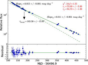
Figure 22. Fit of the bolometric light curve of SN 2013ej beyond +120 day with a broken exponential law. The solid line is the fitted model while the dashed lines are the extrapolation of each exponential models in either direction. The crossover is at break time, tbr = +183.4 ± 15.7 day.
Download figure:
Standard image High-resolution imageEquation (7) has been analogously applied to study the radial profile of surface brightness from the disks of galaxies (e.g., Muñoz-Mateos et al. 2013). The best-fit parameters are found to be,  days,
days,  days,
days,  and
and  with the
  from the fit to be 1.55. The slopes before and after the break point are obtained to be
 and
and 
 . While Slope1 is found to be much steeper, Slope2 is closer to the
  decay rate.
To see the effect of these two distinct decline behaviors on the initial Ni mass, we further fit the late-time bolometric light curve of SN 2013ej with the simple model described in Vinkó et al. (2004) and Valenti et al. (2008). This model assumes an optically thin ejecta heated by the radioactive decay of 56Ni and 56Co. The decay energy is emitted in the form of gamma rays and positrons, which may be partially trapped in the ejecta, thermalize and emerge again as low-energy (mostly optical or near-infrared) photons. The deposition function for the gamma rays at a given epoch t can be expressed as

where  is the optical depth for gamma rays in the whole ejecta. The timescale of the gamma ray optical depth decrease (Wheeler et al. 2015) is

where  is the gamma-ray opacity, Mej is the ejecta mass and C is a constant depending on the density distribution in the ejecta. For simplicity, we assumed a constant density ejecta, which implies
  . The deposition function for positrons,
  , takes the same form, except for the opacity. For the gamma-ray opacity, we adopted
  cm2 g−1 and for positrons, we set
  cm2 g−1 (e.g., Colgate et al. 1980; Valenti et al. 2008).
With these definitions, the late-time bolometric luminosity can be expressed as
where  is the initial mass of the radioactive 56Ni synthesized during the explosion,
  and
and  are the functions for the total energy input from the Ni- and Co-decay, respectively (see Branch & Wheeler 2016; Szalai et al. 2016 for further discussion). This equation corrects for the typographical error in the expression given by Valenti et al. (2008), and accounts for the partial trapping of both gamma-rays and positrons via the deposition functions given above. Since this light curve model assumes instantaneous release of the thermalized deposited energy from radioactive decay, without considering any photon diffusion unlike the model of Arnett (1980), it is applicable only when the ejecta is almost fully transparent in the optical, i.e., during the nebular phase.
The fit of Equation (11) to the bolometric lightcurve is plotted in Figure 23. We found that before +183 day, SN 2013ej exhibited a steeper decline in the bolometric light curve than the rate of the 56Co decay, as also found by Huang et al. (2015) and Bose et al. (2015a); however, our extended photometry, revealing a shallower decay rate, has an implication for both the gamma-ray opacities and the estimated Ni-mass. From the fit beyond the break point of +183 day, the values inferred for the initial nickel mass and the gamma-opacity timescale are 
 and
and  days. This timescale is significantly longer than the value of ∼173 day found by Bose et al. (2015a) from the data between +100 and +200 days. Our longer
  suggests that the light curve of SN 2013ej was probably not yet settled on the radioactive tail before +183 days. The Ni mass derived from the fit before break time,
 is consistent with our calculations above using methods of Bose et al. (2013) and Hamuy (2003), and with previous independent estimates by Huang et al. (2015) and Bose et al. (2013), both assuming full gamma-ray and positron trapping in about the same time window, but all those estimates are probably overestimates and the lower value derived by restricting the analysis beyond +183 day is more likely to be correct.
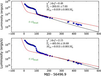
Figure 23. Fit of the radioactive decay model of Equation (11) to the bolometric light curve tail of SN 2013ej. Pre-break time and post break time lightcurves are fitted separately. The upper panel shows the fit taking data between +120 day and the break point at +183 day. The lower panel shows the same fit taking data beyond the break time. The leakage of both the gamma-rays and positrons were taken into account in the model (see text). The red line represents full trapping of gamma rays and positrons on both panels.
Download figure:
Standard image High-resolution image
7.2. Explosion Physical Parameters
To determine accurate explosion properties, a detailed hydrodynamic study is required. Recently, Huang et al. (2015) have done such a study while Bose et al. (2015a) use a semi-analytic approach following Arnett & Fu (1989). In order to make an approximate estimate, we use the approach of Litvinova & Nadyozhin (1985). Even though there are complications concerning radioactive heating effects, inclusion of higher explosion energies in the models, simple physical assumptions will still be useful to compare the explosion parameters with those of the more elaborate studies.
From plateau length ( ), the mid-plateau absolute V magnitude MV, and the corresponding expansion velocity, Litvinova & Nadyozhin (1985) derive the explosion energy, ejected mass, and pre-SN radius. For the plateau midpoint of SN 2013ej, we use
  where
where  is the epoch of peak brightness in V, estimated to be +15 day using Gaussian Process regression of V band data until +30 day, and
  is the epoch at which the plateau ends. It is nontrivial to precisely locate the end of the plateau. To determine this epoch, we again perform a Gaussian Process regression on the bolometric lightcurve from +80 day to +130 day, and determine the point of inflection from the obtained fit to be +109 day. We consider this to be the end of the plateau,
  . We therefore estimate a plateau of length 94 ± 7 with +62 day as the midpoint. The value of
  at +62 day is found to be 3800 ± 500 km s−1 from the fit described in Section 5.4, while MV is determined to be −16.47 ± 0.04 mag from linear interpolation of V magnitudes from +50 to +70 day. Using these values, we derive an explosion energy of
  erg, and a pre-SN radius of 250 ± 70
  based on Litvinova & Nadyozhin (1985). Bose et al. (2015a) find an explosion energy of
  erg and a pre-SN radius of 450
  . Huang et al. (2015) obtain values ranging over (0.7–2.1)
  erg and 230–600
  , respectively. Given the unstated uncertainty in Bose et al. (2015a), and the range from Huang et al. (2015), our calculations appear to be consistent with theirs. Our explosion energy and pre-SN radius are also in agreement with measurements with the SN IIP sample studies of Hamuy (2003) and Nadyozhin (2003), both of which use the same Litvinova & Nadyozhin (1985) relations we used.
We further use these relations to determine the ejecta mass, Mej, for SN 2013ej to be 13.8 ± 4.2  . Hamuy (2003) and Nadyozhin (2003) obtain Mej in the range 14–56
  and 10–30
  , repsectively, which encompasses our result. As for the explosion energy and pre-SN radius, the ejecta mass is highly sensitive to plateau length; better knowledge of the plateau length can yield more accurate results. For SN 2013ej specifically, Huang et al. (2015) and Bose et al. (2015a) find ejecta masses of 10.6
  and 12 ± 3
  , respectively. Nagy & Vinkó (2016) have derived an ejecta mass of 10.6
  from light curve modeling using a two-component model incorporating a dense inner core and an extended low mass envelope. These three estimates are all consistent with our measurement based on Litvinova & Nadyozhin (1985) relations. If we assume a remnant mass of 1.4
  , our measurement for the final pre-explosion progenitor mass is 15.2 ± 4.2
  .
.
Other measurements have been performed of SNe IIP progenitor mass in general or SN 2013ej specifically. Care is required in comparing progenitor masses, however, as some correspond to initial pre-explosion masses or ZAMS masses rather than the final pre-explosion progenitor mass we calculated above. Fraser et al. (2014), for instance, found the ZAMS mass to be in the 8–15.5  range for SN 2013ej, consistent with an M-type supergiant, from the archival HST images. Using X-ray observations, Chakraborti et al. (2016) derived a ZAMS mass of 14
  , accounting for the derived steady mass loss of 3 × 10⁻⁶
  yr−1 over the last 400 years. Given the uncertainties, these measurements are consistent with our final progenitor mass of 15.2 ± 4.2
  . For the general population of SNe IIP, Smartt et al. (2009) obtain a ZAMS mass range of 8–17
  . Use of nebular phase modeling (e.g., Jerkstrand et al. 2014) can also independently provide tighter constraints on the ZAMS masses of these events. However, studies involving hydrodynamical modeling (e.g., Utrobin & Chugai 2009, 2013) and stellar evolutionary models (e.g., Smartt et al. 2009), along with nebular spectra modeling, have shown conflicts in the derived initial mass of the progenitor stars.
8. DISCUSSION AND CONCLUSIONS
We present extensive photometry of the nearby SN 2013ej at UV, optical, and near-IR wavelengths. We also discuss well-sampled UV and optical spectroscopy from +8 to +135 day after explosion. SN 2013ej looks kinematically similar to other normal SNe IIP, but it also exhibits some unique features compared to a broader sample of SN IIP, such as a steep plateau, early appearance of strong Si ii  , and a flat Hα velocity profile. Such features hint at an intermediate class between SNe IIL and IIP, or probably a continuum in the distribution of these CC SNe. From a large sample of SNe II, Anderson et al. (2014) did not find any evidence of bimodality in the distributions of many photometric properties they studied based on the V band, thereby suggesting a continuum in the properties of SNe II.
SNe IIP show a wide range of plateau duration. Even the typical SNe IIP that exhibit flat plateaus, like SN 2006bp (<73 day, Quimby et al. 2007), SN 2013ab (∼80 day, Bose et al. 2015b), and SN 2003hn (∼75 day, Bersten et al. 2011), have shorter plateau duration compared to that of SN 2013ej. This indicates that the envelope mass of SN 2013ej is not atypical. The amount of decrease of luminosity from the end of the plateau to the radioactive phase may be related to production of Ni in the ejecta, but the value of  calculated for SN 2013ej is also not atypical of SNe IIP (e.g., Hamuy 2003; Bersten et al. 2011; Anderson et al. 2014).
Applying the t2 model to the early-time data, we estimated the shock breakout epoch of SN 2013ej to be MJD 56496.9 ± 0.3 days; however, the validity of a t2 model in the context of SNe IIP at very early time remains to be studied thoroughly. The late time light curve of SN 2013ej shows a broken decline behavior in all BV RI bands. While 
 , derived from the bolometric lightcurve before the break point at +183 day, is consistent with the previous studies (e.g., Bose et al. 2015a; Huang et al. 2015), this is perhaps overestimated by 50%. Beyond the break point, the slope is shallower, close to the expected rate of decay from 56Co of 0.01 mag day−1, resulting in
 . The characteristic timescale of trapping beyond the break point is much longer than that found earlier, possibly suggesting that SN 2013ej had not completely transitioned to the nebular phase before +183 day, or there was some excess flux from CSM interaction with ejecta or other source before that time.
Collecting multiband photometry from U through K for a few well-observed SNe from the literature, we establish a calibration relation between the UBV RI pseudo-bolometric flux and the UBV RIJHK bolometric flux, which may reach 2% precision. By performing a composite calibration, we showed that ROTSE or KAIT unfiltered measurements together with B − V information may also be sufficient to derive the bolometric luminosity with high precision for SN IIP. We also present a pseudo-bolometric BV RI calibration using a linear relation for unfiltered photometry. Given the position of SN 2013ej in relation to more typical SNe IIP and more rapidly declining SNe IIL, it would be interesting to explore the consistency of the bolometric calibration described here with a broader range of SNe II.
Even though SN 2013ej is mostly normal spectroscopically, the strong early appearance and subsequent evolution of the Si ii  line is rather unusual. Fe ii might also have appeared somewhat early. The velocity evolution of weak and strong ions resembles usual SN IIP behavior, but the flat H i velocity profile is consistently high among the SN IIP population. The correlation of
  and
and  as observed in a better-sampled study is also justified by SN 2013ej. One could expect somewhat different behavior with two components (photospheric and high velocity) of H i lines, but we do not see any HVFs in our spectra. SN 2013ej adds a valuable UV spectrum to the early-time UV sample, supporting the spectral homogeneity around +10 day after explosion. It is clear from the available sample that such homogeneity is not justified at earlier epochs. This also signifies the need of early time data.
By performing an EPM analysis of SN 2013ej, in combination with SN 2002ap, we estimated the distance to the host galaxy M74 to be  Mpc. Using the calibrated bolometric flux for unfiltered ROTSE data for SN 2013ej, we obtain a distance of
  Mpc, consistent with the previous derivation. Various physical parameters derived here and the findings from other studies of SN 2013ej are listed in Table 10. Generally, the values derived here from simple approximation models are consistent with other findings in the literature. Since we took the peak as the advent of plateau, we note that the expelled mass is likely overestimated while the radius could be underestimated.
Table 10. Calculated Physical Parameters of SN 2013ej
| Parameter | Bose et al. (2015a) | Huang et al. (2015) | Fraser et al. (2014) a | Valenti et al. (2014) | This Paper |
|---|---|---|---|---|---|
| Explosion Energy (1051 erg) | 2.3 | 0.7–2.1 | ⋯ | ⋯ | 0.9 ± 0.3 |
Progenitor Mass (M ) ) |
14.0 ± 3.0 | 12–13 | 8–15.5 | ⋯ |

|
Pre-SN Radius (R ) ) |
450 ± 112 | 230–600 | ⋯ | 400–600 | 250 ± 70 |
MNi (M ) ) |
0.019 ± 0.002 | 0.02 ± 0.01 | ⋯ | ⋯ | 0.013 ± 0.001 |
| Plateau Duration (Days) |

|

|
⋯ | ⋯ | 94 ± 7 |
| Distance Assumed (Mpc) | 9.57 ± 0.7 | 9.6 ± 0.7 | 9.1 ± 1.0 | 9.1 | ⋯ |
| Distance Measured (Mpc) | ⋯ | ⋯ | ⋯ | ⋯ |

|
Note.
aMass quoted is the ZAMS mass of the progenitor, elsewhere it is the final progenitor mass immediately before explosion.Download table as: ASCIITypeset image
Table 11. Rotse-IIIb Unfilterred Photometry of SN 2013ej
| MJD | ROTSE magnitude |
|---|---|
| 56498.38 | 13.32 (0.04) |
| 56498.41 | 13.22 (0.02) |
| 56504.36 | 12.30 (0.02) |
| 56504.37 | 12.08 (0.05) |
| 56505.32 | 12.30 (0.01) |
| 56506.40 | 12.23 (0.01) |
| 56506.32 | 12.24 (0.01) |
| 56507.38 | 12.22 (0.01) |
| 56507.29 | 12.21 (0.02) |
| 56508.39 | 12.20 (0.01) |
| 56508.32 | 12.21 (0.01) |
| 56510.40 | 12.16 (0.02) |
| 56510.31 | 12.19 (0.01) |
| 56511.27 | 12.20 (0.02) |
| 56512.27 | 12.21 (0.01) |
| 56513.38 | 12.17 (0.02) |
| 56513.31 | 12.20 (0.01) |
| 56516.25 | 12.24 (0.02) |
| 56517.32 | 12.21 (0.01) |
| 56518.33 | 12.23 (0.01) |
| 56520.41 | 12.27 (0.01) |
| 56521.36 | 12.28 (0.01) |
| 56521.28 | 12.27 (0.01) |
| 56522.36 | 12.30 (0.01) |
| 56523.35 | 12.36 (0.01) |
| 56523.30 | 12.31 (0.02) |
| 56524.37 | 12.38 (0.03) |
| 56525.34 | 12.39 (0.02) |
| 56526.25 | 12.32 (0.04) |
| 56527.32 | 12.54 (0.03) |
| 56530.24 | 12.49 (0.03) |
| 56531.18 | 12.48 (0.07) |
| 56533.28 | 12.58 (0.02) |
| 56534.34 | 12.59 (0.02) |
| 56534.26 | 12.60 (0.01) |
| 56535.31 | 12.61 (0.02) |
| 56536.25 | 12.63 (0.03) |
| 56537.31 | 12.66 (0.01) |
| 56537.24 | 12.64 (0.01) |
| 56538.19 | 12.66 (0.01) |
| 56539.32 | 12.70 (0.01) |
| 56539.22 | 12.69 (0.01) |
| 56540.31 | 12.72 (0.02) |
| 56540.23 | 12.71 (0.01) |
| 56541.23 | 12.75 (0.01) |
| 56542.21 | 12.76 (0.01) |
| 56543.31 | 12.77 (0.01) |
| 56543.23 | 12.78 (0.01) |
| 56549.36 | 12.88 (0.01) |
| 56549.23 | 12.86 (0.01) |
| 56563.21 | 13.07 (0.01) |
| 56563.16 | 13.04 (0.01) |
| 56565.28 | 13.11 (0.02) |
| 56565.20 | 13.07 (0.01) |
| 56567.24 | 13.11 (0.01) |
| 56568.23 | 13.14 (0.01) |
| 56568.17 | 13.14 (0.01) |
| 56569.24 | 13.14 (0.01) |
| 56569.11 | 13.09 (0.02) |
| 56570.26 | 13.19 (0.02) |
| 56570.19 | 13.17 (0.02) |
| 56571.27 | 13.18 (0.02) |
| 56571.19 | 13.19 (0.02) |
| 56572.24 | 13.20 (0.02) |
| 56572.21 | 13.21 (0.02) |
| 56573.16 | 13.22 (0.02) |
| 56574.27 | 13.25 (0.02) |
| 56575.22 | 13.26 (0.02) |
| 56575.16 | 13.24 (0.02) |
| 56576.20 | 13.27 (0.02) |
| 56576.18 | 13.27 (0.02) |
| 56577.37 | 13.27 (0.02) |
| 56578.12 | 13.30 (0.02) |
| 56586.38 | 13.59 (0.04) |
| 56586.34 | 13.54 (0.03) |
| 56587.18 | 13.55 (0.03) |
| 56587.18 | 13.59 (0.02) |
| 56588.18 | 13.61 (0.02) |
| 56588.17 | 13.61 (0.02) |
| 56589.19 | 13.63 (0.02) |
| 56589.15 | 13.62 (0.01) |
| 56590.24 | 13.68 (0.01) |
| 56590.16 | 13.66 (0.01) |
| 56591.19 | 13.72(0.01) |
| 56591.15 | 13.72 (0.01) |
| 56592.13 | 13.77 (0.01) |
| 56593.17 | 13.88 (0.03) |
| 56593.15 | 13.82 (0.03) |
| 56594.27 | 13.96 (0.04) |
| 56599.16 | 14.83 (0.02) |
| 56602.19 | 15.24 (0.03) |
| 56602.27 | 15.23 (0.03) |
| 56603.27 | 15.38 (0.04) |
| 56605.33 | 15.44 (0.05) |
| 56605.31 | 15.44 (0.04) |
| 56606.17 | 15.47 (0.04) |
| 56606.21 | 15.44 (0.04) |
| 56607.22 | 15.55 (0.06) |
| 56608.12 | 15.65 (0.07) |
| 56608.13 | 15.51 (0.04) |
| 56616.09 | 15.55 (0.08) |
| 56616.09 | 15.80 (0.07) |
| 56617.13 | 15.58 (0.08) |
| 56617.20 | 15.73 (0.04) |
| 56618.17 | 15.56 (0.13) |
| 56627.27 | 15.74 (0.09) |
| 56627.13 | 15.72 (0.15) |
| 56628.22 | 15.70 (0.24) |
| 56630.21 | 15.78 (0.11) |
| 56630.23 | 15.95 (0.07) |
| 56631.16 | 15.85 (0.07) |
| 56631.23 | 16.00 (0.07) |
| 56650.20 | 16.17 (0.12) |
| 56651.19 | 16.09 (0.08) |
| 56651.16 | 16.23 (0.11) |
| 56653.21 | 16.52 (0.14) |
| 56670.16 | 17.04 (0.50) |
| 56672.15 | 16.99 (0.34) |
| 56672.13 | 16.57 (0.15) |
| 56673.13 | 16.30 (0.07) |
| 56673.15 | 16.74 (0.14) |
| 56674.12 | 16.63 (0.12) |
| 56675.13 | 16.98 (0.22) |
| 56675.18 | 16.68 (0.11) |
| 56676.14 | 16.88 (0.19) |
| 56676.16 | 17.03 (0.19) |
| 56677.11 | 16.58 (0.19) |
| 56678.12 | 16.51 (0.12) |
| 56678.11 | 16.96 (0.16) |
| 56679.12 | 16.87 (0.14) |
| 56679.17 | 16.58 (0.07) |
| 56682.21 | 17.00 (0.21) |
| 56683.17 | 16.61 (0.11) |
| 56687.15 | 16.78 (0.15) |
Note. Photometric uncertainties are given inside parenthesis.
Table 12. BV RI photometry of SN 2013ej from Konkoly Observatory
| MJD | B | V | R | I |
|---|---|---|---|---|
| (mag) | (mag) | (mag) | (mag) | |
| 56505.5 | 12.64 (0.05) | 12.57 (0.02) | 12.49 (0.02) | 12.43 (0.02) |
| 56507.5 | 12.61 (0.01) | 12.52 (0.01) | 12.39 (0.01) | 12.36 (0.01) |
| 56510.5 | 12.66 (0.07) | 12.49 (0.07) | 12.35 (0.02) | 12.29 (0.01) |
| 56511.5 | 12.75 (0.08) | 12.51 (0.04) | 12.31 (0.01) | 12.26 (0.01) |
| 56512.5 | 12.78 (0.10) | 12.52 (0.03) | 12.31 (0.01) | 12.24 (0.02) |
| 56513.5 | 12.78 (0.06) | 12.48 (0.04) | 12.27 (0.04) | 12.21 (0.01) |
| 56516.5 | 12.99 (0.08) | 12.53 (0.02) | 12.31 (0.01) | 12.20 (0.02) |
| 56517.5 | 13.05 (0.04) | 12.54 (0.02) | 12.30 (0.02) | 12.19 (0.01) |
| 56521.5 | 13.38 (0.06) | 12.61 (0.02) | 12.32 (0.01) | 12.17 (0.01) |
| 56522.5 | 13.39 (0.05) | 12.64 (0.01) | 12.34 (0.01) | 12.19 (0.02) |
| 56535.5 | 14.15 (0.06) | 13.06 (0.01) | 12.61 (0.03) | 12.42 (0.04) |
| 56537.5 | 14.22 (0.01) | 13.11 (0.01) | 12.65 (0.01) | 12.43 (0.01) |
| 56540.5 | 14.42 (0.07) | 13.19 (0.07) | 12.70 (0.01) | 12.50 (0.01) |
| 56542.5 | 14.46 (0.03) | 13.23 (0.01) | 12.74 (0.01) | 12.51 (0.01) |
| 56543.5 | 14.49 (0.02) | 13.26 (0.01) | 12.76 (0.01) | 12.52 (0.01) |
| 56555.4 | 14.89 (0.12) | 13.48 (0.01) | 12.95 (0.06) | 12.66 (0.02) |
| 56563.4 | 15.01 (0.02) | 13.59 (0.03) | 13.03 (0.01) | 12.77 (0.01) |
| 56568.6 | 15.09 (0.01) | 13.69 (0.02) | 13.11 (0.01) | 12.84 (0.01) |
| 56573.6 | 15.29 (0.10) | 13.77 (0.01) | 13.19 (0.02) | 12.91 (0.01) |
| 56578.3 | 15.34 (0.06) | 13.88 (0.01) | 13.27 (0.01) | 12.98 (0.01) |
| 56591.4 | 15.93 (0.04) | 14.37 (0.01) | 13.67 (0.06) | 13.40 (0.01) |
| 56592.5 | 15.94 (0.05) | 14.41 (0.01) | 13.73 (0.03) | 13.43 (0.01) |
| 56597.3 | 16.65 (0.03) | 15.10 (0.01) | 14.28 (0.02) | 13.99 (0.01) |
| 56604.4 | 17.65 (0.04) | 16.24 (0.01) | 15.25 (0.02) | 14.92 (0.02) |
| 56628.2 | 17.95 (0.07) | 16.68 (0.01) | 15.63 (0.02) | 15.36 (0.01) |
| 56629.2 | 17.96 (0.06) | 16.70 (0.01) | 15.68 (0.03) | 15.43 (0.01) |
Note. Magnitudes are in the Vega-system, and uncertainties are given inside parentheses.
Download table as: ASCIITypeset image
Table 13. Sloan g'r'i'z' Photometry of SN 2013ej From Baja Observatory, Hungary
| MJD |

|

|

|

|
|---|---|---|---|---|
| (mag) | (mag) | (mag) | (mag) | |
| 56504.08 | 12.54 (0.06) | 12.61 (0.03) | 12.74 (0.09) | 13.01 (0.17) |
| 56505.07 | 12.49 (0.06) | 12.58 (0.04) | 12.63 (0.09) | 12.94 (0.23) |
| 56510.08 | 12.56 (0.10) | 12.44 (0.02) | 12.56 (0.02) | 12.68 (0.05) |
| 56512.09 | 12.60 (0.09) | 12.42 (0.02) | 12.55 (0.03) | 12.66 (0.05) |
| 56513.06 | 12.54 (0.04) | 12.40 (0.02) | 12.51 (0.04) | 12.62 (0.06) |
| 56516.06 | 12.64 (0.04) | 12.39 (0.02) | 12.49 (0.03) | 12.61 (0.05) |
| 56520.06 | 12.79 (0.04) | 12.41 (0.02) | 12.50 (0.02) | 12.59 (0.05) |
| 56521.06 | 12.84 (0.04) | 12.43 (0.02) | 12.51 (0.03) | 12.61 (0.05) |
| 56522.08 | 12.91 (0.04) | 12.45 (0.02) | 12.51 (0.05) | 12.63 (0.13) |
| 56535.00 | 13.48 (0.10) | 12.78 (0.04) | 12.90 (0.13) | 12.76 (0.07) |
| 56536.05 | 13.52 (0.05) | 12.75 (0.02) | 12.75 (0.03) | 12.75 (0.04) |
| 56539.07 | 13.61 (0.05) | 12.81 (0.02) | 12.83 (0.02) | 12.79 (0.06) |
| 56539.97 | 13.63 (0.03) | 12.83 (0.02) | 12.83 (0.02) | 12.77 (0.05) |
| 56541.92 | 13.69 (0.05) | 12.87 (0.02) | 12.87 (0.03) | 12.80 (0.06) |
| 56543.10 | 13.75 (0.03) | 12.88 (0.03) | 12.92 (0.06) | 12.85 (0.19) |
| 56543.95 | 13.75 (0.03) | 12.91 (0.02) | 12.91 (0.02) | 12.83 (0.04) |
| 56552.88 | 13.97 (0.08) | 13.05 (0.04) | 13.02 (0.05) | 12.92 (0.06) |
| 56558.91 | 14.06 (0.06) | 13.14 (0.04) | 13.13 (0.04) | 12.97 (0.06) |
| 56559.90 | 14.04 (0.08) | 13.14 (0.03) | 13.12 (0.03) | 12.99 (0.08) |
| 56568.88 | 14.25 (0.03) | 13.25 (0.03) | 13.26 (0.04) | 13.09 (0.06) |
| 56575.98 | 14.37 (0.05) | 13.41 (0.04) | 13.47 (0.05) | 13.19 (0.07) |
| 56576.95 | 14.61 (0.09) | 13.44 (0.03) | 13.44 (0.04) | 13.26 (0.06) |
| 56578.88 | 14.45 (0.08) | 13.50 (0.04) | 13.51 (0.03) | 13.29 (0.06) |
| 56586.87 | 14.73 (0.12) | 13.65 (0.04) | 13.67 (0.05) | 13.41 (0.10) |
| 56590.95 | 14.93 (0.06) | 13.79 (0.02) | 13.82 (0.03) | 13.53 (0.05) |
| 56592.96 | 15.25 (0.13) | 13.95 (0.04) | 14.00 (0.03) | 13.65 (0.04) |
| 56594.88 | 15.36 (0.03) | 14.14 (0.02) | 14.19 (0.02) | 13.79 (0.04) |
| 56596.03 | 15.78 (0.13) | 14.37 (0.06) | 14.45 (0.04) | 14.02 (0.10) |
| 56598.01 | 15.98 (0.06) | 14.67 (0.03) | 14.84 (0.05) | 14.19 (0.11) |
| 56603.90 | 16.88 (0.06) | 15.39 (0.02) | 15.54 (0.04) | 14.86 (0.07) |
| 56612.81 | 16.88 (0.34) | 15.70 (0.14) | 15.73 (0.10) | 15.22 (0.15) |
| 56626.97 | 17.21 (0.10) | 15.81 (0.04) | 16.04 (0.06) | 15.42 (0.11) |
| 56627.89 | 17.19 (0.06) | 15.78 (0.03) | 16.02 (0.04) | 15.40 (0.07) |
| 56628.75 | 17.36 (0.08) | 15.87 (0.04) | 16.03 (0.04) | 15.45 (0.08) |
| 56629.90 | 17.38 (0.08) | 15.83 (0.04) | 16.07 (0.04) | 15.40 (0.07) |
| 56636.81 | 17.28 (0.11) | 15.94 (0.05) | 16.21 (0.06) | 15.48 (0.08) |
| 56650.78 | 17.64 (0.10) | 16.11 (0.03) | 16.47 (0.06) | 15.82 (0.12) |
| 56660.84 | 17.95 (0.13) | 16.32 (0.05) | 16.78 (0.08) | 15.88 (0.14) |
| 56663.78 | 17.86 (0.12) | 16.39 (0.06) | 16.78 (0.09) | 15.99 (0.12) |
Note. Magnitudes are in the AB-system, and uncertainties are given inside parentheses.
Download table as: ASCIITypeset image
Table 14. KAIT Unfiltered and KAIT + Nickel BVRI Photometry of SN 2013ej
| MJD | Open CCD | B | V | R | I |
|---|---|---|---|---|---|
| (mag) | (mag) | (mag) | (mag) | (mag) | |
| 56498.45 | 13.30 (0.10) | ... | ... | ... | ... |
| 56499.44 | 12.95 (0.04) | ... | ... | ... | ... |
| 56504.39 | 12.29 (0.06) | 12.65 (0.06) | 12.68 (0.03) | 12.53 (0.03) | 12.52 (0.03) |
| 56507.51 | 12.23 (0.02) | 12.62 (0.03) | 12.54 (0.03) | 12.38 (0.03) | 12.37 (0.04) |
| 56509.52 | 12.24 (0.03) | 12.65 (0.10) | 12.57 (0.05) | 12.38 (0.02) | 12.37 (0.03) |
| 56515.51 | 12.21 (0.04) | 12.91 (0.04) | 12.51 (0.04) | 12.26 (0.03) | 12.17 (0.03) |
| 56516.51 | 12.21 (0.02) | ... | ... | ... | ... |
| 56519.48 | 12.29 (0.02) | 13.22 (0.04) | 12.61 (0.03) | 12.32 (0.02) | 12.20 (0.02) |
| 56520.51 | 12.33 (0.01) | 13.33 (0.04) | 12.64 (0.02) | 12.33 (0.02) | 12.23 (0.02) |
| 56522.50 | 12.36 (0.02) | 13.38 (0.04) | 12.64 (0.02) | 12.30 (0.01) | 12.20 (0.02) |
| 56523.45 | 12.41 (0.03) | 13.50 (0.03) | 12.68 (0.02) | 12.37 (0.02) | 12.23 (0.02) |
| 56524.50 | 12.40 (0.03) | 13.54 (0.04) | 12.70 (0.02) | 12.34 (0.02) | 12.21 (0.03) |
| 56525.34 | 12.45 (0.03) | 13.86 (0.09) | 12.87 (0.04) | 12.44 (0.03) | 12.33 (0.02) |
| 56527.38 | 12.52 (0.02) | 13.82 (0.04) | 12.85 (0.03) | 12.47 (0.04) | 12.32 (0.04) |
| 56530.49 | 12.57 (0.03) | 13.91 (0.04) | 12.92 (0.02) | 12.49 (0.02) | 12.32 (0.03) |
| 56532.53 | 12.62 (0.05) | ... | ... | ... | ... |
| 56533.43 | 12.67 (0.03) | 14.11 (0.04) | 13.01 (0.02) | 12.58 (0.02) | 12.40 (0.02) |
| 56534.49 | 12.64 (0.03) | 14.06 (0.03) | 13.00 (0.02) | 12.55 (0.02) | 12.37 (0.02) |
| 56536.40 | 12.72 (0.03) | 14.23 (0.03) | 13.08 (0.02) | 12.67 (0.02) | 12.46 (0.02) |
| 56537.45 | ... | 14.25 (0.12) | 13.10 (0.05) | 12.62 (0.02) | 12.35 (0.21) |
| 56539.41 | 12.77 (0.03) | 14.30 (0.03) | 13.12 (0.02) | 12.65 (0.02) | 12.46 (0.03) |
| 56540.41 | 12.78 (0.02) | 14.33 (0.03) | 13.15 (0.01) | 12.67 (0.02) | 12.48 (0.02) |
| 56541.36 | 12.84 (0.02) | ... | ... | ... | ... |
| 56542.42 | 12.82 (0.03) | 14.41 (0.03) | 13.19 (0.02) | 12.70 (0.02) | 12.48 (0.02) |
| 56543.38 | 12.87 (0.04) | 14.48 (0.04) | 13.22 (0.02) | 12.75 (0.02) | 12.53 (0.03) |
| 56545.48 | 12.86 (0.02) | 14.47 (0.04) | 13.23 (0.02) | 12.74 (0.02) | 12.54 (0.03) |
| 56546.41 | 12.88 (0.03) | 14.54 (0.04) | 13.30 (0.03) | 12.79 (0.04) | 12.56 (0.04) |
| 56548.39 | 12.92 (0.01) | 14.59 (0.03) | 13.31 (0.01) | 12.82 (0.01) | 12.57 (0.02) |
| 56549.40 | 12.92 (0.01) | 14.65 (0.03) | 13.33 (0.01) | 12.84 (0.01) | 12.61 (0.01) |
| 56550.43 | 12.95 (0.03) | 14.60 (0.03) | 13.32 (0.02) | 12.82 (0.02) | 12.59 (0.02) |
| 56551.45 | 12.97 (0.03) | 14.62 (0.03) | 13.33 (0.02) | 12.83 (0.02) | 12.60 (0.02) |
| 56552.29 | 12.98 (0.03) | 14.79 (0.08) | 13.44 (0.04) | 12.91 (0.04) | 12.70 (0.04) |
| 56553.36 | 13.02 (0.03) | ... | ... | ... | ... |
| 56559.37 | 13.08 (0.02) | 14.90 (0.04) | 13.50 (0.03) | 12.93 (0.04) | 12.72 (0.04) |
| 56562.31 | 13.13 (0.01) | 14.96 (0.03) | 13.56 (0.01) | 13.01 (0.01) | 12.77 (0.02) |
| 56563.40 | 13.15 (0.03) | ... | ... | ... | ... |
| 56564.37 | 13.15 (0.04) | 14.93 (0.04) | 13.58 (0.02) | 13.01 (0.02) | 12.76 (0.02) |
| 56566.49 | 13.14 (0.01) | 15.03 (0.05) | 13.59 (0.02) | 13.02 (0.01) | 12.78 (0.02) |
| 56567.38 | 13.18 (0.02) | ... | ... | ... | ... |
| 56569.29 | 13.21 (0.01) | ... | ... | ... | ... |
| 56570.39 | 13.21 (0.02) | 15.06 (0.03) | 13.65 (0.02) | 13.07 (0.02) | 12.82 (0.02) |
| 56571.31 | 13.22 (0.03) | ... | ... | ... | ... |
| 56572.35 | 13.25 (0.02) | 15.14 (0.04) | 13.70 (0.03) | 13.11 (0.03) | 12.86 (0.04) |
| 56573.35 | 13.22 (0.04) | ... | ... | ... | ... |
| 56574.35 | 13.27 (0.01) | 15.18 (0.05) | 13.74 (0.02) | 13.15 (0.01) | 12.89 (0.01) |
| 56575.37 | 13.30 (0.03) | ... | ... | ... | ... |
| 56576.33 | 13.33 (0.04) | ... | ... | ... | ... |
| 56577.38 | 13.34 (0.03) | 15.27 (0.04) | 13.77 (0.03) | 13.16 (0.02) | 12.94 (0.03) |
| 56579.33 | 13.36 (0.02) | ... | ... | ... | ... |
| 56580.32 | 13.41 (0.03) | 15.38 (0.04) | 13.87 (0.02) | 13.25 (0.02) | 13.02 (0.02) |
| 56581.24 | 13.44 (0.02) | ... | ... | ... | ... |
| 56587.32 | 13.61 (0.03) | 15.65 (0.05) | 14.10 (0.02) | 13.45 (0.02) | 13.20 (0.03) |
| 56588.33 | 13.64 (0.03) | ... | ... | ... | ... |
| 56589.32 | 13.70 (0.04) | ... | ... | ... | ... |
| 56590.32 | 13.72 (0.02) | 15.79 (0.05) | 14.23 (0.02) | 13.56 (0.02) | 13.32 (0.02) |
| 56591.31 | 13.74 (0.04) | ... | ... | ... | ... |
| 56592.30 | 13.89 (0.03) | ... | ... | ... | ... |
| 56596.29 | 14.30 (0.02) | 16.49 (0.06) | 14.91 (0.02) | 14.12 (0.01) | 13.85 (0.02) |
| 56597.27 | 14.45 (0.02) | ... | ... | ... | ... |
| 56598.28 | 14.63 (0.03) | ... | ... | ... | ... |
| 56599.26 | 14.83 (0.02) | 17.00 (0.08) | 15.54 (0.03) | 14.62 (0.03) | 14.35 (0.03) |
| 56600.27 | 15.03 (0.02) | ... | ... | ... | ... |
| 56601.26 | 15.16 (0.02) | ... | ... | ... | ... |
| 56603.31 | 15.38 (0.05) | ... | ... | ... | ... |
| 56604.27 | 15.38 (0.03) | ... | ... | ... | ... |
| 56605.28 | 15.42 (0.03) | ... | ... | ... | ... |
| 56606.27 | 15.45 (0.02) | 17.60 (0.09) | 16.36 (0.05) | 15.27 (0.04) | 14.95 (0.04) |
| 56608.22 | 15.59 (0.06) | ... | ... | ... | ... |
| 56615.27 | 15.55 (0.03) | 17.70 (0.29) | 16.55 (0.09) | 15.39 (0.03) | 15.06 (0.04) |
| 56618.22 | 15.63 (0.02) | 17.86 (0.22) | 16.57 (0.05) | 15.45 (0.02) | 15.17 (0.03) |
| 56619.26 | 15.64 (0.02) | ... | ... | ... | ... |
| 56620.25 | 15.65 (0.03) | ... | ... | ... | ... |
| 56621.28 | 15.68 (0.03) | 17.83 (0.18) | 16.65 (0.05) | 15.49 (0.03) | 15.24 (0.04) |
| 56622.23 | 15.72 (0.04) | ... | ... | ... | ... |
| 56624.23 | 15.72 (0.03) | 18.06 (0.22) | 16.65 (0.06) | 15.49 (0.03) | 15.24 (0.04) |
| 56625.25 | 15.74 (0.03) | ... | ... | ... | ... |
| 56626.21 | 15.72 (0.03) | ... | ... | ... | ... |
| 56627.23 | 15.77 (0.02) | 18.18 (0.25) | 16.70 (0.05) | 15.57 (0.03) | 15.31 (0.03) |
| 56628.25 | 15.78 (0.03) | ... | ... | ... | ... |
| 56629.25 | 15.81 (0.02) | ... | ... | ... | ... |
| 56630.20 | 15.83 (0.02) | 18.13 (0.18) | 16.72 (0.05) | 15.61 (0.03) | 15.37 (0.03) |
| 56631.18 | 15.88 (0.03) | ... | ... | ... | ... |
| 56632.17 | 15.89 (0.04) | ... | ... | ... | ... |
| 56634.24 | 15.90 (0.02) | ... | ... | ... | ... |
| 56635.15 | 15.92 (0.03) | ... | ... | ... | ... |
| 56636.17 | 15.97 (0.04) | ... | ... | ... | ... |
| 56641.20 | 15.98 (0.03) | 18.17 (0.30) | 16.88 (0.08) | 15.78 (0.03) | 15.54 (0.04) |
| 56643.20 | 16.02 (0.06) | ... | ... | ... | ... |
| 56645.24 | 16.03 (0.04) | ... | ... | ... | ... |
| 56647.23 | 16.06 (0.03) | ... | ... | ... | ... |
| 56648.21 | 16.08 (0.03) | 18.06 (0.20) | 17.13 (0.08) | 15.83 (0.03) | 15.63 (0.03) |
| 56649.20 | 16.10 (0.02) | ... | ... | ... | ... |
| 56650.18 | 16.11 (0.04) | ... | ... | ... | ... |
| 56651.19 | 16.15 (0.02) | 18.53 (0.36) | 17.05 (0.08) | 15.91 (0.03) | 15.68 (0.04) |
| 56653.18 | 16.18 (0.03) | ... | ... | ... | ... |
| 56655.15 | 16.23 (0.02) | 18.23 (0.30) | 17.12 (0.11) | 15.98 (0.04) | 15.80 (0.05) |
| 56656.17 | 16.24 (0.04) | ... | ... | ... | ... |
| 56658.15 | 16.30 (0.04) | 18.19 (0.21) | 17.15 (0.07) | 16.01 (0.03) | 15.80 (0.04) |
| 56660.15 | 16.39 (0.06) | ... | ... | ... | ... |
| 56662.17 | 16.32 (0.02) | ... | ... | ... | ... |
| 56668.12 | 16.46 (0.05) | ... | ... | ... | ... |
| 56669.12 | 16.41 (0.04) | ... | ... | ... | ... |
| 56673.15 | 16.52 (0.05) | ... | ... | ... | ... |
| 56674.11 | 16.48 (0.04) | 18.06 (0.25) | 17.47 (0.10) | 16.22 (0.05) | 15.99 (0.05) |
| 56676.16 | 16.55 (0.05) | ... | ... | ... | ... |
| 56677.13 | 16.54 (0.04) | ... | ... | ... | ... |
| 56679.13 | 16.56 (0.04) | 18.53 (0.41) | 17.54 (0.11) | 16.33 (0.05) | 16.11 (0.06) |
| 56682.12 | 16.62 (0.06) | ... | ... | ... | ... |
| 56684.13 | 16.61 (0.04) | 18.63 (0.30) | 17.66 (0.14) | 16.39 (0.05) | 16.21 (0.05) |
| 56708.12 | 16.87 (0.05) | ... | ... | ... | ... |
| 56710.13 | 16.94 (0.05) | ... | ... | ... | ... |
| Nickel Photometry | |||||
| 56505.4258 | ... | 12.37 (0.02) | 12.52 (0.01) | 12.43 (0.01) | 12.40 (0.01) |
| 56507.4883 | ... | 12.39 (0.01) | 12.50 (0.01) | 12.37 (0.01) | 12.32 (0.01) |
| 56523.3945 | ... | 13.40 (0.03) | 12.66 (0.01) | 12.36 (0.01) | 12.21 (0.01) |
| 56527.3398 | ... | 13.77 (0.04) | 12.79 (0.01) | 12.45 (0.01) | 12.26 (0.01) |
| 56531.3125 | ... | 13.90 (0.02) | 12.94 (0.01) | 12.50 (0.01) | 12.32 (0.01) |
| 56535.2969 | ... | 14.14 (0.02) | 13.05 (0.01) | 12.60 (0.01) | 12.39(0.01) |
| 56539.3242 | ... | 14.29 (0.02) | 13.17 (0.01) | 12.69 (0.01) | 12.45 (0.01) |
| 56541.3008 | ... | 14.38 (0.02) | 13.19 (0.01) | 12.72 (0.01) | 12.49 (0.01) |
| 56545.3008 | ... | 14.51 (0.02) | 13.27 (0.01) | 12.79 (0.01) | 12.52 (0.01) |
| 56548.2695 | ... | 14.59 (0.01) | 13.33 (0.01) | 12.84 (0.01) | 12.57 (0.01) |
| 56552.3516 | ... | 14.67 (0.02) | 13.41 (0.01) | 12.89 (0.01) | 12.63 (0.01) |
| 56555.3203 | ... | 14.80 (0.02) | 13.45 (0.01) | 12.92 (0.01) | 12.68 (0.02) |
| 56559.3086 | ... | 14.92 (0.01) | 13.52 (0.01) | 12.98 (0.01) | 12.72 (0.01) |
| 56562.3555 | ... | 15.00 (0.01) | 13.55 (0.01) | 13.00 (0.01) | 12.73 (0.01) |
| 56569.2930 | ... | 15.02 (0.03) | 13.54 (0.04) | 13.13 (0.04) | 12.78 (0.01) |
| 56573.3047 | ... | 15.27 (0.01) | 13.74 (0.01) | 13.17 (0.01) | 12.91 (0.01) |
| 56575.2656 | ... | 15.30 (0.01) | 13.78 (0.01) | 13.18 (0.01) | 12.91 (0.01) |
| 56578.3086 | ... | 15.42 (0.01) | 13.74 (0.01) | 13.25 (0.01) | 12.98 (0.01) |
| 56581.2812 | ... | 15.52 (0.01) | 13.94 (0.01) | 13.31 (0.01) | 13.04 (0.01) |
| 56585.3867 | ... | 15.67 (0.01) | 14.07 (0.01) | 13.43 (0.02) | 13.19 (0.03) |
| 56589.2656 | ... | 15.87 (0.01) | 14.24 (0.01) | 13.57 (0.01) | 13.28 (0.01) |
| 56599.2617 | ... | 17.07 (0.02) | 15.62 (0.01) | 14.70 (0.01) | 14.41 (0.01) |
| 56601.2734 | ... | 17.39 (0.01) | 15.97 (0.01) | 14.99 (0.01) | 14.67 (0.01) |
| 56605.2695 | ... | 17.68 (0.01) | 16.33 (0.01) | 15.28 (0.01) | 14.94 (0.05) |
| 56609.2656 | ... | 17.79 (0.02) | 16.44 (0.01) | 15.36 (0.01) | 15.04 (0.01) |
| 56626.2031 | ... | 18.07 (0.01) | 16.72 (0.01) | 15.60 (0.04) | 15.31 (0.08) |
| 56631.2148 | ... | 18.13 (0.03) | 16.79 (0.01) | 15.68 (0.01) | 15.39 (0.01) |
| 56635.2266 | ... | 18.17 (0.03) | 16.84 (0.01) | 15.73 (0.01) | 15.46 (0.01) |
| 56642.3359 | ... | 18.27 (0.16) | 16.78 (0.06) | 15.89 (0.03) | 15.53 (0.03) |
| 56645.2578 | ... | 18.41 (0.07) | 16.96 (0.02) | 15.89 (0.01) | 15.61 (0.01) |
| 56665.1875 | ... | 18.47 (0.04) | 17.32 (0.03) | 16.21 (0.02) | 15.93 (0.03) |
| 56670.1992 | ... | 18.66 (0.05) | 17.36 (0.02) | 16.27 (0.01) | 16.03 (0.01) |
| 56675.1914 | ... | 18.64 (0.04) | 17.44 (0.03) | 16.27 (0.06) | 16.03 (0.09) |
| 56678.1719 | ... | 18.66 (0.02) | 17.51 (0.02) | 16.32 (0.04) | 16.08 (0.08) |
| 56689.1250 | ... | 18.81 (0.03) | 17.63 (0.02) | 16.52 (0.01) | 16.25 (0.01) |
| 56705.1211 | ... | 18.96 (0.08) | 17.86 (0.03) | 16.71 (0.02) | 16.47 (0.04) |
| 56709.1250 | ... | 18.78 (0.06) | 17.78 (0.04) | 16.74 (0.02) | 16.51 (0.03) |
| 56724.1367 | ... | 19.17 (0.12) | 17.91 (0.04) | 16.88 (0.02) | 16.68 (0.03) |
| 56849.4336 | ... | 19.96 (0.19) | 19.27 (0.08) | 18.56 (0.04) | 18.34 (0.08) |
| 56852.4062 | ... | 20.65 (0.34) | 19.20 (0.08) | 18.46 (0.05) | 18.09 (0.06) |
| 56856.4141 | ... | 19.74 (0.15) | 19.21 (0.11) | 18.35 (0.06) | 18.41 (0.08) |
| 56894.3438 | ... | 20.31 (0.07) | 19.88 (0.04) | 19.21 (0.03) | 18.49 (0.07) |
| 56898.4609 | ... | 20.27 (0.05) | 20.02 (0.05) | 19.08 (0.05) | 18.73 (0.08) |
| 56916.4062 | ... | 20.49 (0.10) | 20.27 (0.07) | 19.55 (0.04) | 18.78 (0.06) |
| 56923.4453 | ... | 20.55 (0.06) | 20.09 (0.06) | 19.70 (0.05) | 19.03 (0.08) |
| 56931.3242 | ... | 20.86 (0.11) | 20.40 (0.07) | 19.84 (0.05) | 19.61 (0.15) |
| 56934.3633 | ... | 20.77 (0.14) | 20.21 (0.07) | 19.69 (0.07) | 19.21 (0.09) |
| 56937.2617 | ... | 21.06 (0.38) | 20.36 (0.20) | 19.59 (0.10) | 19.02 (0.10) |
| 56948.2344 | ... | 20.56 (0.11) | 20.41 (0.09) | 19.82 (0.06) | 19.70 (0.13) |
| 56958.2734 | ... | 20.72 (0.10) | 20.74 (0.10) | 20.13 (0.07) | 19.54 (0.12) |
Note. Magnitudes are in Vega system and uncertainties are given inside parenthesis.
Table 15. Optical and NIR Photometry of SN 2013ej from RATIR
| MJD | r | i | Z | Y | J | H |
|---|---|---|---|---|---|---|
| (mag) | (mag) | (mag) | (mag) | (mag) | (mag) | |
| 56500.0 | 13.0048 (0.02) | 13.2938 (0.02) | 13.3672 (0.02) | 13.3388 (0.02) | 13.8606 (0.05) | 14.1553 (0.07) |
| 56502.0 | 12.7652 (0.02) | 12.9600 (0.02) | 12.8912 (0.02) | 13.1330 (0.02) | 13.4210 (0.05) | 13.8766 (0.07) |
| 56503.0 | 12.6862 (0.02) | 12.8271 (0.02) | 12.8809 (0.02) | 13.0350 (0.02) | 13.3518 (0.05) | 13.6459 (0.07) |
| 56504.0 | 12.5889 (0.02) | 12.7816 (0.02) | 12.8486 (0.02) | 12.9499 (0.02) | 13.3239 (0.05) | 13.5421 (0.07) |
| 56505.0 | 12.5562 (0.02) | 12.7271 (0.02) | 12.8202 (0.02) | 12.9174 (0.02) | 13.2535 (0.05) | 13.4951 (0.07) |
| 56506.0 | 12.4911 (0.02) | 12.6626 (0.02) | 12.7144 (0.02) | 12.9752 (0.03) | 13.2002 (0.05) | 13.4347 (0.07) |
| 56508.0 | ... | ... | 12.7077 (0.02) | 12.8287 (0.03) | 13.1325 (0.05) | 13.3669 (0.07) |
| 56509.0 | 12.4615 (0.02) | 12.6214 (0.02) | 12.6969 (0.02) | 12.8081 (0.03) | ... | ... |
| 56510.0 | 12.4368 (0.02) | 12.6400 (0.02) | 12.6499 (0.02) | 12.7811 (0.03) | 13.0620 (0.05) | 13.3554 (0.07) |
| 56511.0 | 12.4306 (0.02) | 12.6635 (0.02) | 12.6288 (0.02) | 12.7200 (0.02) | 13.0414 (0.05) | 13.3042 (0.07) |
| 56512.0 | ... | 12.6110 (0.02) | 12.5960 (0.02) | 12.7521 (0.03) | 12.9975 (0.05) | 13.3020 (0.07) |
| 56517.0 | 12.4202 (0.02) | 12.5405 (0.02) | 12.5384 (0.02) | 12.6508 (0.03) | 12.8858 (0.05) | 13.1608 (0.07) |
| 56521.0 | ... | 12.6113 (0.02) | 12.5129 (0.02) | 12.6143 (0.02) | 12.8340 (0.05) | 13.0919 (0.07) |
| 56523.0 | 12.5081 (0.02) | 12.5448 (0.02) | 12.6007 (0.02) | 12.5571 (0.02) | 12.8797 (0.05) | 13.0437 (0.07) |
| 56541.0 | 12.8768 (0.02) | 12.8752 (0.02) | 12.7664 (0.02) | 12.7870 (0.03) | ... | ... |
| 56552.0 | 13.0548 (0.02) | 13.0406 (0.02) | 12.8758 (0.02) | 13.0518 (0.03) | 13.1447 (0.03) | 13.3756 (0.04) |
| 56559.0 | 13.1300 (0.02) | 13.1293 (0.02) | 12.9241 (0.02) | 13.1574 (0.03) | 13.2173 (0.03) | 13.4510 (0.04) |
| 56571.0 | 13.2975 (0.02) | 13.3096 (0.02) | 13.0648 (0.02) | 13.2636 (0.03) | 13.3389 (0.03) | 13.6176 (0.04) |
| 56578.0 | 13.4078 (0.02) | 13.4114 (0.02) | 13.1695 (0.02) | 13.5447 (0.03) | 13.4835 (0.03) | 13.7575 (0.04) |
| 56585.0 | 13.5672 (0.02) | 13.6186 (0.02) | 13.2659 (0.02) | 13.6321 (0.02) | 13.6367 (0.03) | 13.9024 (0.04) |
| 56588.0 | 13.7055 (0.02) | 13.7697 (0.02) | 13.4106 (0.02) | ... | 13.7585 (0.03) | 14.0406 (0.04) |
| 56589.0 | 13.7021 (0.02) | 13.8036 (0.02) | 13.4152 (0.02) | 13.8345 (0.02) | 13.7986 (0.03) | 14.1202 (0.04) |
| 56593.0 | 13.9689 (0.02) | 14.0149 (0.02) | 13.5742 (0.02) | 13.9862 (0.02) | 13.9705 (0.03) | 14.1668 (0.05) |
| 56595.0 | 14.1545 (0.02) | 14.2544 (0.02) | 13.7627 (0.02) | 14.2009 (0.02) | 14.1914 (0.03) | 14.4074 (0.05) |
| 56600.0 | 15.0154 (0.02) | 15.2823 (0.02) | 14.5393 (0.02) | 15.0502 (0.02) | 15.1220 (0.03) | 15.2142 (0.05) |
| 56604.0 | 15.3536 (0.02) | 15.5905 (0.02) | 14.8402 (0.02) | 15.4730 (0.02) | 15.3862 (0.03) | 15.5139 (0.03) |
| 56608.0 | 15.4652 (0.02) | 15.6747 (0.03) | 14.9609 (0.03) | 15.6256 (0.04) | 15.5659 (0.04) | 15.6812 (0.04) |
| 56623.0 | 15.6803 (0.02) | 15.9268 (0.02) | 15.2347 (0.03) | 15.8464 (0.04) | 15.8741 (0.06) | 15.9175 (0.14) |
Note. Magnitudes are in AB-system and photometric uncertainties are given inside parenthesis.
Download table as: ASCIITypeset image
This research was supported by NASA grant NNX10A196H (P.I. Kehoe), NSF grant AST-1109801 (P.I. Wheeler), and Hungarian OTKA grant NN 107637 (P.I. Vinko). J.M.S. is supported by an NSF Astronomy and Astrophysics Postdoctoral Fellowship under award AST-1302771. T.S. is funded by OTKA Postdoctoral Fellowship award PD 112325. K.S. has been supported by the Lendület-2009 program of the Hungarian Academy of Sciences and ESA PECS Contract No. 4000110889/14/NL/NDe. We also acknowledge support from the Hungarian Research Grants OTKA K-109276 and OTKA K-113117, as well as the Lendület-2009 and Lendület-2012 Program (LP2012-31) of the Hungarian Academy of Sciences. K.T. was supported by CONICYT through the FONDECYT grant 3150473 and by the Ministry of Economy, Development, and Tourism's Millennium Science Initiative through grant IC12009, awarded to the Millennium Institute of Astrophysics, MAS. L.M. is supported by the János Bolyai Research Scholarship of the Hungarian Academy of Sciences. A.V.F.'s group at U.C. Berkeley is supported by Gary & Cynthia Bengier, the Richard & Rhoda Goldman Fund, the Christopher R. Redlich Fund, the TABASGO Foundation, and NSF grant AST-1211916. Research at Lick Observatory is partially supported by a generous gift from Google. KAIT and its ongoing operation were made possible by donations from Sun Microsystems, Inc., the Hewlett-Packard Company, AutoScope Corporation, Lick Observatory, the NSF, the University of California, the Sylvia & Jim Katzman Foundation, and the TABASGO Foundation.
HET is a joint project of the University of Texas at Austin, the Pennsylvania State University, Stanford University, Ludwig-Maximilians-Universitat Munchen, and Georg-August-University Gottingen. The HET is named in honor of its principal benefactors, William P. Hobby and Robert E. Eberly. The Marcario Low Resolution Spectrograph is named for Mike Marcario of High Lonesome Optics who fabricated several optics for the instrument but died before its completion. The LRS is a joint project of the HET partnership and the Instituto de Astronomica de la Universidad Nacional Autonova de Mexico. The ROTSE-IIIb telescope is owned and supported by Southern Methodist University. We thank the staff at McDonald Observatory and Lick Observatory for their excellent work during the observations. We also thank U.C. Berkeley undergraduate students Minkyu Kim, Kevin Hayakawa, Haejung Kim, Heechan Yuk, Andrew Bigley, Goni Halevy, Samantha Cargill, Sahana Kumar, Kenia Pina, Kiera Fuller, Chadwick Casper, James Bradley, Philip Lu, Erin Leonard, Stephen Taylor, Jenifer Gross, Daniel Cohen, Michael Hyland, Kyle Blanchard, and Gary Li for their effort in taking Lick/Nickel data. We gratefully acknowledge Jon Mauerhan and Brad Tucker for helping obtain some of our optical spectra. We also thank the anonymous referee for many helpful discussions during the submission process of this paper.
We thank the RATIR project team and the staff of the Observatorio Astronomico Nacional on Sierra San Pedro Martir. RATIR is a collaboration between the University of California, the Universidad Nacional Autonoma de Mexico, NASA Goddard Space Flight Center, and Arizona State University, benefiting from the loan of an H2RG detector and hardware and software support from Teledyne Scientific and Imaging. RATIR, the automation of the Harold L. Johnson Telescope of the Observatorio Astronomico Nacional on Sierra San Pedro Martir, and the operation of both are funded through NASA grants NNX09AH71G, NNX09AT02G, NNX10AI27G, and NNX12AE66G, CONACyT grants INFR-2009-01-122785 and CB-2008-101958, UNAM PAPIIT grants IN113810 and IG100414, and a UCMEXUS-CONACyT grant.
Footnotes
- 15
- 16
- 17
IRAF is distributed by the National Optical Astronomy Observatories, which are operated by the Association of Universities for Research in Astronomy, Inc., under cooperative agreement with the National Science Foundation (NSF).
- 18
- 19
- 20
SExtractor and SWarp can be accessed from http://www.astromatic.net/software.
- 21
- 22
- 23
- 24