


ABSTRACT
We present early mid-ultraviolet and optical observations of Type IIn supernovae (SNe IIn) observed from 2007 to 2013. Our results focus on the properties of UV light curves: peak absolute magnitudes, temporal decay, and color evolution. During early times, this sample demonstrates that UV light decays faster than optical, and each event transitions from a predominantly UV-bright phase to an optically bright phase. In order to understand early UV behavior, we generate and analyze the sample's blackbody luminosity, temperature, and radius as the SN ejecta expand and cool. Since most of our observations were detected post maximum luminosity, we introduce a method for estimating the date of peak magnitude. When our observations are compared based on filter, we find that even though these SNe IIn vary in peak magnitudes, there are similarities in UV decay rates. We use a simple semi-analytical SN model in order to understand the effects of the explosion environment on our UV observations. Understanding the UV characteristics of nearby SNe IIn during an early phase can provide valuable information about the environment surrounding these explosions, leading us to evaluating the diversity of observational properties in this subclass.
Export citation and abstract BibTeX RIS
1. INTRODUCTION
Supernovae (SNe) are produced through two basic mechanisms: thermonuclear explosion of a white dwarf or gravitational collapse in the core of a massive star. SNe produced by the latter mechanism are referred to as core-collapse supernovae, and consist of SNe Ib, Ic, and II. The main distinction between Type Ib/c and Type II is the absence or presence of hydrogen lines in the spectra, respectively. Within the Type II SNe class there are recognized subclasses: Type IIb, Type II-L, Type II-P, and Type IIn.
Type II subclasses are characterized based on their photometric and spectral behavior (Filippenko 1997). Early Type IIb spectra reveal strong hydrogen emissions with no helium features, but hydrogen features diminish over time while helium emissions strengthen. Type II-L and Type II-P spectra display similar features, revealing only minor differences, and are further classified based on the behavior of their light curves. Type II-L light curves demonstrate a linear decline in brightness, while II-P light curves demonstrate a decline in brightness after maximum followed by a plateau phase. SNe IIn are distinguishable from SNe II-L and II-P based on their spectra. IIn spectra reveal very narrow emission lines, mainly hydrogen, superimposed on a broad emission component (Schlegel 1990). The growing consensus is that the light we observe from SNe IIn is the result of the explosive shock wave interacting with circumstellar material (CSM) surrounding the star prior to the explosion (e.g., Filippenko 1997; Gal-Yam et al. 2007). Some studies propose a massive luminous blue variable (LBV) as the progenitor star of a SN IIn (e.g., Gal-Yam et al. 2007; Smith et al. 2011a; Margutti et al. 2013).
Early photometric observations of SNe IIn have revealed a wide range of peak magnitudes and light-curve decay rates (e.g., Kiewe et al. 2012; Taddia et al. 2013). Based on the diversity of properties of IIn light curves, this subclass is commonly referred to as heterogeneous (e.g., Li et al. 2011; Moriya & Maeda 2014; Richardson et al. 2014). Properly comparing and characterizing early light curves based on maximum luminosites is difficult without well-constrained shock breakout dates. A systematic technique for comparing early light curves is needed to verify the true nature of IIn emissions. Early IIn observations are essential for understanding the physical properties of the SN explosion and the pre-explosion environment. The series of events following the SN explosion to the moment radiation is released is currently under investigation. In general, a shock wave is released after gravitational forces collapse the core of a massive star, accelerating the SN material. Kinetic energy in the shock is converted into thermal energy, and the stored energy is released in the form of radiation. The shocked, heated SN ejecta within the star travels through the stellar material toward an optically thinner, photospheric boundary. As the shock approaches the photosphere, the photons can escape, producing the X-ray and UV photons observed during the breakout.
For SNe IIn, it has been proposed that the interaction between the SN material and a cold dense shell, located at the photospheric boundary, is responsible for the unique IIn spectral and photometric features. The shell is formed when a significant amount of stellar material is released prior to core collapse. An increase in X-ray and UV production is observed as the shock front passes through the shell. The shock breakout is denoted as a sudden rise in luminosity, and due to the burst-like nature of this event it is rarely observed. Once the SN ejecta breaks through the surface of the star, it interacts with colder, less dense material, initiating the expansion phase, and the decay phase of the light curve. This description illustrates a basic shock-induced SN IIn and the evolution of the environment after the core collapses (e.g., Smith et al. 2008, 2010, 2011b; Taddia et al. 2013). The light observed from the explosion is dependent on the physical properties of these events, and these events are the result of the properties of the progenitor star.
Based on the basic sequence of events described, there are many parameters (e.g., progenitor mass and radii, mass loss rate, metallicity, energy of the explosion) involved in shaping the interaction between the SN ejecta and the CSM. Adding to the complexity of this environment, each individual property of the explosion and CSM may cover a range of values, which depend on the nature of the progenitor star and its mass loss history. IIn spectra have revealed a diversity of both mass loss rates and mass loss timescales. The timescale of a significant mass loss event can vary from months to decades before core collapse. These mass loss events are considered to be the result of violent eruptions or strong stellar winds, which then define the structure of the CSM (Mauerhan et al. 2013). Furthermore, IIn events are rare, making it difficult to statistically constrain explosion parameters based solely on observations.
Fortunately, in recent years, the number of IIn studies and follow-up programs has increased (e.g., Kiewe et al. 2012; Taddia et al. 2013; Ofek et al. 2014a). The Caltech Core-Collapse Project (CCCP) is one of the programs currently contributing to the advancement of IIn studies. CCCP has currently observed four SNe IIn in the optical and near-infrared range (Kiewe et al. 2012). Most IIn observations are ground-based; therefore, the focus of IIn studies is in the optical and near-IR wavelengths. During early times, SNe IIn have been shown to be extremely UV-bright, making them potential probes of star formation, and also excellent tools for quantifying the differences in absorption columns and metallicity (Cooke 2008; Cooke et al. 2009). The number of observations blue-ward of the U-band has fallen behind the number in the optical and infrared due to the lack of space-based UV resources. Since 2005, the Swift (Gehrels et al. 2004) Ultra-Violet/Optical Telescope (UVOT, Roming et al. 2005) has increased the number of early UV IIn observations.
In this paper, we present 10 IIn observations made in the UV and optical ranges, eight of which were captured no later than 20 days after the explosion and have more than five epochs. We discuss and analyze eight SNe observed by Swift UVOT and compare the sample to three SNe studied by the CCCP. In Section 2, we present the photometric observations. In Section 3, we analyze the properties of the light curves, the color evolution, and the physical properties of the photosphere for each SN. In Section 4, we present light curves produced using a semi-analytical model and compare the modeling results with our observations. In Section 5, we discuss our observations and modeling results. In Section 6, we summarize our results and discuss future work.
2. OBSERVATIONS
Our IIn UV observations were obtained using Swift UVOT. During early times, a typical UVOT exposure sequence consists of one 2 ks observation per day in all six UVOT filters: three ultraviolet and three optical filters (central wavelengths: uvw2, uvm2, uvm1, u, b, v; λc =  ,
,  ,
,  ,
,  ,
,  ,
,  , respectively; Poole et al. 2008). These early observations are made every other day in order to characterize an early UV light curve (Pritchard et al. 2014). If additional observation time is needed, the exposure time per observation is increased to 3 ks with observations made every three days. The data are collected, archived, and processed using the most recent version of the calibration database (Swift/UVOT CalDB version 20130118). Our IIn images are from the NASA HEASARC Swift Archive. We applied the 3'' source aperture photometric method used by Brown et al. (2009) and Pritchard et al. (2014), and the photometry results presented in Table 1 were corrected for Galactic extinction using the analytic model of Cardelli et al. (1989).
Table 1. Apparent Magnitudes of UVOT-observed IIn Supernovae
| Name | UT | Apparent Magnitudes | |||||
|---|---|---|---|---|---|---|---|
| JD2450000+ | uvw2 | uvm2 | uvw1 | u | b | v | |
| SN 2007pk | 4418.6 | 14.0(0.1) | 13.9(0.1) | 14.1(0.1) | 14.5(0.1) | 16.0(0.1) | 16.0(0.1) |
| 4420.2 | 14.4(0.2) | 14.1(0.1) | 14.2(0.1) | 14.6(0.1) | 16.0(0.1) | 15.9(0.1) | |
| 4420.7 | 14.6(0.2) | 14.2(0.1) | 14.3(0.1) | 14.7(0.1) | 15.9(0.1) | 16.0(0.1) | |
| 4421.7 | 14.9(0.2) | 14.5(0.1) | 14.5(0.1) | 14.7(0.1) | 16.0(0.1) | 15.9(0.1) | |
| 4425.1 | 15.4(0.2) | 15.1(0.1) | 15.0(0.1) | 14.9(0.1) | 16.0(0.1) | 15.9(0.1) | |
| 4429.6 | 16.3(0.2) | 16.1(0.1) | 15.8(0.1) | 15.2(0.1) | 16.1(0.1) | 15.9(0.1) | |
| 4433.9 | 17.3(0.3) | 16.9(0.2) | 16.5(0.2) | 15.6(0.1) | 16.3(0.1) | 16.1(0.1) | |
| 4436.9 | 17.6(0.1) | 17.7(0.3) | 17.1(0.2) | 16.0(0.1) | 16.4(0.1) | 16.1(0.1) | |
| 4440.8 | 17.8(0.1) | 17.9(0.1) | 17.5(0.3) | 16.4(0.2) | 16.5(0.1) | 16.2(0.1) | |
| 4451.9 | 17.8(0.1) | 18.0(0.1) | 17.9(0.1) | 17.3(0.2) | 17.1(0.2) | 16.5(0.1) | |
| SN 2008am | 4503.2 | ...(...) | 16.6(0.1) | ...(...) | 17.2(0.1) | 18.3(0.0) | 18.1(0.2) |
| 4504.1 | 18.4(0.3) | 17.1(0.3) | ...(...) | ...(...) | ...(...) | 18.1(0.2) | |
| 4512.5 | 17.4(0.3) | 16.8(0.2) | 17.5(0.2) | 17.6(0.2) | ...(...) | ...(...) | |
| 4539.4 | 18.8(0.3) | 18.1(0.2) | 18.4(0.1) | ...(...) | ...(...) | ...(...) | |
| SN 2009ip | 6183.9 | 19.4(0.2) | 19.2(0.2) | 18.4(0.1) | 17.5(0.1) | 18.0(0.1) | 18.3(0.1) |
| 6193.2 | 21.2(0.1) | 20.8(0.1) | 20.3(0.1) | 18.1(0.1) | 18.7(0.1) | 18.8(0.2) | |
| 6196.9 | 13.0(0.3) | 12.8(0.3) | 13.0(0.2) | 13.5(0.1) | 14.8(0.1) | 14.9(0.1) | |
| 6199.0 | 12.5(0.3) | 12.3(0.3) | 12.5(0.2) | 13.0(0.1) | 14.3(0.1) | 14.5(0.1) | |
| 6201.5 | 12.2(0.2) | 12.1(0.2) | 12.4(0.1) | 12.6(0.1) | 13.9(0.1) | 14.2(0.1) | |
| 6202.5 | 12.4(0.2) | 12.1(0.2) | 12.3(0.1) | 12.6(0.1) | 14.0(0.1) | 14.1(0.1) | |
| 6203.3 | 12.2(0.2) | 12.2(0.1) | 12.4(0.1) | 12.6(0.1) | 13.9(0.1) | 14.1(0.1) | |
| 6202.8 | 12.2(0.2) | 12.1(0.2) | 12.3(0.1) | 12.6(0.1) | 13.9(0.1) | 14.1(0.1) | |
| 6203.6 | 12.3(0.2) | 12.2(0.2) | 12.4(0.1) | 12.6(0.1) | 14.0(0.1) | 14.1(0.1) | |
| 6204.6 | 12.1(0.2) | 12.1(0.2) | 12.3(0.1) | 12.5(0.1) | 13.8(0.1) | 13.9(0.1) | |
| 6206.6 | 12.0(0.2) | 12.0(0.2) | 12.2(0.1) | 12.4(0.1) | 13.7(0.1) | 13.9(0.1) | |
| 6209.2 | 12.5(0.2) | 12.3(0.2) | 12.4(0.1) | 12.5(0.1) | 13.8(0.1) | 13.9(0.1) | |
| 6210.6 | 12.6(0.2) | 12.4(0.2) | 12.5(0.1) | 12.7(0.1) | 13.9(0.1) | 13.8(0.1) | |
| 6212.7 | 12.7(0.2) | 12.5(0.2) | 12.7(0.1) | 12.7(0.1) | 13.9(0.1) | 13.9(0.1) | |
| 6214.6 | 12.9(0.2) | 12.7(0.2) | 12.8(0.1) | 12.8(0.1) | 13.9(0.1) | 13.9(0.1) | |
| 6216.7 | 13.6(0.1) | 13.3(0.1) | 13.8(0.1) | 13.2(0.1) | 14.4(0.1) | 14.1(0.1) | |
| 6216.9 | 13.7(0.1) | 13.2(0.1) | 13.8(0.1) | 13.2(0.1) | 14.2(0.1) | 14.1(0.1) | |
| 6219.3 | 14.4(0.1) | 13.9(0.1) | 13.9(0.1) | 13.6(0.1) | 14.4(0.1) | 14.3(0.1) | |
| 6221.1 | 14.6(0.1) | 14.2(0.1) | 13.9(0.1) | 13.8(0.1) | 14.4(0.1) | 14.3(0.1) | |
| 6222.8 | 14.9(0.1) | 14.6(0.1) | 14.3(0.1) | 13.8(0.1) | 14.6(0.1) | 14.4(0.1) | |
| 6222.9 | 15.0(0.1) | 14.6(0.1) | 14.3(0.1) | 13.8(0.1) | 14.6(0.1) | 14.4(0.1) | |
| 6225.0 | 15.3(0.1) | 14.9(0.1) | 14.5(0.1) | 14.1(0.1) | 14.7(0.1) | 14.4(0.1) | |
| 6227.0 | 15.7(0.1) | 15.3(0.1) | 14.9(0.1) | 14.4(0.1) | 15.0(0.1) | 14.7(0.1) | |
| 6226.7 | 15.7(0.1) | 15.4(0.1) | 14.8(0.1) | 14.3(0.1) | 15.0(0.1) | 14.7(0.1) | |
| 6229.2 | 16.2(0.1) | 15.7(0.1) | 15.4(0.1) | 15.0(0.1) | 15.3(0.1) | 15.0(0.1) | |
| 6230.9 | 16.4(0.1) | 16.0(0.1) | 15.6(0.1) | 15.1(0.1) | 15.6(0.1) | 15.2(0.1) | |
| 6233.4 | 16.7(0.1) | 16.4(0.1) | 15.8(0.1) | 15.0(0.1) | 15.5(0.1) | 15.2(0.1) | |
| 6234.9 | 16.7(0.1) | 16.3(0.1) | 15.7(0.1) | 14.9(0.1) | 15.2(0.1) | 14.9(0.1) | |
| 6234.7 | 16.6(0.1) | 16.4(0.1) | 15.7(0.1) | 14.8(0.1) | 15.2(0.1) | 14.9(0.1) | |
| 6236.7 | 16.8(0.1) | 16.4(0.1) | 15.9(0.1) | 15.1(0.1) | 15.5(0.1) | 15.1(0.1) | |
| 6238.6 | 16.9(0.1) | 16.5(0.1) | 15.8(0.1) | 15.3(0.1) | 15.5(0.1) | 15.2(0.1) | |
| 6240.6 | 17.1(0.1) | 16.7(0.1) | 16.2(0.1) | 15.6(0.1) | 15.8(0.1) | 15.5(0.1) | |
| SN 2009ip | 6242.8 | 17.6(0.1) | 17.1(0.1) | 16.6(0.1) | 16.0(0.1) | 16.2(0.1) | 15.9(0.1) |
| 6244.9 | 18.3(0.1) | 17.4(0.1) | 17.1(0.1) | 16.5(0.1) | 16.7(0.1) | 16.2(0.1) | |
| 6247.4 | 18.3(0.1) | 17.7(0.1) | 17.3(0.1) | 16.7(0.1) | 16.6(0.1) | 16.2(0.1) | |
| 6248.6 | 18.3(0.1) | 17.7(0.1) | 17.1(0.1) | 16.5(0.1) | 16.5(0.1) | 16.1(0.1) | |
| 6250.6 | 18.5(0.1) | 18.2(0.1) | 17.9(0.1) | 16.8(0.1) | 17.0(0.1) | 16.3(0.1) | |
| 6253.1 | 19.0(0.2) | 18.7(0.1) | 17.7(0.1) | 17.0(0.1) | 17.1(0.1) | 16.2(0.1) | |
| 6254.6 | 19.1(0.2) | 18.8(0.1) | 17.8(0.1) | 17.4(0.1) | 17.1(0.1) | 16.6(0.1) | |
| SN 2010al | 5279.2 | 12.9(0.2) | 12.8(0.3) | 13.1(0.2) | 13.4(0.1) | 15.1(0.1) | 14.9(0.1) |
| 5284.4 | 14.3(0.1) | 13.9(0.1) | 13.9(0.1) | 13.9(0.1) | 15.3(0.1) | 15.4(0.1) | |
| 5286.1 | 14.8(0.1) | 14.4(0.1) | 14.2(0.1) | 14.1(0.1) | 15.3(0.1) | 15.5(0.1) | |
| 5288.1 | 15.1(0.1) | 14.7(0.1) | 14.6(0.1) | 14.2(0.1) | 15.5(0.1) | 15.4(0.1) | |
| 5289.9 | 15.7(0.1) | 15.4(0.1) | 14.9(0.1) | 14.5(0.1) | 15.7(0.1) | 15.6(0.1) | |
| 5291.7 | 16.3(0.2) | 16.0(0.1) | 15.4(0.1) | 14.8(0.1) | 15.7(0.1) | 15.7(0.1) | |
| 5293.7 | 16.4(0.2) | 16.0(0.1) | 15.6(0.1) | 14.8(0.1) | 15.8(0.1) | 15.7(0.1) | |
| 5296.0 | 16.9(0.2) | 16.7(0.2) | 16.3(0.1) | 15.1(0.1) | 15.9(0.1) | 15.7(0.1) | |
| 5297.8 | 17.3(0.3) | 16.5(0.1) | 16.6(0.2) | 15.6(0.1) | 16.1(0.1) | 16.3(0.1) | |
| 5299.7 | 17.7(0.1) | 17.3(0.3) | 16.8(0.2) | 15.8(0.1) | 16.5(0.1) | 16.2(0.2) | |
| 5304.3 | 17.8(0.1) | 17.8(0.1) | 17.7(0.1) | 17.2(0.3) | 17.5(0.2) | 16.7(0.2) | |
| SN 2010jl | 5505.6 | 13.9(0.1) | 13.7(0.1) | 13.5(0.1) | 13.2(0.1) | 13.9(0.1) | 13.8(0.1) |
| 5506.6 | 13.9(0.1) | 13.7(0.2) | 13.5(0.1) | 13.2(0.1) | 13.9(0.1) | 13.7(0.1) | |
| 5508.7 | 14.1(0.2) | 14.0(0.1) | 13.7(0.1) | 13.4(0.1) | 14.0(0.1) | 13.7(0.1) | |
| 5509.5 | 13.9(0.1) | 13.7(0.1) | 13.5(0.1) | 13.3(0.1) | 14.0(0.1) | 13.7(0.1) | |
| 5512.4 | 14.1(0.2) | 13.9(0.1) | 13.7(0.1) | 13.3(0.1) | 14.0(0.1) | 13.8(0.1) | |
| 5514.3 | 14.0(0.2) | 13.9(0.1) | 13.6(0.1) | 13.5(0.1) | 14.1(0.1) | 13.8(0.1) | |
| 5514.7 | 14.0(0.2) | 13.8(0.1) | 13.6(0.1) | 13.4(0.1) | 14.1(0.1) | 13.8(0.1) | |
| 5516.1 | 14.1(0.2) | 13.9(0.1) | 13.7(0.1) | 13.4(0.1) | 14.1(0.1) | 13.8(0.1) | |
| 5518.0 | 14.1(0.1) | 13.9(0.1) | 13.7(0.1) | 13.4(0.1) | 14.1(0.1) | 13.9(0.1) | |
| 5520.6 | 14.1(0.1) | 13.9(0.1) | 13.7(0.1) | 13.4(0.1) | 14.1(0.1) | 13.8(0.1) | |
| 5523.6 | 14.3(0.1) | 14.1(0.1) | 13.9(0.1) | 13.6(0.1) | 14.2(0.1) | 13.9(0.1) | |
| 5530.2 | 14.2(0.1) | 14.0(0.1) | 13.8(0.1) | 13.7(0.1) | 14.3(0.1) | 14.0(0.1) | |
| 5536.2 | 14.3(0.1) | 14.1(0.1) | 13.9(0.1) | 13.7(0.1) | 14.3(0.1) | 14.1(0.1) | |
| 5676.8 | 14.7(0.2) | 14.5(0.2) | 14.4(0.1) | 14.4(0.1) | 15.0(0.1) | 14.8(0.1) | |
| 5679.6 | 14.6(0.1) | 14.4(0.1) | 14.3(0.1) | 14.4(0.1) | 15.0(0.1) | 14.8(0.1) | |
| SN 2010jp | 5505.6 | 13.9(0.1) | 13.7(0.1) | 13.5(0.1) | 13.2(0.1) | 13.9(0.1) | 13.8(0.1) |
| 5506.6 | 13.9(0.1) | 13.7(0.2) | 13.5(0.1) | 13.2(0.1) | 13.9(0.1) | 13.7(0.1) | |
| 5508.7 | 14.1(0.2) | 14.0(0.1) | 13.7(0.1) | 13.4(0.1) | 14.0(0.1) | 13.7(0.1) | |
| 5509.5 | 13.9(0.1) | 13.7(0.1) | 13.5(0.1) | 13.3(0.1) | 14.0(0.1) | 13.7(0.1) | |
| 5512.4 | 14.1(0.2) | 13.9(0.1) | 13.7(0.1) | 13.3(0.1) | 14.0(0.1) | 13.8(0.1) | |
| 5514.3 | 14.0(0.2) | 13.9(0.1) | 13.6(0.1) | 13.5(0.1) | 14.1(0.1) | 13.8(0.1) | |
| 5514.7 | 14.0(0.2) | 13.8(0.1) | 13.6(0.1) | 13.4(0.1) | 14.1(0.1) | 13.8(0.1) | |
| 5516.1 | 14.1(0.2) | 13.9(0.1) | 13.7(0.1) | 13.4(0.1) | 14.1(0.1) | 13.8(0.1) | |
| 5518.0 | 14.1(0.1) | 13.9(0.1) | 13.7(0.1) | 13.4(0.1) | 14.1(0.1) | 13.9(0.1) | |
| 5520.6 | 14.1(0.1) | 13.9(0.1) | 13.7(0.1) | 13.4(0.1) | 14.1(0.1) | 13.8(0.1) | |
| 5523.6 | 14.3(0.1) | 14.1(0.1) | 13.9(0.1) | 13.6(0.1) | 14.2(0.1) | 13.9(0.1) | |
| 5530.2 | 14.2(0.1) | 14.0(0.1) | 13.8(0.1) | 13.7(0.1) | 14.3(0.1) | 14.0(0.1) | |
| 5536.2 | 14.3(0.1) | 14.1(0.1) | 13.9(0.1) | 13.7(0.1) | 14.3(0.1) | 14.1(0.1) | |
| SN 2011ht | 5838.6 | 20.1(0.1) | 19.7(0.1) | 18.8(0.2) | 17.6(0.1) | 17.0(0.1) | 16.3(0.1) |
| 5841.3 | 20.0(0.1) | 20.2(0.1) | 18.4(0.2) | 16.8(0.1) | 16.6(0.1) | 16.3(0.1) | |
| 5842.2 | 19.3(0.2) | 19.7(0.3) | 18.2(0.2) | 16.5(0.1) | 16.5(0.1) | 15.9(0.1) | |
| 5843.3 | 18.6(0.2) | 19.0(0.2) | 17.9(0.1) | 16.3(0.1) | 16.3(0.1) | 15.9(0.1) | |
| 5852.6 | 15.5(0.1) | 15.3(0.1) | 15.2(0.1) | 14.7(0.1) | 15.4(0.1) | 15.2(0.1) | |
| 5856.3 | 14.9(0.1) | 14.8(0.1) | 14.6(0.1) | 14.3(0.1) | 15.1(0.1) | 15.0(0.1) | |
| 5858.7 | 14.5(0.2) | 14.3(0.1) | 14.2(0.1) | 13.9(0.1) | 14.9(0.1) | 14.8(0.1) | |
| 5862.2 | 14.1(0.2) | 13.9(0.2) | 13.8(0.1) | 13.6(0.1) | 14.6(0.1) | 14.7(0.1) | |
| 5865.4 | 13.8(0.2) | 13.5(0.2) | 13.5(0.1) | 13.4(0.1) | 14.5(0.1) | 14.5(0.1) | |
| 5868.1 | 13.7(0.2) | 13.4(0.1) | 13.5(0.1) | 13.4(0.1) | 14.5(0.1) | 14.5(0.1) | |
| 5871.1 | 13.5(0.2) | 13.3(0.2) | 13.2(0.2) | 13.2(0.1) | 14.3(0.1) | 14.4(0.1) | |
| 5873.9 | 13.5(0.2) | 13.2(0.2) | 13.1(0.2) | 13.1(0.1) | 14.3(0.1) | 14.3(0.1) | |
| 5876.9 | 13.4(0.2) | 13.1(0.2) | 13.1(0.1) | 13.1(0.1) | 14.2(0.1) | 14.3(0.1) | |
| 5880.3 | 13.4(0.2) | 13.2(0.2) | 13.1(0.2) | 13.1(0.1) | 14.2(0.1) | 14.3(0.1) | |
| 5883.2 | 13.5(0.2) | 13.2(0.2) | 13.1(0.2) | 13.1(0.1) | 14.2(0.1) | 14.3(0.1) | |
| 5886.0 | 13.4(0.2) | 13.2(0.2) | 13.2(0.1) | 13.2(0.1) | 14.2(0.1) | 14.3(0.1) | |
| 5889.0 | 13.5(0.2) | 13.3(0.2) | 13.3(0.1) | 13.2(0.1) | 14.2(0.1) | 14.4(0.1) | |
| 5892.2 | 13.6(0.2) | 13.4(0.2) | 13.3(0.1) | 13.2(0.1) | 14.2(0.1) | 14.3(0.1) | |
| 5895.0 | 13.8(0.2) | 13.5(0.2) | 13.4(0.1) | 13.2(0.1) | 14.3(0.1) | 14.3(0.1) | |
| 5898.3 | 13.9(0.2) | 13.7(0.2) | 13.5(0.1) | 13.3(0.1) | 14.3(0.1) | 14.4(0.1) | |
| 5901.4 | 14.6(0.1) | 14.1(0.1) | 13.9(0.1) | 13.5(0.1) | 14.5(0.1) | 14.4(0.1) | |
| 5903.9 | 14.3(0.2) | 14.1(0.2) | 13.9(0.1) | 13.5(0.1) | 14.5(0.1) | 14.4(0.1) | |
| 5907.4 | 14.5(0.2) | 14.4(0.1) | 14.0(0.1) | 13.5(0.1) | 14.5(0.1) | 14.5(0.1) | |
| 5909.8 | 14.8(0.1) | 14.6(0.1) | 14.3(0.1) | 13.7(0.1) | 14.7(0.1) | 14.6(0.1) | |
| 5913.1 | 15.2(0.1) | 15.0(0.1) | 14.5(0.1) | 13.7(0.1) | 14.7(0.1) | 14.5(0.1) | |
| 5917.0 | 15.6(0.1) | 15.5(0.1) | 14.9(0.1) | 13.9(0.1) | 14.8(0.1) | 14.6(0.1) | |
| 5920.3 | 16.2(0.1) | 16.0(0.1) | 15.3(0.1) | 14.1(0.1) | 14.8(0.1) | 14.7(0.1) | |
| 5922.7 | 16.4(0.1) | 16.2(0.1) | 15.5(0.1) | 14.3(0.1) | 14.9(0.1) | 14.7(0.1) | |
| 5930.3 | 17.3(0.1) | 17.3(0.1) | 16.2(0.1) | 14.9(0.1) | 15.1(0.1) | 14.9(0.1) | |
| 5939.6 | 18.3(0.1) | 18.4(0.1) | 17.0(0.1) | 15.6(0.1) | 15.5(0.1) | 15.1(0.1) | |
| 5944.2 | 18.6(0.2) | 19.0(0.2) | 17.4(0.1) | 15.9(0.1) | 15.6(0.1) | 15.1(0.1) | |
| SN 2013L | 6321.4 | 14.1(0.1) | 14.0(0.1) | 14.0(0.1) | 14.2(0.1) | 15.6(0.1) | 15.8(0.3) |
| 6323.4 | 14.3(0.1) | 14.0(0.1) | 14.1(0.1) | 14.3(0.1) | 15.6(0.1) | 15.8(0.1) | |
| 6325.0 | 14.6(0.1) | 14.3(0.1) | 14.3(0.1) | 14.4(0.1) | 15.6(0.1) | 16.0(0.2) | |
| 6326.9 | 14.9(0.1) | 14.5(0.1) | 14.5(0.1) | 14.5(0.1) | 15.8(0.1) | 16.1(0.2) | |
| 6328.8 | 15.0(0.1) | 14.6(0.1) | 14.6(0.1) | 14.6(0.1) | 15.8(0.1) | 16.1(0.2) | |
| 6330.8 | 15.1(0.1) | 14.8(0.1) | 14.9(0.1) | 14.8(0.1) | 15.9(0.1) | 16.0(0.2) | |
| 6333.4 | 15.5(0.1) | 15.2(0.1) | 15.1(0.1) | 14.9(0.1) | 16.0(0.1) | 16.2(0.2) | |
| 6337.3 | 16.0(0.1) | 15.6(0.1) | 15.5(0.1) | 15.3(0.1) | 16.4(0.1) | 16.4(0.2) | |
| 6338.6 | 16.3(0.1) | 15.9(0.1) | 15.8(0.1) | 15.6(0.1) | 16.5(0.2) | 16.6(0.2) | |
| 6341.2 | 16.5(0.1) | 16.2(0.1) | 16.1(0.1) | 15.7(0.1) | 16.7(0.2) | 16.6(0.2) | |
| 6343.1 | 17.0(0.2) | 16.5(0.1) | 16.5(0.2) | 16.1(0.2) | 16.9(0.2) | 17.0(0.3) | |
| 6344.9 | 17.3(0.2) | 16.9(0.2) | 16.6(0.2) | 16.2(0.2) | 17.0(0.2) | 17.2(0.1) | |
| 6346.9 | 17.7(0.3) | 17.0(0.2) | 16.8(0.2) | 16.3(0.2) | 17.1(0.2) | 17.3(0.1) | |
| 6349.0 | 18.2(0.4) | 17.7(0.3) | 17.7(0.1) | 16.8(0.2) | 17.7(0.4) | 17.3(0.1) | |
| SN 2013by | 6407.4 | 11.1(0.2) | 11.0(0.1) | 11.2(0.1) | 11.5(0.1) | 13.0(0.1) | 13.3(0.1) |
| 6413.2 | 12.4(0.1) | 12.3(0.1) | 11.8(0.1) | 12.1(0.1) | 13.2(0.1) | 13.4(0.1) | |
| 6435.9 | 17.0(0.2) | 17.1(0.1) | 15.9(0.1) | 14.4(0.1) | 14.1(0.1) | 13.8(0.1) | |
| 6439.1 | 17.3(0.3) | 17.2(0.1) | 16.1(0.1) | 14.9(0.1) | 14.3(0.1) | 13.9(0.1) | |
| 6441.8 | 17.6(0.1) | 17.2(0.1) | 16.3(0.2) | 15.2(0.1) | 14.5(0.1) | 14.0(0.1) | |
| 6448.1 | 17.6(0.1) | 17.1(0.1) | 16.6(0.2) | 15.6(0.1) | 14.8(0.1) | 14.2(0.1) | |
| 6464.7 | 17.6(0.1) | 17.2(0.1) | 17.4(0.1) | 17.2(0.4) | 15.5(0.1) | 14.8(0.2) | |
| SN 2013fs | 6575.4 | 14.2(0.2) | 14.2(0.1) | 14.3(0.1) | 14.8(0.1) | 16.6(0.2) | 17.1(0.3) |
| 6576.4 | 14.7(0.2) | 14.5(0.1) | 14.6(0.1) | 14.9(0.1) | 16.6(0.2) | 16.9(0.2) | |
| 6576.9 | 14.6(0.2) | 14.5(0.1) | 14.6(0.1) | 14.9(0.1) | 16.5(0.2) | 16.8(0.2) | |
| 6577.8 | 14.9(0.1) | 14.7(0.1) | 14.7(0.1) | 14.9(0.1) | 16.5(0.2) | 16.8(0.2) | |
| 6579.2 | 15.3(0.1) | 15.0(0.1) | 15.0(0.1) | 15.1(0.1) | 16.6(0.2) | 16.8(0.2) | |
| 6580.6 | 15.6(0.1) | 15.4(0.1) | 15.3(0.1) | 15.3(0.1) | 16.7(0.2) | 16.9(0.2) | |
| 6584.1 | 16.5(0.1) | 16.3(0.1) | 16.1(0.1) | 15.7(0.1) | 17.0(0.2) | 17.1(0.3) | |
| 6584.9 | 16.7(0.1) | 16.6(0.1) | 16.2(0.1) | 15.8(0.1) | 17.4(0.3) | 17.4(0.1) | |
| 6586.0 | 16.9(0.1) | 16.9(0.1) | 16.4(0.1) | 16.0(0.1) | 17.4(0.3) | 17.3(0.3) | |
| 6586.9 | 17.1(0.2) | 17.0(0.1) | 16.7(0.1) | 16.1(0.2) | 17.6(0.3) | 17.6(0.1) | |
| 6588.1 | 17.4(0.2) | 17.4(0.2) | 16.8(0.1) | 16.3(0.2) | 17.7(0.3) | 17.6(0.1) | |
| 6589.0 | 17.7(0.2) | 17.4(0.2) | 17.1(0.2) | 16.4(0.2) | 17.8(0.3) | 17.6(0.1) | |
| 6589.9 | 17.9(0.2) | 17.9(0.2) | 17.3(0.2) | 16.7(0.2) | 17.9(0.1) | 17.6(0.1) | |
| 6591.0 | 18.2(0.3) | 18.3(0.3) | 17.6(0.2) | 16.8(0.2) | 17.8(0.1) | 17.7(0.1) | |
Table 2 lists the 10 UVOT-observed SNe IIn. The light curves for these SNe are shown in Figure 1. For each SN, Table 2 provides basic properties: host galaxy, R.A. and Decl., redshift, distance, date of discovery, estimated shock breakout date, and E(B – V) extinction. The shock breakout dates presented are from the literature. If a shock breakout date has not been published, we use upper-limit observations to predict the shock breakout date. We define the shock breakout date as the midpoint between the upper limit observation and the discovery date. The Galactic extinction for each SN was computed using E(B – V) values from Schlegel et al. (1998). The host extinction values in the table are from the literature, and the values are applied using the analytic model of Cardelli et al. (1989) as well. If host extinction values and upper-limit host extinction values are not available in the literature, we fit for the host extinction value using an upper limit of E(B – V) = 0.3 and follow the model discussed in Pritchard et al. (2014).
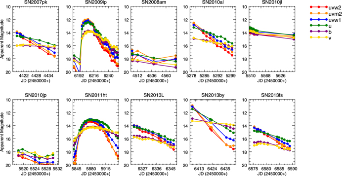
Figure 1. Light curves for 10 SNe IIn observed by UVOT in three UV filters, and the u, b, and v bands. Two SNe were observed early enough to detect the rise to the peak in all six filters: SN 2009ip and SN 2011ht.
Download figure:
Standard image High-resolution imageTable 2. Properties of UVOT-observed Type IIn Supernovae
| Name | Host Galaxy | R.A. | Decl. | Redshift | Distance | Discovery | Shock Breakout | E(B – V) | E(B – V) | References |
|---|---|---|---|---|---|---|---|---|---|---|
| (h m s) | (deg m s) | z | (Mpc) | 2450000+d | 2450000+e | MWb | Hostc | |||
| SN 2007pka | NGC 579 | 01 31 47.07 | +33 36 54.1 | 0.0167 | 66.90 | 4414.2 | 4412.2 ± 2.5 | 0.046 | <0.13 | (1), (2) |
| SN 2009ipa | NGC 7259 | 22 23 08 | −28 56 52.4 | 0.0059 | 20.4 | 6132.0 | 6132.0 | 0.018 | 0.01 | (5), (6), (7) |
| SN 2010ala | UGC4286 | 08 14 15.95 | +18 26 18.0 | 0.0170 | 73.4 | 5268.5 | 5251.0 ± 17 | 0.041 | ⋯ | (8) |
| SN 2010jpa | NGC 2207 | 06 16 30.63 | −21 24 36.0 | 0.0090 | 38.02 | 5511.8 | 5501.0 ± 9 | 0.087 | <0.16 | (14), (15), (16) |
| SN 2011hta | NGC 5460 | 10 08 10.59 | +51 50 57.0 | 0.0040 | 19.90 | 5833.6 | 5833.6 | 0.009 | 0.04 | (17)–(20) |
| SN 2013L | ESO 216-39 | 11 45 29.5 | −50 35 53 | 0.0160 | 73.20 | 6314.0 | 6304.0 ± 9 | 0.118 | ... | (21) |
| SN 2013by | ESO 138-G10 | 16 59 02.4 | −60 11 42 | 0.0040 | 16.9 | 6406.5 | 6396.5 ± 9 | 0.194 | ... | (22) |
| SN 2013fs | NGC 7610 | 23 19 44.67 | 10 11 04.5 | 0.0120 | 50.3 | 6574.5 | 6566.5 ± 7.5 | 0.035 | ... | (23) |
Notes.
aThe R.A., decl., redshift, and distance values for these SNe are from Pritchard et al. (2014). bThe Galactic extinction E(B – V) is the galactic line-of-sight reddening in the direction of the SNe using Schlafly & Finkbeiner (2011). cThe line-of-sight reddening values for the host galaxy are from the literature or generated using the model described in Pritchard et al. (2014). dThe discovery date is the Julian Date of the supernova discovery image found in the literature. eThe Julian Date of shock breakout is from the literature or it is defined as the midpoint between any reported pre-explosion observations of the SN and the discovery date.References. (1) Parisky & Li (2007), (2) Pritchard et al. (2012), (3) Yuan et al. (2008), (4) Chatzopoulos et al. (2011), (5) Maza et al. (2009), (6) Margutti et al. (2013), (7) Prieto et al. (2013), (8) Rich (2010), (9) Newton & Puckett (2010), (10) Benetti et al. (2010), (11) Yamanaka et al. (2010), (12) Stoll et al. (2011), (13) Ofek et al. (2014b), (14) Maza et al. (2010), (15) Challis et al. (2010), (16) Smith et al. (2012), (17) Boles et al. (2011), (18) Roming et al. (2012), (19) Humphreys et al. (2012), (20) Mauerhan et al. (2013), (21) Monard et al. (2013), (22) Parker et al. (2013), (23) Nakano et al. (2013).
Download table as: ASCIITypeset image
A sample of previously studied SNe from the CCCP are used for comparison. This literature sample includes SN 2005cl, SN 2005cp, and SN 2005db (Kiewe et al. 2012). The comparison sample is shown in Figure 2. The photometry for the comparison SNe was corrected for Galactic extinction and host galaxy extinction (Kiewe et al. 2012).
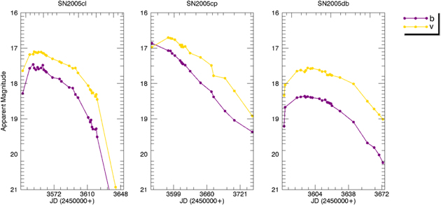
Figure 2. Light curves of three comparison SNe from CCCP observed in the b and v bands. SN 2005cl and SN 2005db were captured early enough to detect a slight rise to peak in both filters. SN 2005cp shows a slight rise to peak in the v band.
Download figure:
Standard image High-resolution image3. RESULTS
In previous IIn studies, early ground-based observations have revealed a wide range of peak magnitudes. The shock breakout is not typically observed during these early observations and the "true" peak magnitude is usually unknown. The uncertainty associated with the observed peak magnitude introduces systematic error when comparing IIn events based on peak luminosity.
IIn photometric observations have also been revealed as extremely UV-bright events. This study focuses on the early behavior of UV light curves, and our optical observations are used for comparison with ground-based observations. In order to verify whether IIn events are truly heterogenous, we investigate the early properties of the light curves: peak absolute magnitudes, temporal decay, and color evolution. The rise to maximum brightness is believed to be the product of the SN ejecta interacting with the CSM, and therefore peak magnitudes reveal information about the explosion, the SN ejecta, and the CSM. The decay of the light curve represents the SN expansion phase. The color evolution is used to analyze the change in flux over time. A detailed analysis of the UV observational properties of the sample, as a whole and for each individual SN, will aid the current understanding of the physics behind SNe IIn.
Since our study focuses on the early behavior of the UV light curves of nearby SNe, only eight out of the ten UVOT-observed SNe were chosen to conduct a systematic and statistically significant comparison. The criterion for SN selection was based on the number of observations and how long after shock breakout the SN was discovered. The two SNe excluded from the final sample are SN 2008am and SN 2010jl. When compared to the other SNe, SN 2008am was observed at higher redshift, z = 0.2380, and the first UVOT observation was approximately 37 days after shock breakout, with an average of three epochs per filter (Yuan et al. 2008). This SN does not have a sufficient number of observations to analyze the decay rate, and based on null observations, it was observed long after peak UV and optical magnitude. Similarly, SN 2010jl was discovered approximately 40 days after shock breakout and has a temporal decay of 0.01 in the UV and 0.01 in the optical, confirming that this SN was also observed long after maximum light (Benetti et al. 2010; Newton & Puckett 2010; Yamanaka et al. 2010).
After removing these SNe, we note that during early observations the SNe in our tailored sample appear to be 2 mag brighter at UV wavelengths than optical. In Figure 1, these SNe display a rapid UV decay relative to the optical bands, and the SNe eventually transition from being UV-bright to being optically bright. For both the UVOT-observed SNe and the comparison SNe, Table 3 lists the peak absolute magnitudes calculated using the distance values from Table 2, and Table 4 lists the temporal decay. We analyze the color evolution for each SN, and the color evolution rate, or the slope of the color evolution trends, is included in Table 5.
Table 3. Peak Absolute Magnitudes of the UVOT-observed and CCCP Sample
| Name | Peak Absolute Magnitude | |||||
|---|---|---|---|---|---|---|
| uvw2 | uvm2 | uvw1 | u | b | v | |
| SN 2007pk | −20.15(0.1) | −20.27(0.1) | −20.03(0.1) | −19.60(0.1) | −18.21(0.1) | −18.25(0.1) |
| SN 2009ip | −19.51(0.2) | −19.57(0.1) | −19.40(0.1) | −19.11(0.1) | −17.82(0.1) | −17.73(0.1) |
| SN 2010al | −21.32(0.2) | −21.45(0.3) | −21.17(0.2) | −20.90(0.1) | −19.24(0.1) | −19.37(0.1) |
| SN 2010jp | −14.29(0.1) | −14.38(0.1) | −14.89(0.1) | −15.28(0.1) | −14.50(0.1) | −14.78(0.1) |
| SN 2011ht | −18.13(0.2) | −18.38(0.2) | −18.43(0.1) | −18.38(0.1) | −17.29(0.1) | −17.24(0.1) |
| SN 2013L | −20.22(0.1) | −20.37(0.1) | −20.33(0.1) | −20.13(0.1) | −18.73(0.1) | −18.57(0.3) |
| SN 2013by | −20.02(0.2) | −20.12(0.1) | −19.96(0.1) | −19.62(0.1) | −18.15(0.1) | −17.80(0.1) |
| SN 2013fs | −19.27(0.2) | −19.35(0.1) | −19.18(0.1) | −18.71(0.1) | −17.04(0.2) | −16.74(0.3) |
| SN 2005cl | ... | ... | ... | ... | −18.07 | −18.43 |
| SN 2005cp | ... | ... | ... | ... | −18.54 | −18.70 |
| SN 2005db | ... | ... | ... | ... | −15.51 | −16.31 |
| Average | −19.11 | −19.24 | −19.17 | −18.97 | −17.56 | −17.63 |
| Std. Dev | 2.15 | 2.15 | 1.91 | 1.69 | 1.42 | 1.30 |
| Mediana | −19.510 | −19.567 | −19.397 | −19.114 | −17.819 | −17.729 |
| MADb | 0.710 | 0.802 | 0.930 | 0.731 | 0.780 | 0.838 |
Notes.
aMedian value for the peak values. bMedian absolute deviation (MAD) value is the median of the absolute value of the difference between the peak values and the median.Download table as: ASCIITypeset image
Table 4. Temporal Decay of the UVOT-observed and CCCP Sample
| Name | Temporal Decay (mag/day) | |||||
|---|---|---|---|---|---|---|
| w2 | m2 | w1 | u | b | v | |
| SN 2007pk | 0.197(0.007) | 0.207(0.003) | 0.164(0.004) | 0.076(0.004) | 0.028(0.003) | 0.018(0.005) |
| SN 2009ip | 0.159(0.005) | 0.149(0.005) | 0.126(0.004) | 0.104(0.004) | 0.071(0.004) | 0.064(0.003) |
| SN 2010al | 0.229(0.008) | 0.217(0.011) | 0.193(0.007) | 0.117(0.006) | 0.063(0.005) | 0.058(0.007) |
| SN 2010jp | 0.120(0.016) | 0.121(0.024) | 0.144(0.029) | 0.077(0.057) | 0.054(0.018) | 0.035(0.028) |
| SN 2011ht | 0.055(0.005) | 0.057(0.005) | 0.045(0.004) | 0.025(0.002) | 0.021(0.001) | 0.012(0.001) |
| SN 2013L | 0.134(0.005) | 0.124(0.004) | 0.115(0.003) | 0.085(0.004) | 0.070(0.003) | 0.058(0.005) |
| SN 2013by | 0.188(0.011) | 0.187(0.014) | 0.155(0.006) | 0.106(0.001) | 0.043(0.002) | 0.018(0.001) |
| SN 2013fs | 0.245(0.005) | 0.251(0.006) | 0.204(0.004) | 0.124(0.004) | 0.124(0.007) | 0.083(0.008) |
| SN 2005cl | ...(...) | ...(...) | ...(...) | ...(...) | 0.007(0.001) | 0.011(0.001) |
| SN 2005cp | ...(...) | ...(...) | ...(...) | ...(...) | 0.013(0.002) | 0.011(0.001) |
| SN 2005db | ...(...) | ...(...) | ...(...) | ...(...) | 0.010(0.001) | 0.009(0.001) |
| Average | 0.167 | 0.165 | 0.144 | 0.088 | 0.045 | 0.034 |
| Std. Dev | 0.061 | 0.063 | 0.050 | 0.034 | 0.035 | 0.027 |
| Mediana | 0.188 | 0.187 | 0.154 | 0.104 | 0.043 | 0.018 |
| MADb | 0.054 | 0.063 | 0.037 | 0.019 | 0.027 | 0.009 |
| Without SN 2011ht and Comparison SNe | ||||||
| Average | 0.181 | 0.179 | 0.157 | 0.099 | 0.065 | 0.048 |
| Std. Dev | 0.046 | 0.049 | 0.033 | 0.019 | 0.030 | 0.025 |
| Mediana | 0.188 | 0.187 | 0.155 | 0.104 | 0.054 | 0.035 |
| MADb | 0.041 | 0.038 | 0.029 | 0.019 | 0.027 | 0.025 |
Notes.
aMedian value for the magnitude decay values..
bMedian absolute deviation (MAD) value is the median of the absolute value of the difference between the magnitude decay values and the median.Download table as: ASCIITypeset image
Table 5. Color Evolution of the UVOT-observed and CCCP Sample
| Name | Color Evolution per day | |||||
|---|---|---|---|---|---|---|
| uvw2 – uvm2 | uvm2 – v | uvw1 – u | u – v | b – v | uvw2 – uvw1 | |
| SN 2007pk | −0.010(0.009) | 0.198(0.006) | 0.088(0.003) | 0.067(0.003) | 0.015(0.003) | 0.032(0.010) |
| SN 2009ip | 0.009(0.003) | 0.090(0.025) | 0.022(0.013) | 0.045(0.007) | 0.012(0.002) | 0.033(0.009) |
| SN 2010al | 0.012(0.008) | 0.159(0.016) | 0.076(0.007) | 0.059(0.006) | 0.006(0.008) | 0.036(0.012) |
| SN 2010jp | 0.001(0.016) | 0.090(0.039) | 0.066(0.012) | 0.050(0.036) | 0.012(0.027) | −0.025(0.017) |
| SN 2011ht | −0.002(0.005) | 0.047(0.018) | 0.025(0.006) | 0.011(0.007) | 0.005(0.002) | 0.010(0.006) |
| SN 2013L | 0.010(0.003) | 0.066(0.003) | 0.029(0.002) | 0.027(0.003) | 0.006(0.004) | 0.020(0.004) |
| SN 2013by | 0.002(0.009) | 0.170(0.015) | 0.049(0.007) | 0.088(0.001) | 0.026(0.001) | 0.035(0.010) |
| SN 2013fs | −0.006(0.007) | 0.182(0.008) | 0.081(0.005) | 0.055(0.006) | 0.038(0.004) | 0.040(0.004) |
| SN 2005cl | ...(...) | ...(...) | ...(...) | ...(...) | 0.014(0.001) | ...(...) |
| SN 2005cp | ...(...) | ...(...) | ...(...) | ...(...) | −0.001(0.003) | ...(...) |
| SN 2005db | ...(...) | ...(...) | ...(...) | ...(...) | 0.002(0.002) | ...(...) |
| Average | 0.002 | 0.125 | 0.054 | 0.050 | 0.012 | 0.023 |
| Std. Dev | 0.008 | 0.058 | 0.027 | 0.024 | 0.011 | 0.021 |
| Mediana | 0.002 | 0.159 | 0.066 | 0.055 | 0.012 | 0.033 |
| MADb | 0.008 | 0.069 | 0.023 | 0.012 | 0.006 | 0.007 |
Notes.
aMedian value for the color decay values. bMedian absolute deviation (MAD) value is the median of the absolute value of the difference between the color decay values and the median.Download table as: ASCIITypeset image
3.1. Description of Selected Properties of the SN Light Curve, Color Evolution, and Blackbody
The majority of our IIn sample was observed post maximum luminosity, with the exception of SN 2009ip and SN 2011ht. For this sample, the average UV temporal decay is 0.167 mag/day and the average optical temporal decay is 0.05 mag/day. The absolute magnitudes presented in Figure 3 were calculated using distance values from Table 2. We analyze six color bands: uvw2 – uvw1, uvm2 – v, uvw2 – uvm2, uvw1 – u, u – v, b – v, which are presented Figure 4. Depending on the color band, the rate of SNe color evolution varies, but in general it evolves from blue to red over time. The colors that show little to no variation are uvw2 – uvm2 and b – v, while uvm2 – v evolves the fastest. The uvm2 – v color has an average slope of 0.130 and the uvw2 – uvm2 color shows the least amount of variation with an average slope of 0.006.
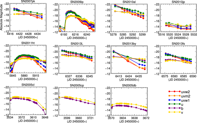
Figure 3. Absolute magnitudes: light curves of our tailored SNe sample and the comparison SNe. This figure does not include SN 2008am and SN 2010jl. The extinction-corrected observed magnitudes were converted to absolute magnitudes using the distances from Table 2. We believe these SNe were observed shortly after maximum UV brightness.
Download figure:
Standard image High-resolution image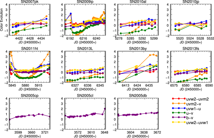
Figure 4. Color evolution for our tailored SNe sample and three comparison SNe. The color–color trends shown are uvw2 – uvm2, uvm2 – v, uvw1 – u, u – v, b – v, and uvw2 – uvw1.
Download figure:
Standard image High-resolution imageOur analysis also includes the blackbody properties of the expanding SN ejecta, i.e., effective temperature, radius, and luminosity. These properties were generated under the assumption that the expanding SN material has blackbody properties. We acknowledge that SN ejecta properties deviate from a blackbody model during later times of the expansion phase, and that the layer underneath the outermost ejecta may be a better approximation to a blackbody. However, this study focuses on analyzing the blackbody properties during the early phases of the expansion when the ejected SN material is still considered to be optically thick. The blackbody properties are used to investigate the relationship between multi-wavelength observations and the basic physical properties of the expansion. The blackbody temperature, radius, and luminosity for each SN are shown in Figure 5.

Figure 5. Blackbody temperature, radius, and luminosity for the UVOT sample starting at observed UV maximum.
Download figure:
Standard image High-resolution imageThe SN blackbody properties were derived using a method introduced in Pritchard et al. (2014) that compares the samples' observed magnitudes to synthetic SN magnitudes. The synthetic magnitudes were generated from a blackbody spectrum ranging from 30,000 to 1000 K. The observed and synthetic magnitudes were compared using a chi-squared minimization technique. The results from the chi-squared minimization determined the best-fit blackbody curves and blackbody temperature for each SN at each epoch. These blackbody temperatures are used to calculate the flux. The radius at each epoch is calculated using the calculated blackbody flux, the flux from observations, and the distances provided in Table 2. This blackbody modeling technique is best at early times when the SN ejecta is considered to be optically thick. As the material expands and cools, it diffuses, becomes optically thin, and deviates from the blackbody model. The luminosities are generated using the blackbody temperatures and the radius. Figure 5 displays the evolution of the blackbody properties for the UVOT sample post maximum brightness. The basic evolution of the properties shows that, as the radius increases, the luminosity and temperature decrease.
In this subsection, we provide a general description of the observational features for each SN, such as UV and optical decay, color evolution, and blackbody trends. For many of these SNe, it is uncertain how long after peak luminosity the SN was observed; therefore, it is unclear where along the SN evolutionary phase these observations occur. These uncertainties hinder a systematic comparison of our sample based on the peak absolute magnitudes. Therefore, the peak magnitudes presented are based on the SN's Swift discovery date. The peak magnitudes will be compared and discussed in Section 3.3.
3.1.1. SN 2005cl
SN 2005cl was discovered by the Lick Observatory Supernova Search (LOSS) on 2005 June 2 and observed in the optical and infrared bands (Kiewe et al. 2012). No UV observations are available; therefore, we only use the optical observations as a comparison. SN 2005cl has been classified as Type IIn according to its spectrum and photometry observations, which reveal a peak absolute magnitude of −18.0 in the v band. The decay slope in the b and v filters is 0.04 and 0.03 mag/day, respectively. There is a rapid decline after 80 days, dropping about 2.5 mag in 20 days. The only color trend available for this SN is b – v and it demonstrates little variation, with a slope of 0.008.
3.1.2. SN 2005cp
SN 2005cp was discovered by LOSS on 2005 June 20 and observed in the optical and infrared (Kiewe et al. 2012). Here we only use the optical for our comparison. The peak absolute v magnitude is −18.5. SN 2005cl has a decay of 0.01 mag/day in the v filter and 0.02 mag/day in the b filter. This SN demonstrates the least change in the b – v color with a slope of 0.003.
3.1.3. SN 2005db
SN 2005db was discovered by Monard on 2005 July 19 (Kiewe et al. 2012). This SN was discovered early enough to detect a slight rise in the light curve. SN 2005db has a peak v magnitude of −15.5 with a decay rate of 0.019 mag/day, and 0.023 mag/day in the b filter. The b – v color evolution has a slope of 0.005.
3.1.4. SN 2007pk
SN 2007pk was reported on November 10.31 UT with an apparent unfiltered magnitude of 17.0. A null image of the SN region was taken five days before discovery on November 5.33 (Parisky & Li 2007). This well-studied SN is typically classified as a SN 1998S-like event, based on its early spectrum. SN 2007pk was first observed by UVOT on November 13.16, about three days after discovery. A peak in the v filter, three days after the first UVOT observation, suggests that this SN was detected within a couple of days after UV maximum (Pritchard et al. 2012). At the time of UVOT discovery, SN 2007pk was extremely UV-bright, with an absolute peak UV magnitude of −20.3, and a fainter optical peak magnitude of −18.2. The UV decay post maximum is steeper than the optical decay, with a 0.2 mag/day UV decay and a 0.04 mag/day optical decay. The uvm2 – v color transitions from blue to red quickly over time with a slope of 0.19. The uvw2 – uvm2 and b – v demostrate the least amount of change, both with a slope of 0.01. From Figure 5, at the time of discovery, SN 2007pk has a maximum blackbody temperature of 19,200 K, a peak blackbody luminosity of 6.3 × 10⁹ L⊙, and the initial radius is 33.5 au.
3.1.5. SN 2009ip
SN 2009ip was first discovered by Maza et al. (2009) on 2009 August 21.14 with an unfiltered magnitude of 19.0. In 2009, it was classified as a faint IIn based on its spectrum, but it faded from detection shortly after discovery. The 2009 event was later classified as a massive explosion from a LBV. In 2012, this SN rebrightened and was discovered with an observed v magnitude of 16.8 (Drake et al. 2012; Prieto et al. 2012; Margutti et al. 2013). UVOT observations of SN 2009ip were made early enough to detect the rise in the light curve. The light curves reveal a steep initial rise, across all six UVOT filters, leading to maximum luminosity. SN 2009ip is UV-bright at maximum luminosity with a peak absolute magnitude of −19.5 in the UV filter and an optical peak, two magnitudes fainter, of −17.8. This SN has a temporal UV decay of 0.14 mag/day and an optical decay of 0.07 mag/day. The color evolution after peak magntiude transistions from blue to red. For this SN, the uvm2 – v color trend demonstrates the most change with a slope of 0.083. The color that demonstrates the least amount of change is the uvw2 – uvm2 trend with a slope of 0.005. The maximum blackbody temperature for SN 2009ip is 16,500 K, with an initial radius of 31.3 au and a maximum luminosity of 2.9 × 10⁹ L⊙.
3.1.6. SN 2010al
SN 2010al was first discovered on 2010 March 13.03 with an apparent unfiltered magnitude of 17.8. A null image was taken 2010 February 7.12 with a limiting magnitude of 18.8 (Rich 2010). The first UVOT observation was on 2010 March 23.18, ten days after it was initially discovered. During the time of UVOT detection, SN 2010al has a peak absolute UV magnitude of −21.5 and a peak absolute magnitude of −19.3 in the optical. This SN has a steep UV decay, but a rapid decay is observed across all the filters. The temporal UV decay is 0.209 mag/day and the optical decay is 0.084 mag/day. When compared to the rest of its color evolution, the uvm2 – v color trend of SN 2010al demonstrates the fastest change with a slope of 0.16, while the b – v demonstrates the least amount of variation for this SN with a slope of 0.006. At the time of UVOT discovery, SN 2010al had a maximum blackbody temperature of 19,900 K, a maximum luminosity of 19.9 × 10⁹ L⊙, and an initial radius of 56.3 au.
3.1.7. SN 2010jp
SN 2010jp was discovered on 2010 November 11.32 at maximum based on its apparent unfiltered magnitude of 17.2 (Maza et al. 2010; Smith et al. 2012). Null images taken 2010 October 13.32 and 2010 October 22.23 provide upper limit magitudes of 18.5 and 18.0, respectively. SN 2010jp was first observed by UVOT on 2010 November 17.17, about six days after it was first discovered. At the time of the first UVOT observation, this SN has a peak UV magnitude of −16.5 and an optical peak of −15.5. The temporal decay in the UV is 0.06 mag/day and the optical decay is 0.05 mag/day. The uvm2 – v color demonstrates the greatest change and has a slope of 0.08, while the uvw2 – uvm2 slope is 0.001. The maximum blackbody temperature is 12,520 K, the maximum luminosity is 0.13 × 10⁹ L⊙, and the initial radius is 11.5 au. This SN has a slower UV decay rate and a lower UV luminosity than the rest of the sample, which indicates that it was observed later than the rest of the SNe in this sample. The initial discovery observations of SN 2010jp were at peak magnitude in the r filter, suggesting that this SN was observed shortly after UV maximum, but probably much later than the rest of the SNe in our sample because the rapid UV decay is not observed.
3.1.8. SN 2011ht
SN 2011ht was first detected on 2011 September 29.182 UT with an unfiltered magnitude of 17.0 (Boles et al. 2011). Upon the initial discovery, this SN was classified as a supernova imposter. This peculiar event demonstrates characteristics of both a true supernova and a supernova impostor (Humphreys et al. 2012; Roming et al. 2012). The first UVOT observation was on 2011 October 04.08 UT. SN 2011ht is another SN in this sample observed pre-maximum, where the initial rise is quick and is followed by a slow rise to the peak magnitude (Roming et al. 2012). The peak absolute magnitude is −18.3 in the UV and the optical peak is −17.2. SN 2011ht exhibits a slight plateau region, in all six filters, which lasts about 20 days past maximum. In the literature, this feature has been examined and compared to previously studied IIn with the same characteristics. Mauerhan et al. (2013) has compared SN 2011ht to SN 1994W and SN 2009kn, and suggests a new subclass, Type IIn-P. When compared to SN 1994W and SN 2009kn, SN 2011ht exhibits not only similar photometric properties but also similar spectral properties. The rate of decline after the peak magnitude varies from the rest of the sample. The slope post-plateau has a UV decay rate of 0.105 mag/day and a optical decay of 0.04 mag/day. The slope including the plateau region, starting at peak, is 0.09 in the UV and 0.02 in the optical. The uvm2 – v color trend increases at a rate of 0.076 and the uvw2 – uvm2 shows little variation with a slope of 0.008. SN 2011ht has a maximum blackbody temperature of 12,500 K, the blackbody luminosity is 1.2 × 10⁹ L⊙, and its initial radius is 34.3 au.
3.1.9. SN 2013L
SN 2013L was discovered on 2013 January 22.025 UT with a unfiltered apparent magnitude of 15.6 (Monard et al. 2013). SN 2013L was first detected by UVOT on 2013 January 29.00 UT and has a peak absolute magnitude of −20.4 in the UV and −18.7 in the optical. The UV slope is 0.130 mag/day and the optical decay is 0.70 mag/day. The uvm2 – v color has a slope of 0.06 and the color that changes the least for this SN is b – v, with a slope of 0.006. At the time of the first observation, the maximum blackbody temperature is 15,000 K, the maximum blackbody luminosity is 6.4 L⊙, and the initial radius is 55.3 au.
3.1.10. SN 2013by
SN 2013by was first detected on 2013 April 23.54 UT with an unfiltered apparent magnitude of 13.5 (Parker et al. 2013). SN 2013by was first observed with UVOT on 2013 April 24.20 UT, and has absolute peak magnitudes of −20.2 and −18.2 in the UV and optical, respectively. The UV decay is 0.19 mag/day and the optical decay is 0.04 mag/day. The uvm2 – v color reddens at a rate of 0.17. The uvw2 – uvm2 color changes the least for this SN, with a rate of 0.001. It has a maximum blackbody temperature of 20,000 K, a maximum blackbody luminosity of 6.1 × 10⁹ L⊙, and a radius of 22 au.
3.1.11. SN 2013fs
SN 2013fs was discovered on 2013 October 06.73 UT with an apparent magnitude of 16.5 (Nakano et al. 2013). SN 2013fs was first observed by UVOT on 2013 October 09.23 with a UV peak absolute magnitude of −19.4 and the optical peak magnitude is −17.0. The UV decay rate is 0.3 mag/day and the optical decay rate is 0.119 mag/day. The uvm2 – vincreases at a rate of 0.19, while the uvw2 – uvm2 shows little variation with a slope of 0.003. This SN has a maximum blackbody temperature of 24,200 K, a maximum luminosity of 3.1 × 10⁹ L⊙, and an initial blackbody radius of 14.9 au.
3.2. Comparison by Color Evolution
The color evolution for each SN in Figure 4 exhibits a linear reddening in most cases. In order to further analyze the sample's color evolution, the SNe are compared by color index in Figure 6. Since the majority of the SNe were observed some time after maximum, the SNe with unknown maximum dates are normalized to the first epoch. The two SNe with observed maximum magnitudes are normalized to their maximum magnitude epoch. By applying this normalization, we are not suggesting that the first observations are at maximum light, but this normalization provides a baseline for comparing the SNe by color trend. The black solid line in Figure 6 signifies the average color trend for the first 20 days since observed maximum brightness and the gray shaded area encloses the 1σ deviation from the mean. The calculations of average and standard deviation are limited by the SN with the shortest observation time, SN 2010jp. Therefore, without interpolating data the mean and σ values are restricted to 20 days after observed maximum.
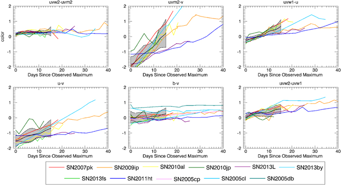
Figure 6. UVOT-observed SNe and comparison SNe compared by color–color. The sample is compared for the first 40 days since observed maximum. SN 2009ip and SN 2011ht are the only two SNe observed before maximum, therefore the rest of the sample was normalized to their first observation. The black line resembles the average color trend and the gray shaded area is the 1σ standard deviation from the average. The comparison SNe appear only in the b – v trend.
Download figure:
Standard image High-resolution imageAs a whole, the sample displays a flat uvw2 – uvm2 color evolution in Figure 6, with little variation from the sample's average. The uvm2 – v color evolves from blue to red, with a large deviation from the mean relative to the uvw2 – uvm2 evolution. The uvm2 – v color trend demonstrates how each SN event decays rapidily at UV wavelengths relative to optical wavelengths. As UV brightness rapidly decays, UV intensities are eventually equivalent to optical intensity at uvm2 – v = 0. A notable feature of this sample is the distinction between the uvm2 – v color trends of the two SNe observed pre-maximum, SN 2009ip and SN 2011ht. The uvm2 – v trend of SN 2011ht demonstrates a flatter shape for the first 10 days after UV peak magnitude, while SN 2009ip displays a linear color evolution starting at peak magnitude.
Normalizing the SN observed after maximum to the first epoch is our chosen baseline, but it is also arbitrary and inconsistent throughout the sample. For each SN observed post maximum, the first observation occurs during an ambiguous phase in the evolution of the explosion, which could vary throughout the sample, making it an unreliable normalization point. The averages presented in Figure 6 were generated with the SNe epochs normalized to the first observation. It is unclear whether a correlation exists between the sample's first observations; therefore, the averages determined based on this normalization method are associated with this systemic error. In order to further investigate and properly compare these SNe based on observational features, a systematic normalization technique is needed. We introduce a method for estimating the date of peak UV magnitude of these SNe, without interpolating data.
3.2.1. Normalizing Method
The first normalization technique attempted used the shock breakout date as the normalization point. Based on the lack of well-constrained shock breakout dates in our sample, the number of days between the estimated shock breakout date and the date of the first UVOT observation is arbitrary and dependent on the error associated with the shock breakout date. Our sample demonstrates the possibility of two different trends in the rise to peak, which introduces an additional uncertainty when trying to establish the number of days since shock breakout. This particular normalization method lacked the desired consistency for comparing the properties of our sample's light curves.
Since the majority of our SNe were observed shortly after peak UV magnitude, we developed a method to estimate the UV maximum date appropriate for our sample, and we use the estimated UV maximum date as a normalization point. Instead of using the number of days between shock breakout and the date of the first UVOT observation as a metric, we identify a common point in the sample's color and blackbody temperature relationship as a reference. Similar to using U – V in UBV photometry for analyzing stars with high temperatures, our method uses a relationship between color and temperature as a tool for determining the peak magnitude for each SN in our sample.
We begin by using the intrinsic UV brightness of these SNe and the rapid decline of uvm2 intensity relative to the semi-constant v brightness in order to gauge the temperature profile of the SN. We use an SN with a full light curve in all six filters as reference in order to identifying how long after maximum the SNe were observed. SN 2009ip is chosen as the reference SN based on the uvm2 – v trend shown in Figure 6, where the majority of the SNe display a similar uvm2 – v behavior to SN 2009ip as opposed to SN 2011ht.
3.2.2. Color and Temperature
The relationship between SN temperatures and uvm2 – v is presented in Figure 7. The temperatures shown in this figure were generated using the technique described in Section 3.1. By analyzing the SN blackbody temperatures as a function of their corresponding uvm2 – v, we can identify a reference point in the sample's temperature and color relationship. Each SN crosses uvm2 – v ∼ −0.9 at some point along its color evolution, and SN 2009ip reaches a temperature of T ∼ 12,000 K at this particular reference point.
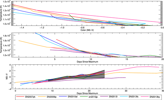
Figure 7. The relationship between color evolution and temperature for UVOT-observed SNe, excluding SN 2011ht. The temperature at each epoch is the result of a best-fit blackbody curve for each epoch. Top panel: temperature as a function of color (uvm2 – v). Using this plot, we find that all the SNe cross T = 12,000 K at uvm2 – v ≈ −0.9. Middle panel: blackbody temperature trends are normalized to the point where they cross T = 12,000 K relative to when SN 2009ip crosses T = 12,000 K. Bottom panel: uvm2 – v is renormalized and a new average and standard are calculated.
Download figure:
Standard image High-resolution imageWe use the known UV maximum date of SN 2009ip to estimate how long after peak UV maximum it takes SN 2009ip to reach T ∼ 12000 K, which we approximate to eight days after peak UV maximum. Then, we determine how long after the first observation it took each of the SNe with unknown UV maximum dates to reach T ∼ 12,000 K. The difference between how long it took SN 2009ip to reach T ∼ 12,000 K (8 days) after UV maximum, and how long after the first observation it took the SN to reach T ∼ 12,000 K is used to estimate how long after peak UV maximum the SN was first observed.
For example, SN 2007pk reaches T ∼ 12,000 K three days after its first UVOT observation. By applying our method, the UV maximum date of SN 2007pk is estimated to be five days before the first UVOT observation. Approximating the UV maximum date with this method introduces the assumption that SNe IIn have a similiar cooling process and will reach the same temperature at the same time after maximum, and in particular the same as SN 2009ip. This cooling feature is not particularly associated with SNe IIn, but an observational feature that this sample does share is the transition from being UV-bright to optically bright at uvm2 – v = 0. Since uvm2 – v = 0 corresponds to T ∼ 10,000 K where our blackbody models introduce uncertainties, we selected a common uvm2 – v value at a higher temperature.
3.2.3. Estimated UV Maximum Date
The SNe discovered post maximum were observed by UVOT as early as one day to as late as 11 days after the initial discovery. SN 2010al was observed by UVOT approximately 11 days after discovery, and has a large error associated with its shock breakout date. The unfiltered magnitudes obtained at the time of discovery were taken three days apart and show a slight increase in magnitude; therefore, it is possible that SN 2010al had not reached maximum luminosity. According to our estimated UV maximum date for SN 2010al, it reached maximum UV brightness 10 days after the first unfiltered observation or approximately one day before the first UVOT observation. Our UVOT observations support the idea that this SN was observed by UVOT shortly after maximum based on its extremely bright UV magnitude and its rapid light curve decay.
In order to verify our estimated maximum dates, we reference previously well-studied SNe in our sample. SN 2007pk has a well-constrained shock breakout date with a 1σ error of 2.5 days. We approximate the UV maximum date to be five days before the first UVOT observation. The estimated UV maximum and shock breakout dates for SN 2007pk suggest a rapid initial rise occurring over a timescale of 1–3 days. SN 2010jp is another well-studied SN included in our sample. This SN was first observed by UVOT approximately six days after its initial discovery. The early observations taken of this region by Maza et al. (2010), before it was officially reported, show an increase in unfiltered magnitudes. SN 2010jp was observed at maximum unfiltered magnitude on the day it was officially reported, which is one day after our estimated UV maximum date (Smith et al. 2012). This supports our approximation since IIn observations have demonstrated that UV intensities tend to peak earlier than optical ones. We were unable to find literary references on the SNe discovered in 2013, but with Swift's rapid response they were observed as early as one day after discovery (SN 2013by and SN 2013fs) and as late as seven days (SN 2013L).
3.2.4. Renormalized uvm2 – v
The bottom panel in Figure 7 shows the uvm2 – v color evolution replotted and normalized. For all the SNe observed after shock breakout, the first observation is normalized to the estimated UV maximum date. The black line is the sample's average uvm2 – v color from day 8 to day 28 and the gray shaded region is one standard deviation from the mean. This renormalized version of the color evolution has less variability from the mean than the uvm2 – v plot in Figure 6. Aside from being the result of a different normalization technique, the mean and standard deviation calculated in Figure 7 do not incorporate SN 2011ht, which was demonstrated to have a distinct uvm2 – v color evolution when compared to the other SNe. SN 2013L evolves more slowly than the rest of the SNe, but its UV light curve also indicates that this SN has a slower UV decay than the rest of the sample. This normalization technique along with our estimated UV maximum dates will be used to compare and analyze our observations.
3.3. Comparison of Absolute Magnitude by Filter
Figure 3 presents the absolute magnitudes in six UVOT filters by SN, while Figure 8 compares the SN by filter. Each light curve is normalized to the number of days from maximum absolute magnitude, using the estimated values defined in the previous section. As previously stated, the majority of the sample is extremely UV-bright and displays a rapid linear decay across all UV filters. Figure 8 provides a general representation of various peak absolute magnitudes, and the sample's decay rates. Overall, the maximum absolute magnitudes and decay rates decrease as wavelength increases. When analyzing by filter, the SN sample seems to follow the same general decay, with the exception of SN 2011ht. The two SNe observed before maximum, SN 2009ip and SN 2011ht, promote the non-uniformity of this subclass by exhibiting different rise and decay trends across all the filters. When the sample is compared to these two SNe, the majority exhibit linear decays similar to SN 2009ip rather than SN 2011ht.
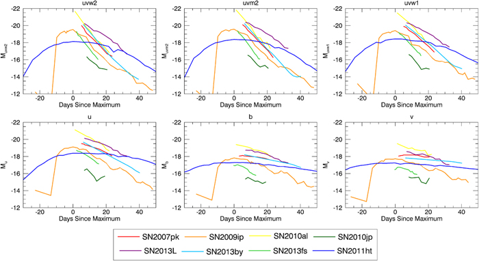
Figure 8. The absolute magnitudes of the UVOT-observed SNe are compared by filter. The time axis is determined by the number of days since maximum determined in Section 3.2.
Download figure:
Standard image High-resolution imageIn Figure 9, the absolute magnitudes are normalized to eight days after maximum brightness, which represents the day on which the color and temperature of SN 2009ip are uvm2 – v ∼ −0.9 and  . This additional normalization provides a reference point along the light curve, which allows us to compare the UV–optical decay rate of each SN. The black line represents the average decay starting at day 8 and the gray shaded region encompasses the 1σ deviation from the mean. When analyzing by filter, the majority of SNe are within one standard deviation from the average. In the UV and U filters, SN 2011ht has a slower decay than the sample and falls outside the 1σ standard deviation. SN 2013L falls slighty outside the standard deviation in the shorter wavelengths, but as the wavelength increases into the near-ultraviolet its trend begins to approach the average decay. In the optical bands, the decay rates are not as fast as the UV decays and display more consistency as they deviate less from the mean. The decay rates slow down considerably in the v filter, and SN 2013by starts to follow a similar decay to SN 2011ht.
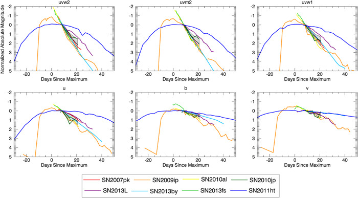
Figure 9. The absolute magnitudes of the UVOT-observed SNe are compared by filter. The sample is normalized to eight days after maximum. The black line signifies the mean decay of the sample, not including SN 2011ht, and the gray shaded area is one standard deviation from the mean.
Download figure:
Standard image High-resolution image3.4. Comparison by Radius, Luminosity, and Temperature
Our observations indicate a variety of peak UV magnitudes and two different UV decay rates. In order to understand our sample's UV behavior, we continue to analyze the blackbody properties of the expanding SN material, with the addition of the expansion velocity and cooling rate. As described in Section 3.1, the temperature, radius, and luminosity of the expanding SN ejecta were calculated for each SN using a blackbody model. The velocity of the expansion during the expanision phase is determined using the change in radius over time. Applying the normalization used in Section 3.2, Figure 10 presents the blackbody properties of the SNe. We study only the first 20 days for each blackbody property since our models underestimate the blackbody temperature as the ejecta expands and cools. This error ultimately affects how the blackbody radius and luminosity are generated at later times. In general, the group increases in radius and decreases in luminosity and temperature, which are characteristics of the SN material as it expands into the CSM. Since the first observations of our SNe occur during different times of the SN evolution, in Table 6 we list the estimated days since UV maximum for each SN in order to compare the SNe blackbody properties.

Figure 10. UVOT sample compared by blackbody (BB) radius, BB luminosity, and BB temperature. The time axis is determined using the days since maximum brightness generated in Section 3.2 and normalized to eight days after maximum.
Download figure:
Standard image High-resolution imageTable 6. Initial BB Radius, Maximum BB Luminosity, and Maximum BB Temperature
| Name | Estimated Days | BB Radius | BB Luminosity | BB Temperture |
|---|---|---|---|---|
| Since UV Max. | (au) | (109 L⊙) | (103 K) | |
| SN 2007pk | 5.2 | 33.5 | 6.3 | 19.2 ± 1.8 |
| SN 2009ip | 0.0 | 31.3 | 3.0 | 16.5 ± 1.4 |
| SN 2010al | 1.3 | 56.3 | 17.0 | 21.2 ± 3.6 |
| SN 2010jp | 8.2 | 11.5 | 0.1 | 12.5 ± 1.5 |
| SN 2011ht | 0.0 | 34.3 | 1.2 | 12.5 ± 0.9 |
| SN 2013L | 7.0 | 55.3 | 6.4 | 15.0 ± 1.5 |
| SN 2013by | 6.3 | 29.3 | 5.6 | 20.0 ± 2.6 |
| SN 2013fs | 2.2 | 14.9 | 3.1 | 24.2 ± 5.5 |
Download table as: ASCIITypeset image
The estimated days since maximum suggests that only five out of the eight SNe were observed relatively close to maximum brightness. These five SNe (i.e., SN 2007pk, SN 2009ip, SN 2010al, SN 2011ht, and SN 2013fs) were observed less than five days from maximum. Out of these five, the brightest SN is SN 2010al, observed approximately one day after maxiumum, and the faintest is SN 2011ht, at maximum luminosity. The hottest SN is SN 2013fs, observed approximately two days after UV maximum, and the SN with the lowest temperature is SN 2011ht at maximum.
As the expansion occurs, the effective temperature begins to drop, and this change in temperature over time for each SN is listed in Table 7. According to the values presented in this table and Figure 10, there seem to be three basic groups depending on cooling rate: the SNe with a rapid cooling rate, the intermediate group, and the group in which the temperature drops gradually over time. SN 2011ht drops in temperature much more slowly than the rest of the SNe, and SN 2013fs cools the fastest, with a cooling rate faster than one standard deviation from the sample average.
Table 7. Change in Temperature and Radius for the First 20 Days
| Name | Expansion Velocity (km s−1) | Cooling Rate (K/day) |
|---|---|---|
| SN 2007pk | 9270 ± 150 | 1020 ± 70 |
| SN 2009ip | 2100 ± 300 | 480 ± 80 |
| SN 2010al | 8130 ± 820 | 1020 ± 100 |
| SN 2010jp | 1140 ± 640 | 470 ± 30 |
| SN 2011ht | 650 ± 60 | 80 ± 20 |
| SN 2013L | 1540 ± 210 | 340 ± 30 |
| SN 2013by | 7000 ± 100 | 820 ± 100 |
| SN 2013fs | 2400 ± 360 | 1120 ± 120 |
| Average | 4030 ± 330 | 670 ± 70 |
Download table as: ASCIITypeset image
The expansion phase is a product of the shock wave induced by the explosion, which accelerates the SN material outward from the center of the massive star. This SN sample's radii expand at two different rates. Table 7 lists the expansion velocities and the associated 1σ uncertainty for each SN and the overall average of the sample. The linear increase of the radii for the first 20 days is used to identify the slope of the trend, or the velocity of the expansion. One group of SNe displays a rapid increase in radius, by an average of 4 au per day, while the other group shows very little change in radius, increasing on average by 0.5 au per day. The average radius of the sample is increasing at a rate of ∼2 au per day. In the first 20 days, SN 2007pk has the fastest expansion velocity and SN 2011ht has the slowest. The expansion velocities of SN 2007pk, SN 2009ip, and SN 2011ht have been estimated spectroscopically. SN 2007pk has an expansion velocity of 8000 km s−1 (Pritchard et al. 2012), SN 2009ip has an ejecta expansion velocity of 2500 km s−1 (Margutti et al. 2013), and the expansion velocity of SN 2011ht has been estimated to be 550 km s−1 by Humphreys et al. (2012) and 646 km s−1 by Roming et al. (2012).
From the expansion and the cooling rate, we can deduce details about the dynamics of the explosion and the properties of the CSM. A SN event with a rapid expansion and cooling rate could be the result of a more energetic explosion, quickly pushing the SN material outward into a relatively less dense, cooler environment. The luminosity is affected by the explosion-driven material interacting with the surrounding CSM, where a circumstellar environment with a diffused density profile interacting with a faster shock wave could produce a more luminous event.
We analyzed the SN blackbody properties in order to understand our observations from a different perspective. The general effects of an expanding ejecta are demonstrated by the increase in radius, and the decrease in luminosity and temperature. However, based on the variation of peak temperatures and luminosities, cooling rates, and expansion velocities, it is unclear whether our observations are characterized by the properties of the explosion or the conditions of the circumstellar environment. We continue to examine the effects of the explosion properties and the conditions of the progenitor star at the time of explosion on our light curves using a modeling approach.
4. LIGHT CURVE MODELS
To better understand our IIn observations, we modified the simple semi-analytic model used by Bayless et al. (2015). This basic light curve model assumes a homologous outflow, like many light curve models, implementing a one-temperature diffusion algorithm to simulate the radiative transport. We use an explicit diffusion transport scheme, limiting our timesteps to the light-travel time which, in general, ensures that the change in energy of each zone is small across any given timestep. Beyond the photosphere, we assume that photon losses quickly radiate away the energy in the zone using an exponential decay time, until the temperature drops below a critical value beyond which we assume no further radiation is emitted from this region. The energy deposition from 56Ni is assumed to be in situ. In the paper of Bayless et al. (2015), the opacities were assumed to be dominated by electron scattering where the ions were assumed to be completely ionized.
Although this light curve model includes many simplifications limiting its application in producing precision light curves, it runs extremely quickly and we can use it to study the role of initial SN conditions on the light curve. With a suite of models, we can study the role of the ejecta velocity, initial temperature (because there are a number of shocks criss-crossing the star, the temperature before breakout can be quite high), composition, and mass distribution (including the 56Ni yield). In addition, this model is ideally suited to include modules that allow us to study the effect of a range of physics. For this set of models, we have included the effect of recombination by altering the opacity when it drops below a given temperature.
One of the primary pieces of physics missing in these calculations is the effect of shock heating as the supernova travels through the circumstellar medium. Many analyses of SN light curves discuss the role of a forward and reverse shock. However, the circumstellar medium is almost certainly inhomogeneous and shocks will permeate the ejecta. As the photosphere moves into this ejecta, shock heating can drastically alter the temperature and position at the photosphere. Since this paper is focused on analyzing the observations, we defer a comprehensive study of these physics effects and initial conditions to a later paper. Instead we focus on matching specific features, i.e., peak luminsosites and decay rates, of the observed light curves to our suite of models. For this paper, we chose six models that best represent the shape of the light curves of the two SNe observed before maximum, SN 2009ip and SN 2011ht, for comparison.
4.1. Modeling Results
Our broad set of models show the extent of the "uniqueness" problem in supernova light curves. We explored the parameter space, i.e., radius of the star, mass of the ejecta, explosion energy, initial temperature, and the density profile, and compared our modeling results to the blackbody profile of SN 2009ip and SN 2011ht, arriving at six "realistic" SN models that best represent our observations. In Figure 11, we present the luminosities and temperatures for model sets A, B, and C, with an explosion energy of 4 × 1051 erg and ranging in ejecta mass from 5 M⊙ to 20 M⊙. Model A assumes a density profile of ρ ∝  , an initial temperature of 1 × 10⁶ K, and a starting radius of 1 × 1012 cm. Models B and C both assume a density profile of ρ ∝ r−2 and a radius of 1 × 1013 cm. The difference between Model B and Model C is the initial temperature. Model B has an initial temperature of 4 × 10⁵ K, while Model C has an initial temperature of 1 × 10⁶ K. Figure 12 shows model sets D, E, and F, which differ from models set A, B, and C in having an explosion energy of 1 × 1051 erg. We compare the models presented in Figures 11 and 12 to the two SNe with full light curves included in our sample. Depending upon the initial conditions, the luminosity of the SNe can be matched both by a photosphere moving through the hot stellar envelope and by a hot core powered by 56Ni decay.

Figure 11. Comparison of the blackbody temperature of SN 2009ip and SN 2011ht with the blackbody temperature and luminosity from our semi-analytical model. The ejecta mass for these models ranges from 5 M⊙ to 20 M⊙ with an explosion energy = 4 × 1051 erg. Top panel: model set A has a density profile of ρ ∝ r−0.5, an initial temperature of 1 × 10⁶ K, and a starting radius of 1 × 1012 cm. Middle panel: model set B has a density profile of ρ ∝ r−2, an initial temperature of 4 × 10⁵ K, and a radius of 1 × 1013 cm. Bottom panel: model set C has a density profile of ρ ∝ r−2, an initial temperature of 1 × 10⁶ K, and a radius of 1 × 1013 cm.
Download figure:
Standard image High-resolution image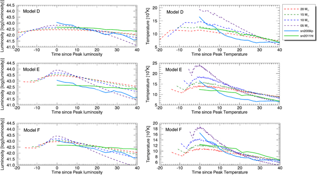
Figure 12. Comparison of the blackbody temperature of SN 2009ip and SN 2011ht with the blackbody temperature and luminosity from our semi-analytical model. The ejecta mass for these models ranges from 5 M⊙ to 20 M⊙ with an explosion energy = 1 × 1051 erg. Top panel: model set D has a density profile of ρ ∝ r−0.5, an initial temperature of 1 × 10⁶ K, and a starting radius of 1 × 1012 cm. Middle panel: model set E has a density profile of ρ ∝ r−2, an initial temperature of 4 × 10⁵ K, and a radius of 1 × 1013 cm. Bottom panel: model set F has a density profile of ρ ∝ r−2, an initial temperature of 1 × 10⁶ K, and a radius of 1 × 1013 cm.
Download figure:
Standard image High-resolution imageModel sets A and D represent the luminosities powered by 56Ni decay, while the rest of the models are the result of the photosphere receding and moving through the stellar material. In both of these cases, the models that matched the luminosity and the temperatures were unable to match the low blackbody radii inferred from the observations. The luminosity and temperature trend of SN 2009ip matches with the trends from Model C, the models with the greater explosion energy and a wind-like density profile, which are powered by the receding photosphere. However, the luminosity and temperature trend of SN 2011ht matches better with the result from Model D, the models with a lower explosion energy and a flatter density profile where the luminosity is produced by 56Ni decay.
We compare the uvm2 light curves of SN 2009ip and SN 2011ht to the modeled uvm2 light curve produced with UVOT response curves. In Figure 13, the uvm2 light curve of SN 2009ip is compared to a modeled uvm2 light curve with an ejecta mass of 20 M⊙ from Model C, while in Figure 14 the uvm2 light curve of SN 2011ht is compared to a modeled uvm2 light curve with an ejecta mass of 15 M⊙ from Model D. By comparing the absolute magnitudes from our observed SNe to the modeled light curves, we see how our models do not match up perfectly with the peak magnitudes, but the modeled decay rate does match the observations. Our modeling results indicate that the peak luminosity is sensitive to the initial condition of the progenitor stellar environment, i.e., mass of the ejecta, explosion energy, initial internal temperature. These models also demonstrate how the luminosity decay and cooling rate depend on the energy of the explosion, the density profile, and the interaction powering the SN luminosity, i.e., 56Ni decay or a receding photosphere.

Figure 13. The uvm2 light curve of SN 2009ip is compared to the uvm2 light curve produced through Model C with an ejecta mass of 20 M⊙. Model set C has a density profile of ρ ∝ r−2, an initial temperature of 1 × 10⁶ K, and a radius of 1 × 1013 cm.
Download figure:
Standard image High-resolution image
Figure 14. The uvm2 light curve of SN 2011ht is compared to the uvm2 light curve produced through Model D with an ejecta mass of 15 M⊙. Model set D has a density profile of ρ ∝ r−0.5, an initial temperature of 1 × 10⁶ K, and a starting radius of 1 × 1012 cm.
Download figure:
Standard image High-resolution image
5. DISCUSSION
Studies of SNe IIn tend to focus around highly luminous events, but our IIn sample is unbiased toward extraordinary events, and the SN selection is completely based on the availability of nearby SNe IIn with early observations. The sample size is small and the majority of our SNe were observed after maximum light, with the exception of two SN events with observations during the rise to peak. In general, the SNe IIn in our sample exhibit a rapid decay in UV magnitude relative to the optical decay rates. The SNe with observed rise to peak exhibit different light curve features, promoting the currently accepted heterogeneous nature of this subclass. At peak magnitude, SN 2009ip is brighter than SN 2011ht and exhibits a sharper rise to the peak. These two SNe have different light curve shapes, with SN 2011ht showing a prolonged maximum period.
IIn events have been labeled as heterogenous based on the properties of optical light curves, but we analyze the UV behavior in order to gain a different perspective. In our study, we demonstrated that, when compared by wavelength, the majority of our sample displays a similar behavior based on their UV decay. If we attempt to classify our SNe sample based entirely on the rate of UV magnitude decay, there seem to be two types of SNe in our sample: UV fast and UV slow. The majority of our sample falls in the group with the fast UV decay, and are comparable to SN 2009ip. Even though decay rates display similar characteristics, our observations show a broad range of peak magnitudes. The SNe included in our sample are brighter in the UV at the time of peak magnitude, and the light curves display a transition phase from being UV-bright to being optically bright.
The difference between the SNe with fast UV decay and slow UV decay could be dependent on the structure of the environment surrounding the star prior to the explosion, along with the dynamics of the explosion. If the SN explosion is weak and the SN ejecta is powered by a slow shock wave, UV radiation would be produced over a sustained period of time as the ejecta slowly interacts with the optically thick shell. This shock breakout scenario would result in a prolonged period of UV emissions and this could be the case for SN 2011ht. On the other hand, if the SN explosion is strong enough to break through the optically thick shell quickly, then the SN ejecta would be accelerated by a faster shock when it interacts with the CSM and as it eventually enters the stellar wind region. This type of explosion environment would display a quick rise to peak, and the decline phase would also drop quickly as the photosphere expands quickly into the stellar wind material. Therefore, a combination of the explosion properties, shell structure, and stellar wind properties will affect the rise and decay phases of the IIn light curves.
The rise to peak UV magnitude for the majority of our SNe was not observed. The initial UV rise occurs very quickly and is very difficult to observe. From the estimated date of UV peak magnitude and upper-limit observations, SN 2007pk might have had an extremely rapid rise, lasting 2–3 days, relative to the two SNe with observed rise times. SN 2009ip demonstrates an initial UV rise of ∼10 days, while SN 2011ht shows an initial rise of ∼15 days. SN 2011ht has a prolonged maximum period of about 20 days, while SN 2009ip begins to decay quickly after UV maximum. These observations indicate a variation of rise times and peak magnitudes, but from this sample it is unclear whether a rapid UV decay coincides with a rapid UV rise.
For an alternative perspective on how these SNe evolve, we analyzed the blackbody properties of the explosion during early times. Overall, the sample increases in radius and decreases in luminosity and temperature as the ejecta expands and cools. During the first 20 days since UV maximum, there are SNe with quickly evolving blackbody properties, and SNe that demonstrate little to no change. SN 2007pk, SN 2010al, and SN 2010fs were observed shortly after peak magnitude and display similar characteristics of their UV light curves, but their different blackbody characteristics suggest that early UV emissions are produced under various photospheric conditions. A correlation between the early behavior of the UV light curve and early blackbody properties was not apparent, therefore our sample could not be characterized using the evolution of the SN blackbody properties. We continued to search for a characteristic feature that connects our observations to the properties of the photospheric boundary. Since the expansion phase is dependent on the dynamics of the explosion and the physical properties of the circumstellar environment, we examined the role of these SN environments on our observations.
We used a simple semi-analytical model in order to understand the relationship between our observations and the properties of the expanding SN ejecta. Scientists have used a broad range of techniques to model supernova light curves and spectra, each with their own set of simplifying assumptions. These methods include back-of-the-envelope estimates that often assume that radioactive decay dominates the light curve, e.g., Soderberg et al. (2006), Kasen & Woosley (2009), detailed transport where radiation–hydrodynamics coupling is neglected, e.g., Mazzali et al. (2015), and full radiation–hydrodynamics models with simplified transport solutions (e.g., Frey et al. 2013; Kozyreva & Blinnikov 2015). Our calculations are sufficiently detailed to capture many of the effects in these more sophisticated models, including the effects of shock heating based on the initial temperature, while running fast enough to do parameter studies. Shock heating occurs both within the star and when the shock breaks out of the star. We include shock heating in our models by assuming an initial temperature of either 4 × 10⁵ K or 1 × 10⁶ K. The models with the lower initial temperature, Model B and Model E, were unable to match the SN luminosities.
Our models demonstrate that, depending upon the initial conditions, the luminosity of SN 2009ip and SN 2011ht can be matched both by a photosphere moving through the hot stellar envelope and by a hot core powered by 56Ni decay, respectively. The fast rise and decay correspond to the models representing a photosphere moving through the envelope, while the modeled light curves with a slower rise and decay rate are powered by 56Ni decay. However, in both of these cases, models that matched the luminosity were unable to match the low radii from the blackbody models. This could be because the model assumes that the ejected supernova material can be explained by a homologous expansion, where the velocity of the ejecta is proportional to its initial radius. Either simplifications in the calculation of blackbody properties are leading to an overestimated modeled photospheric radius or our simulations are still missing some physics.
6. CONCLUSION
We present a sample of eight SNe IIn observed with Swift UVOT. Based on a 1σ standard deviation from the average UV decay rate, six of the SNe display a fast UV decay and two exhibit a slow UV decay. Given our small sample size, it is difficult to determine whether the UV-slow SNe are special cases or whether the deviating SNe are part of a wider spectrum of IIn UV decay rates. IIn are referred to as heterogeneous based on optical peak magnitudes, but instead we compare our SNe based on their UV behavior to understand their true nature. Since comparing maximum luminosities at the time of discovery (for SNe observed post maximum) introduces a systematic error, we estimated the peak magnitude dates using a color–temperature relationship, and standardize our comparison of light curves to the date of peak magnitude.
We generated the blackbody properties of the expanding photosphere, i.e., luminosity, temperature, and radius, in order to further investigate our observations. By analyzing the physical parameters of the photosphere, we arrived at a simple shock breakout scenario that could produce the behavior of the UV light curves we observe during early times. When we compare SNe from our sample to a set of modeled SNe, we begin to see the influence of initial explosion conditions on early properties of UV light curves such as peak luminosities and decay rate. The SNe in our sample have different peak UV magnitudes, which our models indicate could be the result of different progenitor star conditions. Our observations indicate that the peak UV magnitudes of this SN subclass varied considerably, with an average difference of 2 mag. From our semi-analyical model, it was difficult to determine a unique set of explosion conditions that result in these peak magnitudes.
On the other hand, under the limitations of our current model, the shape of the light curve can constrain the density profile of the progenitor. A shallow decay is better fit by a stellar structure with a flatter density, possibly dominated by a giant envelope, whereas the faster decays are better fit by an r−2 profile, arguing that the photosphere is in a wind-like structure prior to collapse. Depending on the stellar evolution, both of these scenarios should exist, and determining the fraction of each scenario will provide a better understanding of the evolution of these massive stars. We plan to continue examining these effects by exploring the rest of the parameter space, redefining the initial modeling conditions to incorporate an outer shell-like structure and to include late-time shock heating from shocks produced as the supernova ejecta travels through the inhomogeneous circumstellar medium. Based on the initial temperatures used in our set of models, we will need to incorporate shock heating as the shock travels through the interior of the star and the stellar wind. The effect of shock heating as the SN material blasts through the CSM can drastically alter the temperature and position of the photosphere. We will study the role of shock heating in IIn light curves in more detail in a subsequent paper.