


ABSTRACT
We performed a comprehensive stacking analysis on ∼14,200 quiescent galaxy (QG) candidates at z = 0–3 across mid-, far-infrared (MIR and FIR), and radio wavelengths. Identified via their rest-frame NUV − r and r − J colors, the QG candidates ( ) have drastically different IR and radio properties depending on their 24 μm emission strength. The fraction of QG candidates with strong 24 μm emission (equivalent to inferred star formation rates SFR
 , hereafter "IR-bright") increases with redshift and peaks at 15%, and their stacked MIPS 24 μm, Herschel (PACS and SPIRE) and VLA emissions are consistent with being star-forming galaxies (SFGs). In contrast, the majority of QG candidates are faint or undetected at 24 μm individually (i.e., SFR24 < 100 M⊙ yr−1, hereafter "IR-faint"). Their low dust-obscured SFRs derived from Herschel stacking (SFRH ≲ 3, 15, 50 M⊙ yr−1 out to z ∼ 1, 2, 3) are >2.5–12.5× lower than compared to SFGs. This is consistent with the quiescence, as expected from their low unobscured SFRs, as inferred from modeling their ultraviolet-to-NIR photometry. The discrepancy between the LIR derived from stacking Herschel and 24 μm indicates that IR-faint QGs have dust SEDs that are different from those of SFGs. For the most massive (
 ) IR-faint QGs at z < 1.5, the stacked 1.4 GHz emission is in excess of that expected from other SFR indicators, suggesting a widespread presence of low-luminosity active galactic nuclei. Our results reaffirm the existence of a significant population of QGs out to z = 3, thus corroborating the need to quench star formation in galaxies at early epochs.
Export citation and abstract BibTeX RIS
1. INTRODUCTION
Studies suggest that when the universe was only 4 Gyr old (z ∼ 1.5), about half of the most massive ( ) galaxies already had evolved stellar populations and unobscured SFRs of only a few M⊙ yr−1 (e.g., Ilbert et al. 2013; Muzzin et al. 2013, and references therein). They are thought to have undergone a rapid build-up of stellar mass followed by an effective phase of star formation quenching, possibly via AGN feedback (e.g., Bower et al. 2006; Croton et al. 2006). However, these claims rest on the assumption of a universal dust attenuation law (Calzetti et al. 2000), which may in fact vary with galaxy spectral types (Kriek & Conroy 2013). If a significant amount of heated dust is present in these galaxies, however, it would imply that the SFRs inferred from the rest-frame ultraviolet (UV) are severely underestimated, and that their red colors are due to strong dust reddening, rather than evolved stellar populations. Direct FIR measurement of the cold dust is essential to unambiguously assess the level of obscured SF. A recent Herschel13
stacking analysis by Viero et al. (2013) found that massive QGs at z > 2 have IR luminosities comparable to local starbursts (i.e., ultra-luminous IR galaxies or ULIRGs,
) galaxies already had evolved stellar populations and unobscured SFRs of only a few M⊙ yr−1 (e.g., Ilbert et al. 2013; Muzzin et al. 2013, and references therein). They are thought to have undergone a rapid build-up of stellar mass followed by an effective phase of star formation quenching, possibly via AGN feedback (e.g., Bower et al. 2006; Croton et al. 2006). However, these claims rest on the assumption of a universal dust attenuation law (Calzetti et al. 2000), which may in fact vary with galaxy spectral types (Kriek & Conroy 2013). If a significant amount of heated dust is present in these galaxies, however, it would imply that the SFRs inferred from the rest-frame ultraviolet (UV) are severely underestimated, and that their red colors are due to strong dust reddening, rather than evolved stellar populations. Direct FIR measurement of the cold dust is essential to unambiguously assess the level of obscured SF. A recent Herschel13
stacking analysis by Viero et al. (2013) found that massive QGs at z > 2 have IR luminosities comparable to local starbursts (i.e., ultra-luminous IR galaxies or ULIRGs,  ), inconsistent with the quiescence inferred from the UV continua (e.g., Ilbert et al. 2013) as well as their low 24 μm stacked flux densities (Fumagalli et al. 2014; Utomo et al. 2014). If QGs harbor significant dust-obscured SF, it would bring into question the usefulness of the rest-frame color selections commonly used for identifying QGs (e.g., Williams et al. 2009; Ilbert et al. 2013), therefore challenging the need for powerful quenching mechanisms.
Here, we analyze a sample of ∼14,200 QG candidates with  out to z = 3, selected over an area of 1.48 deg2 in the COSMOS field (Scoville et al. 2007). The large sample size enables us to use stacking to enhance the sensitivity to study otherwise undetected sources. A comprehensive stacking analysis across MIR, FIR, and radio wavelengths using the same sample is necessary for interpreting the inconsistent dust-obscured SFRs in the literature obtained by stacking 24 μm and Herschel, as mentioned above. Taking advantage of the available deep multi-wavelength data, we constrain their dust-obscured SFRs through stacking in the Spitzer Multiband Imaging Photometer (MIPS; Rieke et al. 2004), the Herschel Photodetector Array Camera, and Spectrometer (PACS; Poglitsch et al. 2010), and the Spectral and Photometric Imaging Receiver (SPIRE14
; Griffin et al. 2010) maps. These are compared with stacks in deep Very Large Array (VLA) radio maps. Magnitudes are quoted in the AB system. We adopt a Chabrier (2003) initial mass function (IMF), and H0 = 70 km s−1 Mpc−1, ΩM = 0.3, and ΩΛ = 0.7. All the infrared luminosities (LIR) used in this work are integrated from the rest-frame wavelength range of 8–1000 μm.
out to z = 3, selected over an area of 1.48 deg2 in the COSMOS field (Scoville et al. 2007). The large sample size enables us to use stacking to enhance the sensitivity to study otherwise undetected sources. A comprehensive stacking analysis across MIR, FIR, and radio wavelengths using the same sample is necessary for interpreting the inconsistent dust-obscured SFRs in the literature obtained by stacking 24 μm and Herschel, as mentioned above. Taking advantage of the available deep multi-wavelength data, we constrain their dust-obscured SFRs through stacking in the Spitzer Multiband Imaging Photometer (MIPS; Rieke et al. 2004), the Herschel Photodetector Array Camera, and Spectrometer (PACS; Poglitsch et al. 2010), and the Spectral and Photometric Imaging Receiver (SPIRE14
; Griffin et al. 2010) maps. These are compared with stacks in deep Very Large Array (VLA) radio maps. Magnitudes are quoted in the AB system. We adopt a Chabrier (2003) initial mass function (IMF), and H0 = 70 km s−1 Mpc−1, ΩM = 0.3, and ΩΛ = 0.7. All the infrared luminosities (LIR) used in this work are integrated from the rest-frame wavelength range of 8–1000 μm.
2. DATA AND SAMPLE SELECTION
We select galaxies brighter than Ks = 24 from the UltraVISTA survey (McCracken et al. 2012) which have  and photometric redshifts zphot = 0.1–3.0. Both M⋆ and zphot are from the catalog of Ilbert et al. (2013), derived from spectral energy distribution (SED) fits to the broadband UV-to-IRAC photometry (Capak et al. 2007). A small fraction of the UltraVISTA galaxies appears to host AGNs (<5%), as indicated via their emission in X-rays (Brusa et al. 2010; Civano et al. 2012), IRAC bands (Donley et al. 2012), or the radio (Schinnerer et al. 2007, 2010). We have included them in the analysis presented below, but we note that excluding them does not change the 24 μm and radio (the two bands expected to be most sensitive to the presence of an AGN) stacked flux densities within the stated uncertainties, nor the conclusions of this work.
Multiple rest-frame color selection techniques have been devised to separate QGs from SFGs, such as U − V versus V − J ("UVJ-selection"; Williams et al. 2009), NUV − r versus r − J ("NUVrJ-selection"; Ilbert et al. 2013), and NUV − r versus r − K (Arnouts et al. 2013). Here, we have adopted the NUVrJ selection technique for the reasons explained in Ilbert et al. (2013, Section 3.3), although we note that the stacking results from our selection are comparable to those using the UVJ-selection (see Section 4.7). Each galaxy is classified as a QG or a SFG candidate15 based on its rest-frame NUV − r and r − J colors, where the criterion is shown on Figure 1. NUV − r is a measure of the amount of UV light from young stars (i.e., recent SF) relative to the red optical light from evolved stellar populations, and when compared to r − J we obtain constraints on the degree of dust attenuation. The QG candidates are divided into six bins of zphot, each of which is split into four M⋆-bins (see Table 2); however, only M⋆-bins which are >90% mass-complete (according to the limits presented in Ilbert et al. 2013) are considered and stacked,16 as listed in Table 2.
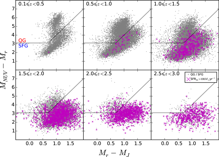
Figure 1. Rest-frame NUV − r and r − J colors for galaxies above the mass-completeness limits (small gray dots) from the UltraVISTA survey (Ilbert et al. 2013). QG candidates are defined as having  and
and  . The QGs/SFGs classification boundary is marked by gray solid lines. Galaxies with SFR
 yr−1 are indicated as magenta crosses, and those within the QG region are considered as "IR-bright QGs" in this paper.
Download figure:
Standard image High-resolution imageTo weed out dusty galaxies erroneously classified as QGs, we cross-correlate our sample, using a radius of  , with the MIPS 24 μm catalog of Le Floc'h et al. (2009), which is 90% complete for sources with
  80 μJy. A redshift-dependent 24 μm flux density (S24) cut-off17
is then applied to separate the IR-bright QG candidates with SFR
80 μJy. A redshift-dependent 24 μm flux density (S24) cut-off17
is then applied to separate the IR-bright QG candidates with SFR yr−1, where SFR24 is the SFR inferred from their 24 μm flux density (S24; see Section 4.4 for derivation). The fraction of QG candidates with SFR
 yr−1 (
 ) increases with z and peaks at 15% for the most massive ones at z ≳ 2 (see Table 1), qualitatively similar to the trend found in Marchesini et al. (2014). This suggests a higher fraction of misclassified QG candidates at z ≳ 2, which results from a higher fraction of dusty galaxies at higher z (e.g., Greve et al. 2010), and more uncertain rest-frame colors (Williams et al. 2009). Overall, however, the fractions are reassuringly small. A similar conclusion is reached for the fraction (
 Table 1) of QG candidates that are further detected by Herschel (i.e., S/N
  in at least two PACS and/or SPIRE bands), determined using the catalog of Lee et al. (2013) in which the 24 μm sources presented in Le Floc'h et al. (2009) are cross-identified to the Herschel detections. The linear inversion technique of cross-identification being used is described in Roseboom et al. (2010, 2012).
Table 1. 24 μm- and Herschel-bright Fractions for QG Candidates
| log(M⋆/M⊙) | ||||
|---|---|---|---|---|
| Redshift | 11–12.2 | 10.6–11 | 10.2–10.6 | 9.8–10.2 |
| fQG, 24 | ||||
| 0.1–0.5 | 0% | 0% | 0% | 0% |
| 0.5–1.0 | 0.2% | 0.1% | 0% | 0% |
| 1.0–1.5 | 2.1% | 0.8% | 0.2% | 0% |
| 1.5–2.0 | 2.4% | 4.7% | 2.6% | ⋯ |
| 2.0–2.5 | 14.7% | 9.9% | ⋯ | ⋯ |
| 2.5–3.0 | 13.3% | ⋯ | ⋯ | ⋯ |

|
||||
| 0.1–0.5 | 0% | 0% | 0% | 0% |
| 0.5–1.0 | 0.2% | 0.1% | 0% | 0% |
| 1.0–1.5 | 0.8% | 0.1% | 0% | 0% |
| 1.5–2.0 | 1.2% | 1.0% | 0.6% | ⋯ |
| 2.0–2.5 | 6.0% | 2.5% | ⋯ | ⋯ |
| 2.5–3.0 | 2.7% | ⋯ | ⋯ | ⋯ |
Note.  is the fraction of QG candidates (classified by their NUV − r and r − J colors) with SFR24 ≥ 100 M⊙ yr−1, where SFR24 is the SFR as inferred from the 24 μm flux density.
  is the fraction of QG canididates fulfilling the above criterion that are also detected in at least two Herschel PACS+SPIRE bands (S/N ≥ 5).
Download table as: ASCIITypeset image
For the stacking analysis (Section 3) we use the MIPS 24 μm imaging (FWHM ≃ 6'') from Sanders et al. (2007), while the Herschel PACS and SPIRE maps are from the PACS Evolutionary Probe survey (PEP; Lutz et al. 2011) and the Herschel Multi-tiered Extragalactic Survey (HerMES; Oliver et al. 2012), respectively. The PACS maps reach depths of 5 and 10.3 mJy beam−1 (3σ) at 100 and 160 μm, respectively (FWHM ≃ 6 8 and 11''), and SPIRE 250, 350, and 500 μm depths are 8, 11, and 13 mJy beam−1 (3σ), respectively (FWHM ≃ 182, 249, and 363). The Herschel maps are made assuming a flat spectrum. For the radio stacking we use the 1.4 GHz VLA-COSMOS large survey (Schinnerer et al. 2007, 2010), which reaches a root-mean-square noise (rms) of 15 μJy beam−1 at an angular resolution of ∼15 (FWHM).
3. STACKING
Our Herschel maps are characterized by a high level of source confusion (multiple sources blended in a beam due to coarse angular resolution; Nguyen et al. 2010) which, if unaccounted for, will bias a stacked signal of clustered sources (Marsden et al. 2009; Béthermin et al. 2010; Kurczynski & Gawiser 2010; Viero et al. 2013). Here, we apply the global stacking and deblending method presented in Viero et al. (2013), which is publicly distributed as an IDL code called SIMSTACK.18 In short, we stacked and deblended multiple galaxy samples simultaneously, including a separate list of 24 μm sources from Le Floc'h et al. (2009) that are not already included in the UltraVISTA sample. The median M⋆ and z for IR-faint QGs, IR-bright QGs, and SFGs are listed in Tables 2–4, respectively. We estimated the errors of the Herschel stacking following the extended bootstrap technique presented in Viero et al. (2013, Section 3.4). Having created 100 fake UltraVISTA catalogs by perturbing M⋆ and z of all sources within their uncertainties, we re-did the sample selection and re-ran SIMSTACK 100 times. The stacked flux densities and errors are taken to be the mean and standard deviation of the 100 runs.
Table 2. Stacked Flux Densities of Spitzer/MIPS 24 μm, Herschel (PACS+SPIRE), and VLA 1.4 GHz and the Inferred SFRs for IR-faint QG Candidates
| Redshift |

|
Ngal | S24 μm | S100 μm | S160 μm | S250 μm | S350 μm | S500 μm | Sradio | log( ) ) |
log( ) ) |
qIR | SFRSED | SFR24 | SFRH | SFRradio | log(sSFRH) |
|---|---|---|---|---|---|---|---|---|---|---|---|---|---|---|---|---|---|
| (μJy) | (mJy) | (mJy) | (mJy) | (mJy) | (mJy) | (μJy) | log(L⊙) | log(W Hz−1) | (M⊙ yr−1) | (M⊙ yr−1) | (M⊙ yr−1) | (M⊙ yr−1) | log(yr−1) | ||||
| log(M⋆/M⊙) = 11–12.2 (median = 11.2) | |||||||||||||||||
| 0.1–0.5 | 0.4 | 232 | 34.0 ± 1.5 | 0.5 ± 0.1 | 2.0 ± 0.2 | 0.6 ± 0.3 | 1.9 ± 0.2 | 1.1 ± 0.2 | 9.6 ± 1.1 | 9.8 ± 0.1 | 21.7 ± 0.0 | 2.2 |

|
0.5 ± 0.2 |

|
1.7 ± 0.1 | −11.3 |
| 0.5–1.0 | 0.8 | 1298 | 24.1 ± 0.9 | 0.1 ± 0.0 | 1.2 ± 0.1 | 0.6 ± 0.1 | 2.3 ± 0.1 | 1.2 ± 0.1 | 7.8 ± 0.5 | 10.5 ± 0.1 | 22.5 ± 0.0 | 2.1 |

|
1.8 ± 0.7 |

|
9.2 ± 0.5 | −10.6 |
| 1.0–1.5 | 1.2 | 827 | 21.3 ± 1.0 | 0.2 ± 0.0 | 1.0 ± 0.1 | 0.7 ± 0.2 | 2.5 ± 0.1 | 1.4 ± 0.1 | 6.4 ± 0.6 | 10.9 ± 0.1 | 22.8 ± 0.0 | 2.1 |

|
4.6 ± 1.7 |

|
19.0 ± 1.7 | −10.2 |
| 1.5–2.0 | 1.6 | 320 | 13.0 ± 1.2 | 0.0 ± 0.1 | 0.6 ± 0.2 | −0.1 ± 0.3 | 2.4 ± 0.3 | 2.0 ± 0.2 | 3.0 ± 0.9 | 11.2 ± 0.2 | 22.8 ± 0.1 | 2.4 |

|
4.8 ± 1.8 |

|
20.0 ± 6.0 | −10.0 |
| 2.0–2.5 | 2.2 | 185 | 17.6 ± 1.6 | −0.1 ± 0.1 | 1.3 ± 0.3 | 0.6 ± 0.4 | 3.1 ± 0.4 | 2.5 ± 0.3 | 5.7 ± 1.1 | 11.7 ± 0.1 | 23.4 ± 0.1 | 2.3 |

|
9.4 ± 3.5 |

|
82.7 ± 16.6 | −9.4 |
| 2.5–3.0 | 2.6 | 65 | 11.7 ± 2.2 | −0.2 ± 0.1 | 0.4 ± 0.5 | −1.2 ± 0.6 | 1.4 ± 0.6 | 1.7 ± 0.6 | 6.0 ± 2.1 | 11.5 ± 0.4 | 23.6 ± 0.1 | 1.9 |

|
12.8 ± 5.4 |

|
141.2 ± 48.4 | −9.5 |
| log(M⋆/M⊙) = 10.6–11.0 (median = 10.8) | |||||||||||||||||
| 0.1–0.5 | 0.4 | 518 | 26.3 ± 1.0 | 0.7 ± 0.1 | 2.5 ± 0.2 | 0.4 ± 0.2 | 1.8 ± 0.2 | 1.0 ± 0.2 | 4.8 ± 0.7 | 9.9 ± 0.1 | 21.4 ± 0.1 | 2.5 |

|
0.3 ± 0.1 |

|
0.9 ± 0.1 | −10.9 |
| 0.5–1.0 | 0.8 | 2296 | 16.5 ± 0.7 | 0.2 ± 0.0 | 1.2 ± 0.1 | −0.1 ± 0.1 | 1.9 ± 0.1 | 1.3 ± 0.1 | 2.9 ± 0.3 | 10.5 ± 0.0 | 22.0 ± 0.1 | 2.5 |

|
1.2 ± 0.4 |

|
3.3 ± 0.4 | −10.3 |
| 1.0–1.5 | 1.2 | 1764 | 10.7 ± 0.5 | 0.1 ± 0.0 | 0.7 ± 0.1 | −0.9 ± 0.1 | 1.6 ± 0.1 | 0.9 ± 0.1 | 2.3 ± 0.4 | 10.8 ± 0.1 | 22.3 ± 0.1 | 2.4 |

|
2.0 ± 0.7 |

|
6.8 ± 1.1 | −10.0 |
| 1.5–2.0 | 1.7 | 550 | 8.5 ± 0.8 | −0.1 ± 0.1 | 0.4 ± 0.2 | −1.5 ± 0.3 | 1.3 ± 0.2 | 1.1 ± 0.2 | 2.8 ± 0.7 | 11.0 ± 0.2 | 22.8 ± 0.1 | 2.2 |

|
2.8 ± 1.1 |

|
20.2 ± 4.8 | −9.8 |
| 2.0–2.5 | 2.2 | 326 | 13.2 ± 1.2 | 0.1 ± 0.1 | 0.8 ± 0.3 | −0.6 ± 0.4 | 2.6 ± 0.4 | 2.1 ± 0.3 | 3.0 ± 0.9 | 11.6 ± 0.2 | 23.2 ± 0.1 | 2.4 |

|
7.5 ± 2.8 |

|
45.6 ± 13.4 | −9.2 |
| log(M⋆/M⊙) = 10.2–10.6 (median = 10.4) | |||||||||||||||||
| 0.1–0.5 | 0.4 | 708 | 13.7 ± 0.8 | 0.5 ± 0.1 | 1.9 ± 0.2 | −1.0 ± 0.1 | 0.7 ± 0.1 | 0.2 ± 0.1 | 3.5 ± 0.6 | 9.7 ± 0.1 | 21.2 ± 0.1 | 2.5 |

|
0.2 ± 0.1 |

|
0.8 ± 0.1 | −10.7 |
| 0.5–1.0 | 0.8 | 2365 | 12.1 ± 0.5 | 0.2 ± 0.0 | 1.0 ± 0.1 | −1.0 ± 0.1 | 1.1 ± 0.1 | 0.6 ± 0.1 | 1.5 ± 0.3 | 10.3 ± 0.1 | 21.7 ± 0.1 | 2.6 |

|
0.8 ± 0.3 |

|
1.8 ± 0.3 | −10.1 |
| 1.0–1.5 | 1.2 | 1268 | 6.4 ± 0.5 | 0.0 ± 0.0 | 0.7 ± 0.1 | −1.7 ± 0.1 | 1.1 ± 0.1 | 0.9 ± 0.1 | 1.5 ± 0.5 | 10.7 ± 0.1 | 22.1 ± 0.1 | 2.6 |

|
1.1 ± 0.4 |

|
4.3 ± 1.3 | −9.7 |
| 1.5–2.0 | 1.7 | 478 | 7.0 ± 0.9 | 0.0 ± 0.1 | 0.7 ± 0.2 | −1.6 ± 0.3 | 1.3 ± 0.3 | 1.1 ± 0.2 | 2.0 ± 0.7 | 11.1 ± 0.2 | 22.7 ± 0.1 | 2.4 |

|
2.3 ± 0.9 |

|
14.4 ± 5.1 | −9.3 |
log( ) = 9.8–10.2 (median = 10.0) ) = 9.8–10.2 (median = 10.0) |
|||||||||||||||||
| 0.1–0.5 | 0.4 | 590 | 14.1 ± 0.8 | 0.3 ± 0.1 | 1.0 ± 0.2 | −2.1 ± 0.2 | 0.3 ± 0.1 | −0.3 ± 0.2 | 2.2 ± 0.7 | 9.4 ± 0.3 | 21.0 ± 0.1 | 2.5 |

|
0.1 ± 0.1 |

|
0.5 ± 0.1 | −10.5 |
| 0.5–1.0 | 0.8 | 1349 | 6.6 ± 0.6 | 0.1 ± 0.0 | 0.8 ± 0.1 | −1.5 ± 0.1 | 1.0 ± 0.1 | 0.7 ± 0.1 | 1.1 ± 0.4 | 10.2 ± 0.1 | 21.6 ± 0.1 | 2.7 |

|
0.4 ± 0.1 |

|
1.3 ± 0.4 | −9.8 |
| 1.0–1.5 | 1.2 | 709 | 3.6 ± 0.7 | −0.0 ± 0.1 | 0.1 ± 0.2 | −2.2 ± 0.2 | 0.8 ± 0.2 | 0.4 ± 0.2 | 1.4 ± 0.6 | 10.3 ± 0.6 | 22.1 ± 0.2 | 2.2 |

|
0.5 ± 0.2 |

|
4.0 ± 1.8 | −9.7 |
Note. The stacking results for IR-faint (SFR24 < 100 M⊙ yr−1) QG candidates. The median redshifts ( ), the number of IR-faint QG candidates (Ngal), and the stacked flux densities are listed. SFRSED is the median SFR from the UV-to-IRAC SED fitting. We infer SFRs from the stacked flux densities (Section 4.4), assuming that the 24 μm and radio emissions originate from SF only. The IR luminosity and specific SFR (
 and sSFRH) inferred from the Herschel SIMSTACK results are shown in logarithmic units. The radio index q24 is computed as log(
 ).
).
Download table as: ASCIITypeset image
Table 3. Stacked Flux Densities of Spitzer/MIPS 24 μm, Herschel (PACS+SPIRE), and VLA 1.4 GHz and the Inferred SFRs for IR-bright QG Candidates
| Redshift |

|
Ngal | S24 μm | S100 μm | S160 μm | S250 μm | S350 μm | S500 μm | Sradio | log( ) ) |
log( ) ) |
qIR | SFRSED | SFR24 | SFRH | SFRradio | log(sSFRH) |
|---|---|---|---|---|---|---|---|---|---|---|---|---|---|---|---|---|---|
| (μJy) | (mJy) | (mJy) | (mJy) | (mJy) | (mJy) | (μJy) | log(L⊙) | log(W Hz−1) | (M⊙ yr−1) | (M⊙ yr−1) | (M⊙ yr−1) | (M⊙ yr−1) | log(yr−1) | ||||
| log(M⋆/M⊙) = 11–12.2 (median = 11.2) | |||||||||||||||||
| 0.5–1.0 | 0.9 | 3 | 755.6 ± 17.1 | 5.1 ± 0.6 | 16.7 ± 1.5 | 21.7 ± 2.9 | 16.0 ± 1.6 | 12.0 ± 1.5 | 34.3 ± 8.3 | 11.8 ± 0.1 | 23.2 ± 0.1 | 2.5 |

|
119.0 ± 44.5 |

|
55.8 ± 13.5 | −9.3 |
| 1.0–1.5 | 1.4 | 18 | 226.0 ± 5.6 | 2.5 ± 0.5 | 7.2 ± 1.3 | 14.0 ± 1.6 | 12.3 ± 1.2 | 8.3 ± 1.2 | 35.4 ± 3.9 | 11.9 ± 0.1 | 23.7 ± 0.1 | 2.2 |

|
148.0 ± 55.9 |

|
166.8 ± 18.6 | −9.2 |
| 1.5–2.0 | 1.6 | 8 | 281.6 ± 11.1 | 2.5 ± 0.6 | 8.1 ± 2.0 | 14.7 ± 3.1 | 13.5 ± 2.3 | 9.6 ± 2.0 | 49.0 ± 6.0 | 12.1 ± 0.1 | 24.0 ± 0.1 | 2.1 |

|
190.5 ± 72.3 |

|
335.5 ± 41.0 | −9.1 |
| 2.0–2.5 | 2.3 | 32 | 172.7 ± 4.7 | 1.2 ± 0.3 | 7.2 ± 1.0 | 15.6 ± 2.3 | 15.4 ± 2.1 | 11.2 ± 1.7 | 20.1 ± 2.9 | 12.4 ± 0.1 | 24.0 ± 0.1 | 2.4 |

|
162.4 ± 61.4 |

|
314.6 ± 45.1 | −8.7 |
| 2.5–3.0 | 2.6 | 10 | 137.4 ± 6.3 | 1.3 ± 0.4 | 6.0 ± 1.6 | 11.7 ± 3.5 | 12.2 ± 3.0 | 8.6 ± 2.5 | 37.7 ± 4.6 | 12.5 ± 0.2 | 24.5 ± 0.1 | 2.1 |

|
235.2 ± 89.6 |

|
915.6 ± 112.3 | −8.6 |
| log(M⋆/M⊙) = 10.6–11.0 (median = 10.8) | |||||||||||||||||
| 0.5–1.0 | 1.0 | 3 | 404.7 ± 18.1 | 6.3 ± 0.7 | 23.7 ± 2.5 | 40.2 ± 3.3 | 25.0 ± 3.1 | 14.7 ± 1.6 | 48.9 ± 9.5 | 11.9 ± 0.1 | 23.4 ± 0.1 | 2.5 |

|
61.3 ± 22.1 |

|
84.0 ± 16.4 | −8.9 |
| 1.0–1.5 | 1.2 | 14 | 353.4 ± 7.4 | 3.9 ± 0.5 | 10.7 ± 1.5 | 14.6 ± 2.2 | 12.9 ± 1.7 | 6.2 ± 1.3 | 41.4 ± 4.1 | 11.9 ± 0.1 | 23.7 ± 0.0 | 2.3 |

|
137.5 ± 51.9 |

|
146.3 ± 14.5 | −8.8 |
| 1.5–2.0 | 1.7 | 27 | 238.9 ± 6.0 | 2.1 ± 0.3 | 8.4 ± 1.1 | 14.6 ± 1.6 | 12.2 ± 1.2 | 7.4 ± 1.0 | 34.5 ± 3.0 | 12.1 ± 0.1 | 23.9 ± 0.0 | 2.2 |

|
150.3 ± 56.8 |

|
247.5 ± 21.4 | −8.6 |
| 2.0–2.5 | 2.3 | 36 | 130.9 ± 3.9 | 1.1 ± 0.2 | 6.0 ± 1.1 | 11.1 ± 1.9 | 12.5 ± 1.9 | 9.7 ± 1.6 | 18.3 ± 2.9 | 12.3 ± 0.1 | 24.0 ± 0.1 | 2.4 |

|
114.1 ± 42.4 |

|
291.0 ± 45.3 | −8.5 |
log( ) = 10.2–10.6 (median = 10.4) ) = 10.2–10.6 (median = 10.4) |
|||||||||||||||||
| 1.0–1.5 | 1.5 | 3 | 206.7 ± 10.3 | 4.4 ± 1.4 | 7.8 ± 3.0 | 7.5 ± 4.0 | 9.1 ± 3.9 | 2.0 ± 3.1 | 29.4 ± 9.9 | 11.9 ± 0.3 | 23.6 ± 0.1 | 2.3 |

|
133.1 ± 50.8 |

|
141.4 ± 47.5 | −8.6 |
| 1.5–2.0 | 1.8 | 13 | 201.6 ± 5.8 | 2.1 ± 0.7 | 4.7 ± 2.4 | 7.2 ± 4.0 | 6.9 ± 2.9 | 5.5 ± 2.2 | 25.5 ± 4.5 | 12.0 ± 0.2 | 23.8 ± 0.1 | 2.2 |

|
105.1 ± 38.5 |

|
188.5 ± 33.1 | −8.6 |
Note. The legend follows that of Table 2.
Download table as: ASCIITypeset image
Table 4. Stacked Flux Densities of Spitzer/MIPS 24 μm, Herschel (PACS+SPIRE), and VLA 1.4 GHz and the Inferred SFRs for SFG Candidates
| Redshift |

|
Ngal | S24 μm | S100 μm | S160 μm | S250 μm | S350 μm | S500 μm | Sradio | log( ) ) |
log( ) ) |
qIR | SFRSED | SFR24 | SFRH | SFRradio | log(sSFRH) |
|---|---|---|---|---|---|---|---|---|---|---|---|---|---|---|---|---|---|
| (μJy) | (mJy) | (mJy) | (mJy) | (mJy) | (mJy) | (μJy) | log(L⊙) | log(W Hz−1) | (M⊙ yr−1) | (M⊙ yr−1) | (M⊙ yr−1) | (M⊙ yr−1) | log(yr−1) | ||||
| log(M⋆/M⊙) = 11–12.2 (median = 11.2) | |||||||||||||||||
| 0.1–0.5 | 0.4 | 157 | 249.7 ± 4.6 | 8.3 ± 0.4 | 23.4 ± 1.1 | 23.6 ± 0.8 | 10.3 ± 0.4 | 3.8 ± 0.3 | 17.3 ± 1.3 | 10.9 ± 0.0 | 22.0 ± 0.0 | 2.9 |

|
4.0 ± 1.4 |

|
2.9 ± 0.2 | −10.2 |
| 0.5–1.0 | 0.8 | 446 | 151.3 ± 3.1 | 3.1 ± 0.1 | 10.3 ± 0.3 | 13.6 ± 0.3 | 9.2 ± 0.2 | 4.8 ± 0.2 | 14.9 ± 0.8 | 11.4 ± 0.0 | 22.7 ± 0.0 | 2.7 |

|
12.7 ± 4.5 |

|
16.1 ± 0.9 | −9.8 |
| 1.0–1.5 | 1.2 | 668 | 93.9 ± 2.0 | 1.7 ± 0.1 | 7.2 ± 0.2 | 11.4 ± 0.3 | 9.9 ± 0.2 | 5.5 ± 0.2 | 16.2 ± 0.7 | 11.7 ± 0.0 | 23.2 ± 0.0 | 2.5 |

|
31.5 ± 11.3 |

|
56.3 ± 2.3 | −9.4 |
| 1.5–2.0 | 1.8 | 795 | 101.4 ± 2.2 | 1.1 ± 0.1 | 4.7 ± 0.2 | 7.8 ± 0.3 | 8.2 ± 0.2 | 5.9 ± 0.2 | 13.1 ± 0.6 | 11.9 ± 0.0 | 23.5 ± 0.0 | 2.4 |

|
47.6 ± 17.0 |

|
106.1 ± 4.9 | −9.2 |
| 2.0–2.5 | 2.2 | 560 | 114.7 ± 2.2 | 1.0 ± 0.1 | 3.7 ± 4.1 | 8.4 ± 0.3 | 9.3 ± 0.3 | 7.2 ± 0.3 | 14.6 ± 0.7 | 12.2 ± 0.0 | 23.8 ± 0.0 | 2.3 |

|
87.2 ± 31.1 |

|
213.5 ± 10.6 | −9.0 |
| 2.5–3.0 | 2.7 | 322 | 83.8 ± 1.7 | 0.7 ± 0.1 | 3.0 ± 5.3 | 7.0 ± 0.4 | 8.7 ± 0.4 | 6.9 ± 0.4 | 11.5 ± 0.9 | 12.3 ± 0.1 | 23.9 ± 0.0 | 2.4 |

|
169.2 ± 63.9 |

|
284.7 ± 22.5 | −8.8 |
| log(M⋆/M⊙) = 10.6–11.0 (median = 10.8) | |||||||||||||||||
| 0.1–0.5 | 0.4 | 547 | 204.6 ± 4.1 | 7.5 ± 0.2 | 18.9 ± 0.4 | 16.3 ± 0.4 | 7.9 ± 0.2 | 3.1 ± 0.2 | 16.4 ± 0.8 | 10.8 ± 0.0 | 21.9 ± 0.0 | 2.9 |

|
2.9 ± 1.0 |

|
2.6 ± 0.1 | −9.9 |
| 0.5–1.0 | 0.8 | 1823 | 127.0 ± 2.5 | 2.5 ± 0.0 | 8.1 ± 0.1 | 9.6 ± 0.1 | 6.8 ± 0.1 | 3.3 ± 0.1 | 13.0 ± 0.4 | 11.2 ± 0.0 | 22.6 ± 0.0 | 2.6 |

|
11.0 ± 3.9 |

|
14.0 ± 0.5 | −9.5 |
| 1.0–1.5 | 1.3 | 2587 | 76.1 ± 1.4 | 1.4 ± 0.0 | 5.3 ± 0.1 | 6.9 ± 0.1 | 6.5 ± 0.1 | 3.7 ± 0.1 | 11.2 ± 0.4 | 11.6 ± 0.0 | 23.1 ± 0.0 | 2.5 |

|
27.9 ± 10.0 |

|
41.0 ± 1.3 | −9.2 |
| 1.5–2.0 | 1.8 | 2632 | 69.3 ± 1.4 | 0.7 ± 0.0 | 3.3 ± 1.2 | 3.8 ± 0.1 | 5.0 ± 0.1 | 3.4 ± 0.1 | 8.1 ± 0.3 | 11.7 ± 0.0 | 23.3 ± 0.0 | 2.4 |

|
31.5 ± 11.3 |

|
65.0 ± 2.6 | −9.1 |
| 2.0–2.5 | 2.2 | 1671 | 68.9 ± 1.2 | 0.5 ± 0.0 | 0.7 ± 3.2 | 2.9 ± 0.2 | 4.8 ± 0.2 | 3.8 ± 0.2 | 7.2 ± 0.4 | 11.8 ± 0.0 | 23.5 ± 0.0 | 2.3 |

|
49.5 ± 17.7 |

|
106.5 ± 6.0 | −8.9 |
| 2.5–3.0 | 2.7 | 898 | 44.5 ± 0.9 | 0.4 ± 0.0 | −1.4 ± 6.1 | 1.9 ± 0.2 | 4.2 ± 0.2 | 3.5 ± 0.2 | 6.9 ± 0.5 | 12.0 ± 0.1 | 23.7 ± 0.0 | 2.2 |

|
75.9 ± 27.1 |

|
170.3 ± 13.4 | −8.8 |
| log(M⋆/M⊙) = 10.2–10.6 (median = 10.4) | |||||||||||||||||
| 0.1–0.5 | 0.4 | 1014 | 164.0 ± 3.2 | 5.5 ± 0.1 | 13.1 ± 0.3 | 10.1 ± 0.2 | 5.3 ± 0.1 | 1.8 ± 0.1 | 13.8 ± 0.5 | 10.6 ± 0.0 | 21.8 ± 0.0 | 2.8 |

|
2.3 ± 0.8 |

|
2.1 ± 0.1 | −9.8 |
| 0.5–1.0 | 0.8 | 3689 | 102.8 ± 1.9 | 1.9 ± 0.0 | 6.0 ± 0.1 | 5.8 ± 0.1 | 4.7 ± 0.1 | 2.2 ± 0.1 | 9.2 ± 0.3 | 11.1 ± 0.0 | 22.5 ± 0.0 | 2.6 |

|
8.7 ± 3.1 |

|
9.9 ± 0.3 | −9.3 |
| 1.0–1.5 | 1.3 | 4832 | 51.1 ± 0.9 | 0.9 ± 0.0 | 3.2 ± 0.5 | 2.7 ± 0.1 | 3.7 ± 0.1 | 2.0 ± 0.1 | 6.3 ± 0.2 | 11.3 ± 0.0 | 22.9 ± 0.0 | 2.5 |

|
16.9 ± 6.0 |

|
22.6 ± 0.9 | −9.0 |
| 1.5–2.0 | 1.7 | 4443 | 53.1 ± 1.0 | 0.4 ± 0.0 | 3.1 ± 0.8 | 1.3 ± 0.1 | 3.0 ± 0.1 | 2.0 ± 0.1 | 4.3 ± 0.2 | 11.4 ± 0.0 | 23.0 ± 0.0 | 2.4 |

|
23.3 ± 8.3 |

|
33.6 ± 1.9 | −8.9 |
| log(M⋆/M⊙) = 9.8–10.2 (median = 10.0) | |||||||||||||||||
| 0.1–0.5 | 0.4 | 1477 | 96.7 ± 1.9 | 3.1 ± 0.1 | 7.3 ± 0.1 | 4.1 ± 0.1 | 2.8 ± 0.1 | 1.2 ± 0.1 | 7.5 ± 0.4 | 10.3 ± 0.0 | 21.5 ± 0.0 | 2.8 |

|
1.2 ± 0.4 |

|
1.2 ± 0.1 | −9.7 |
| 0.5–1.0 | 0.8 | 5737 | 59.7 ± 1.1 | 0.9 ± 0.0 | 3.1 ± 0.1 | 1.7 ± 0.1 | 2.6 ± 0.1 | 1.3 ± 0.1 | 4.8 ± 0.2 | 10.8 ± 0.0 | 22.2 ± 0.0 | 2.6 |

|
4.7 ± 1.7 |

|
5.2 ± 0.2 | −9.2 |
| 1.0–1.5 | 1.3 | 7900 | 26.3 ± 0.5 | 0.4 ± 0.0 | −0.1 ± 1.3 | −0.1 ± 0.1 | 1.9 ± 0.1 | 1.1 ± 0.1 | 3.1 ± 0.2 | 11.0 ± 0.0 | 22.5 ± 0.0 | 2.5 |

|
7.7 ± 2.7 |

|
11.1 ± 0.6 | −8.9 |
Note. The legend follows that of Table 2.
Download table as: ASCIITypeset image
Source confusion is not an issue for our radio maps due to the higher angular resolution (see Section 2). The stacked signal was determined from the median-stacked images constructed from galaxy postage stamps, using the median value of each pixel after centering the galaxies with the UltraVISTA positions. MIPS 24 μm stacks were determined in a similar way, despite the larger beam size. The 24 μm flux densities were measured on the stacked images using an aperture radius of 35, with aperture corrections applied following Table 4.13 of the MIPS handbook, i.e.,  . For the radio fluxes we adopted the central pixel values. In both cases the errors were estimated from the rms of the background in the stacked images.
4. RESULTS
In summary, we derive three independent SFRs from stacking 24 μm, Herschel, and radio data (Sections 4.1 and 4.2). The LIR inferred from the stacked 24 μm fluxes are a few factors below those from Herschel stacking (Section 4.3), which illustrates that SFG dust templates may be inadequate for QG candidates when converting 24 μm flux to LIR. We find little SF from stacking Herschel data for IR-faint QG candidates at least out to z ∼ 2, thereby confirming their quiescent nature as indicated by their rest-frame NUV − r and r − J colors (Section 4.4). At z = 2–3, the obscured sSFRs of IR-faint QG candidates are somewhat higher but still below those of SFGs, hinting that the rest-frame color selection may be less robust beyond z ≳ 2. The radio emission of the most massive IR-faint QG candidates at z = 0.1–1.5 is in excess of that expected from the total (obscured & unobscured) SFR, suggesting contribution from low-luminosity AGNs (Section 4.5).
4.1. Panchromatic UV-to-radio SED
Figure 2 summarizes our constraints on the average SEDs of IR-faint QG candidates at MIR, FIR, and radio wavelengths along with the median UV-to-NIR SEDs. All the stacked MIPS 24 μm, Herschel, and radio flux densities as a function of z and M⋆ are listed for IR-faint QG candidates (Table 2), IR-bright QG candidates (Table 3), and SFG candidates (Table 4), respectively. The Herschel stacked flux densities have S/N > 5 for some but not all bands. The most massive ( ) IR-faint QG candidates are detected at all redshifts out to z = 3 in the 24 μm stacks (S/N ∼ 5–26) and out to z = 1.5 in the radio stacks (S/N ∼ 6–17). The lower mass IR-faint QG candidates (M⋆ < 1010.6 M⊙) are detected at 24 μm (S/N ∼ 5–24) in all relevant (i.e., mass-complete) redshift bins, but only marginally detected in the radio (S/N ∼ 2–6). As expected, S24 and Sradio generally decrease with z (cosmic dimming) and increase with M⋆.

Figure 2. Panchromatic SEDs of IR-faint QGs in four M⋆-bins (rows) and six z-bins (colors) in observed frame (left) and rest-frame (right). The median UV-to-NIR photometry is plotted and shaded with its standard deviations. The longer wavelength data (large diamonds) represent our stacking results of MIPS 24 μm, Herschel PACS and SPIRE at 100–500 μm, and VLA at 20 cm. The low S/N (<5 for 24 μm and 1.4 GHz; or fewer than two Herschel bands with S/N > 3) stacks are represented by semi-transparent symbols. Modified blackbody models (Casey 2012) are fitted to the Herschel stacked flux densities and plotted as lines, co-joined with a radio power-law (α = –0.8) following the radio-FIR correlation presented in Bell (2003) using qIR = 2.64. The templates are not fitted to the 24 μm nor the radio stacked fluxes.
Download figure:
Standard image High-resolution image4.2. Estimations of IR Luminosities and SFRs
The MIR, FIR, and radio stacks each provide an independent estimate for the  of our QG candidates, which are then converted to SFR using the Kennicutt (1998) relation. First, we estimate the
  from S24 using the calibration by Rujopakarn et al. (2013), including19
the 0.13 dex scatter of the calibration in the error budget. Independent LIR estimates are obtained by redshifting and scaling a modified blackbody model to the Herschel stacked flux densities using the IDL code20
of Casey (2012), integrated over the rest-frame wavelength range of 8–1000 μm. The modified blackbody model used is optically thick, with a spectral emissivity index of
from S24 using the calibration by Rujopakarn et al. (2013), including19
the 0.13 dex scatter of the calibration in the error budget. Independent LIR estimates are obtained by redshifting and scaling a modified blackbody model to the Herschel stacked flux densities using the IDL code20
of Casey (2012), integrated over the rest-frame wavelength range of 8–1000 μm. The modified blackbody model used is optically thick, with a spectral emissivity index of  and a fixed MIR power law with a slope of 2. The only two free parameters in the fit are the
  and the dust temperature, Tdust. In both cases the
  is estimated using the median
  listed in Table 2, and subsequently converted into an obscured SFR using the
  -SFR calibration by Kennicutt (1998) adjusted to the Chabrier (2003) IMF used in this work.21
In addition, assuming that the stacked 1.4 GHz flux density is a perfect tracer for SFR, we use the radio-FIR correlation presented22
in Bell (2003) to derive K-corrected rest-frame 1.4 GHz luminosities (
-SFR calibration by Kennicutt (1998) adjusted to the Chabrier (2003) IMF used in this work.21
In addition, assuming that the stacked 1.4 GHz flux density is a perfect tracer for SFR, we use the radio-FIR correlation presented22
in Bell (2003) to derive K-corrected rest-frame 1.4 GHz luminosities ( ) from the radio stacks and subsequently convert them to SFRs.23
The three independent SFR estimates from MIPS (SFR24), Herschel (SFR
) from the radio stacks and subsequently convert them to SFRs.23
The three independent SFR estimates from MIPS (SFR24), Herschel (SFR ), and VLA (SFR
 ) stacking for IR-faint QG candidates as a function of M⋆ and z are listed in Table 2.
4.3. Discrepant LIR from Stacking  and Herschel

The ratio between the obscured SFRs derived from stacking  and Herschel, i.e., SFR24/SFR
 , is shown in Figure 3. In general, SFR24 is lower than SFRH for IR-faint QGs (red circles), a persistent trend that prevails for similar comparisons in the literature (see Sections 1 & 4.7). Notably, the two SFR estimates (SFR24 and SFRH) are more discrepant for IR-faint QGs than for SFGs. This implies that the discrepancy between SFR24 and SFRH for IR-faint QGs is, at least in part, driven by factors other than the systematic offsets in the conversion from S24 to LIR.

Figure 3. The SFR24 relative to SFRH as a function of M⋆ and z for IR-faint QG candidates (red circles), IR-bright QG candidates (purple triangles), and SFGs (blue squares). The SFR24 = SFRH relation is shown as the black dotted lines. The stacks with low S/N (<5 for 24 μm and 1.4 GHz; fewer than two bands with S/N > 3 for Herschel) in either of the SFR estimates are plotted in semi-transparent colors. The error bars are derived from the propagation of the respective errors of SFR24 and SFRH.
Download figure:
Standard image High-resolution imageThe Rujopakarn et al. (2013) conversion used in this work is calibrated with SFGs and may not be applicable for QGs. The conversion of a single data point of observed flux density at 24 μm to a LIR integrated over rest-frame 8–1000 μm involves systematic uncertainties depending on the choice of template (e.g., Lee et al. 2013). In particular, the intrinsic dust SED of QGs may differ from that of SFGs due to different interstellar medium properties, such as dust temperatures, opacities and geometry, ionization field strength, etc.
On the other hand, since mechanisms other than SF may contribute to the dust heating and are not accounted for in our conversion of  to SFRH, our finding implies that the SFRH should be considered as an upper limit to the true obscured SFR. Evolved stellar populations have been shown to account for the low levels of LIR in nearby quiescent early-type galaxies through the heating up of diffuse dust, and are a significant dust heating source contributing to emissions at rest-frame wavelengths longer than 160 μm (Bendo et al. 2012; see also Bell 2003; Salim et al. 2009; Fumagalli et al. 2014), which are most relevant for the Herschel SPIRE bands. We note in Figure 3 that the SFR24/SFRH ratio is less discrepant for massive IR-faint QGs candidates than less massive ones, which contradicts the expectations if old stellar populations are primarily responsible for the FIR emission. However, the temperature gradient is needed to determine the integrated dust SED shape (Bendo et al. 2012). The lack of its direct measurement in our QG sample restricts us from making further remarks on the mass-dependent trend of SFR24/SFRH for IR-faint QGs.
To quantify the contribution of the various dust heating sources in z ≳ 2 QGs, spatially resolved FIR maps are needed and will require hours of integration time even with ALMA, the most sensitive sub-millimeter interferometer existing to date. In the following, we quote the SFRH as conservative upper limits for the obscured SFR, and discuss the implications in case of a significant FIR contribution of dust heating by old stellar populations.
4.4. How Quiescent are IR-faint QG Candidates Compared to SFGs?
Herschel stacking put stringent upper limits on the dust-obscured SFR of IR-faint QG candidates: [0.3–5, 2–15, ![$36{\rm{\mbox{--}}}50]\;{M}_{\odot }$](https://content.cld.iop.org/journals/0004-637X/820/1/11/revision1/apj522876ieqn152.gif) yr−1 for z = [0.1–1, 1–2, 2–3], i.e., sSFR
yr−1 for z = [0.1–1, 1–2, 2–3], i.e., sSFR  yr−1 across all z and M⋆ bins considered. IR-faint QGs form stars at a modest rate compared to SFGs (∼5–13×, Figure 4), although the difference is less obvious at z = 2–3 (∼2–5×). This may be partially due to the incomplete IR-bright QG selection at z = 2.5–3 (see Section 2), leading to higher contamination fraction of dusty sources in the IR-faint QG sample. Combined with the higher IR-bright fraction at high z (Table 1), we infer that the rest-frame color selection is less robust beyond z ∼ 2, as discussed in Section 2. As explained in Section 4.3, the SFRH should be treated as an upper limit since old stellar populations may be responsible for part of the FIR emission, thus IR-faint QG candidates may in fact be more quiescent than the limits quoted above.
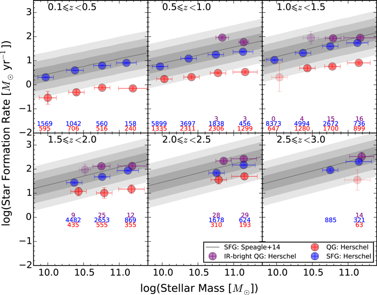
Figure 4. The SFR inferred from Herschel stacking as a function of M⋆ and z. The red (purple) circles represent the QG candidates below (above) the threshold of SFR24 = 100 M⊙ yr−1, and the blue circles represent the SFGs. The numbers at the bottom of each panel represent the median number of galaxies in each z and M⋆ bin for the Herschel stacking, and their colors follow the galaxy types specified in the legend. Note that these numbers are similar to, but not exactly the same as the numbers quoted on Tables 2–4 since we bootstrapped the Herschel stacking, as described in Section 3. The stacks with low S/N (fewer than two bands with S/N > 3) have larger error bars and are plotted in semi-transparent colors. The IR-bright QG candidates have similar or higher SFRH compared to SFGs, and are significantly higher than the IR-faint counterparts. For comparison, the SFR-M⋆ measured in Speagle et al. (2014) is plotted as gray lines, with the 1−3× observed dispersion (σSFR = 0.3) shown as dark-to-light shades. IR-faint QG candidates have SFRs at least 2–3 dispersions (0.6–0.9 dex) below those of SFGs out to z ∼ 2, and at z = 2–3 the difference is smaller.
Download figure:
Standard image High-resolution image
Figure 5. The SFR relative to SFRH as a function of M⋆ and z. The legend follows that of Figure 3. The error bars are derived from the propagation of the respective errors of SFRradio and SFRH.
Download figure:
Standard image High-resolution image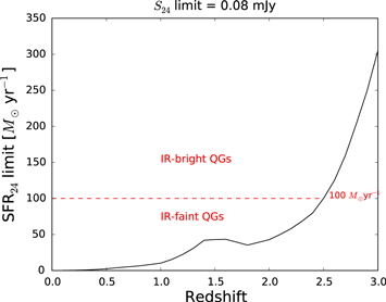
Figure 6. The 24 μm catalog is limited to sources brighter than 80 μJy (Le Floc'h et al. 2009; Lee et al. 2013). Applying the conversion of Rujopakarn et al. (2013) to convert S24 into SFR, we infer the corresponding SFR24 sensitivity limit as a function of redshift for the 24 μm catalog used in this work, shown as the black solid line. We separate QG candidates into "IR-bright" and "IR-faint" based on the SFR24 threshold of 100 M⊙ yr−1, as indicated by the red dashed line.
Download figure:
Standard image High-resolution imageAs a consistency check, we derive SFRs for SFG candidates from stacking MIR, FIR, and radio, using the same methods and assumptions stated above for QG candidates. The stacked fluxes are shown in the
4.5. Do IR-faint QGs Host AGNs?
By comparing the FIR-to-radio luminosity ratio of IR-faint QGs to that of SFGs, we can infer whether the radio emission, a tracer of total SF, is consistent with that expected for the amount of star formation observed at other wavelengths. Following the method described in Section 4.2, we use the FIR-radio correlation presented in Bell (2003) for SFGs and the dust SEDs fitted to the stacked Herschel fluxes to derive an expected radio synchrotron component (colored lines in Figure 2), which is then compared to the stacked 1.4 GHz fluxes (colored diamonds). We also plot SFRradio and compare them to SFRH on Figure 5. It is seen that the radio emissions of all galaxy types (SFGs, IR-faint, and IR-bright QGs) are in good agreement with the expectation from Herschel stacking, except for the most massive ( ) IR-faint QGs at z < 1.5 in which the radio emission is in excess, suggestive of radio emission originating from non-SF processes. The stacked radio flux densities do not vary beyond their stated uncertainties, if we include IR-bright QG candidates and/or exclude AGN hosts, since they comprise only a small fraction in each bin and we consider the median stacks (instead of mean).
We compute the logarithmic FIR-to-radio luminosity ratio as qIR = log( [W]/3.75 × 1012) − log(
 [W Hz−1]), where the
  used here refers to the Herschel-derived integrated IR luminosity over the rest-frame range of 8–1000 μm, and the
  refers to the rest-frame 1.4 GHz luminosity (see Section 4.2 for the derivation for both luminosities). The values of qIR are listed in Table 2. The radio luminosity
  [W Hz−1] increases with redshift from 1021.7 at z ∼ 0.4 to 1022.8 at z ∼ 1.2 for the most massive QGs, where the radio excess is the most prominent (see Figure 5). Beyond z ∼ 1.5, the radio stacks have S/N ≲ 5, therefore we are unable to quantify the radio excess at higher redshifts with certainty using the data at hand. Based on these results, we estimate that in the most massive QG candidates ∼60% of
  arises from non-SF processes. The radio excess may be even higher, and extend to higher z and lower M⋆, if old stellar populations account for significant Herschel emission of QGs (see Section 4.3).
Our results indicate that low-luminosity radio AGNs may be widespread among massive QGs, reciprocating the fact that massive QGs are the preferential hosts for low-luminosity radio AGNs (e.g., Smolčić et al. 2009; Baldi et al. 2014), and that radio-mode AGN feedback gains importance at later cosmic epochs at z < 1.5–2 (Croton et al. 2006). The fact that we only detect AGN contribution at radio wavelengths but not 24 μm in massive QGs is interesting for two reasons: (1) this is consistent with the expectation for luminous AGNs that selection criteria at different wavelengths have only slight overlaps, i.e., most AGNs identified at one wavelength do not fulfill the selection criteria at other wavelengths (e.g., Lemaux et al. 2014); (2) it indicates that only radio-mode feedback, but not (obscured) quasar-mode feedback, is at work in keeping the SF inefficient in massive QGs. However, it is not straightforward to use the median stacked radio luminosity to constrain the heating rate of radio-AGN feedback, without prior assumption of the duty cycle which is not well quantified.
We note that the radio excess for massive QGs at z < 1.5 are contingent on the validity of the assumptions used for converting stacked radio fluxes to SFRradio. This includes the assumption about the SED shapes for both the Herschel dust component, as well as the radio spectral slope for the FIR-radio correlation. There may also be systematic differences between the FIR-radio correlation by Bell (2003) used in this work compared to other works in literature (e.g., Ivison et al. 2010; Sargent et al. 2010; Magnelli et al. 2015), with regards to redshift evolution, luminosity evolution, primary sample selection, wavelength sampling of the dust peak and radio emission, etc. It is also unclear if the FIR-radio correlation calibrated for SFGs is applicable to QGs.
4.6. The Nature of IR-bright QG Candidates
Having separated the IR-bright QG candidates from the IR-faint ones in the stacking procedure, we list their stacked fluxes in Table 3 and plot their average SEDs in Figure 7 in the
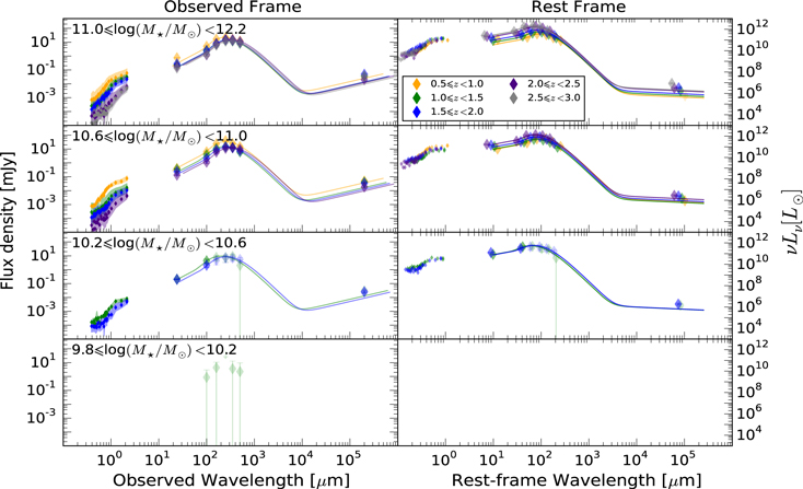
Figure 7. Panchromatic SEDs of IR-bright QG candidates with SFR yr−1. The legend follows that of Figure 2.
Download figure:
Standard image High-resolution image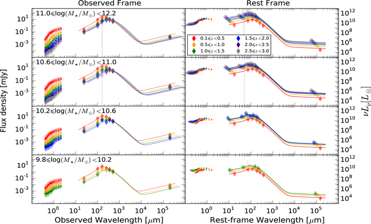
Figure 8. Panchromatic SEDs of SFG candidates. The legend follows that of Figure 2.
Download figure:
Standard image High-resolution imageCould the IR-bright QGs be the bright end of a unimodal log(LIR) distribution of all QGs? In  dex, compared to 0.2–0.3 dex for SFGs), if the IR-bright QGs belong to the bright tail of the log(LIR) distribution of QGs modeled by a Gaussian distribution.
4.7. Comparison with the Literature
Viero et al. (2013) and Schreiber et al. (2015) stacked Herschel maps for UVJ-selected galaxies. Viero et al. (2013) used the SIMSTACK code and found that massive ( ) QGs at z ∼ 2.3 (2.7) have
  . Schreiber et al. (2015) performed mean stacking with correction for the clustering bias, obtaining24
LIR ∼ 1011.4 L⊙ for QGs with M⋆ ∼ 1011.2 M⊙ at z ∼ 2.2. Our results in Section 4.4 indicate that z ≳ 2 IR-faint QGs have on average
. Schreiber et al. (2015) performed mean stacking with correction for the clustering bias, obtaining24
LIR ∼ 1011.4 L⊙ for QGs with M⋆ ∼ 1011.2 M⊙ at z ∼ 2.2. Our results in Section 4.4 indicate that z ≳ 2 IR-faint QGs have on average  . For a fair comparison to these works, we repeat our stacking procedures without separating IR-faint and IR-bright QG samples a priori based on their 24 μm emission, resulting in
  , which is similar to the average of the LIR of these two subsamples weighted by their numbers, i.e.,
  , where 1 and 2 represent IR-faint and IR-bright QGs, respectively. As QG candidates have higher 24 μm- and Herschel-bright fractions at z ≳ 2 (up to 15% and 6%, respectively, see Table 1 and Section 2), the inclusion of the quoted fractions of these IR-bright sources with LIR ∼ 1012.5L⊙ (see Table 3) boosts the stacked FIR emission of massive QGs at z ≳ 2 to be comparable to ULIRGs. These values are 0.1–0.3 dex lower than of those of Viero et al. (2013), which may be due to our inclusion of 24 μm sources not already selected in the UltraVISTA catalog (see Section 3) in the stacking procedure. Interestingly, the LIR estimates of Schreiber et al. (2015) are ∼0.6 dex lower than that of Viero et al. (2013), despite both stacking UVJ-selected QGs. The discrepancy is likely due to the different stacking algorithms used. Concluding this comparison, our Herschel stacking results are in broad agreement with those of Viero et al. (2013) and Schreiber et al. (2015). The variation of Herschel-derived LIR due to the different QG rest-frame color selections is negligible, when compared to the variation caused by different stacking algorithms.
Fumagalli et al. (2014) performed 24 μm stacking on 442 QGs at z = 0.3–2.5 with  , producing stacked flux densities of S24 ∼ 6−9 μJy, which are slightly lower than our results (see Table 2). Their sample is drawn from a smaller survey area equivalent to 11% of the UltraVISTA field, and therefore the discrepancy is likely explained by the fact that their sample is dominated by lower mass galaxies, which are more comparable to our stacked fluxes in lower stellar mass range (
 ). Qualitatively, we arrive at similar conclusions—QGs do not host strong obscured SF, and dust heating by evolved stellar populations may be significant at the low levels of LIR observed. The sSFR depression in QGs compared to SFGs may range from 2–10 in our work and in Schreiber et al. (2015), or 20–40 as claimed in Fumagalli et al. (2014), but the exact values depend on redshift and mass range, and are hard to quantify without further constraints on the relative contributions of the various dust heating mechanisms.
5. DISCUSSION AND SUMMARY
Our Herschel stacking results indicate that the NUVrJ selection successfully identify QGs over z = 0–3, with a maximum contamination fraction of 15% from dusty SFGs mostly at z ∼ 2–3, as estimated by cross-correlating to the 24 μm catalog with a sensitivity limit of 80 μJy. In other words, 24 μm fluxes are efficient for removing this small fraction of contaminants (IR-bright QG candidates) which host significant obscured SF. The IR-faint QGs have truly lower obscured SFRs compared to SFGs, as expected from their low unobscured SFRs measured from the UV continua. The average obscured sSFRs of IR-faint QGs with  are 5–13× lower than those of SFGs out to z = 2, based on Herschel stacking. At z = 2–3, the sSFRs of IR-faint QGs are only 2–5× below that of SFGs, suggesting that the classification between the two galaxy types may be less robust due to more uncertain rest-frame colors. For the most massive (
 ) IR-faint QGs at z = 0.1–1.5, the stacked radio emissions cannot be completely accounted for by the total level of SFRs derived from other indicators, suggesting the ubiquitous presence of low-luminosity AGNs at least out to z ∼ 1.5.
The  (and the resulting obscured SFR) derived from stacking 24 μm is a few factors lower than that derived from stacking Herschel for IR-faint QG candidates. This indicates that QGs have intrinsically different dust SED shape compared to SFGs, leading to an underestimation of the LIR from the stacked 24 μm flux. Alternatively, this suggests the presence of a cirrus dust component heated by old stellar populations in QGs. Spatially resolved FIR maps are needed to constrain the dust temperature gradient, and by comparing it to the distribution of old stars we can disentangle between these two scenarios. However, these resolved observations are currently only feasible for lensed galaxies. The James Webb Space Telescope will shed light on this matter in the near future.
We reaffirm that a population of truly quiescent galaxies is already in place by z = 3. This corroborates the need for powerful quenching mechanisms to terminate star formation in galaxies. While environmental quenching may be dominant for intermediate-mass QGs (Peng et al. 2010), stacking analyses at radio (this work) and X-ray (Olsen et al. 2013) wavelengths reveal that massive QGs harbor low-luminosity AGNs. AGNs provide a viable mechanism for quenching SF in galaxies, either through high-velocity outflows of gas (Tremonti et al. 2007; Cimatti et al. 2013; Cicone et al. 2014), or heating up the gas to prevent star formation. This is supported by the enhanced AGN fraction among transitory objects between SFGs and QGs (e.g., Barro et al. 2014). After galaxies are quenched, the AGNs may then proceed to "maintenance mode" suppressing further SF through a feedback cycle (Schawinski et al. 2009; Best & Heckman 2012). With upcoming surveys it will be possible to conduct a complete census of AGNs to sample the entire feedback duty cycle and constrain their energetics, in order to quantify their role in quenching star formation in galaxies.
We thank the COSMOS, UltraVISTA, PEP, and HerMES collaborations for providing the data used in this work. We are grateful to the anonymous referee for the invaluable comments that improved this manuscript. A.M. thanks Anna Gallazzi, Mark Sargent, Ryan Quadri, Brian Lemaux, and Julie Wardlow for helpful discussions. A.M. acknowledges the support of the Dark Cosmology Centre, which is funded by DNRF. T.R.G. acknowledges support from an STFC Advanced Fellowship. S.T. acknowledges support from the ERC Consolidator Grant funding scheme (project ConTExt, grant number 648179). A.K. acknowledges support by the Collaborative Research Council 956, sub-project A1, funded by the Deutsche Forschungsgemeinschaft (DFG). Support for B.M. was provided by the DFG priority program 1573 "The physics of the interstellar medium". C.M.C. acknowledges support from a McCue Fellowship through the University of California, Irvine's Center for Cosmology. V.S. is funded by the European Union's Seventh Frame-work program under grant agreement 337595 (ERC Starting Grant, "CoSMass"). A.Z. acknowledges support by the Instrument Centre for Danish Astrophysics (IDA). This work is based on data products from observations made with ESO Telescopes at the La Silla Paranal Observatory under ESO program ID 179.A-2005 and on data products produced by TERAPIX and the Cambridge Astronomy Survey Unit on behalf of the UltraVISTA consortium.
APPENDIX: ARE THE IR-BRIGHT QG CANDIDATES THE TAIL OF THE ENTIRE DISTRIBUTION?
Are the IR-bright QGs merely the high-end tail of a broad unimodal distribution, or are they in fact misclassifications (i.e., the log(LIR) is a bimodal distribution)?
Bimodal distributions are usually defined to have significant separation between the two means compared to the combined dispersions. The lack of individual IR detections for all QG candidates hinders us from deriving the underlying distributions and dispersions, therefore we are unable to answer this question directly. However, if their log(LIR) distribution are unimodal, we can constrain the dispersion required to reproduce the population mean, as well as the mean of the bright subset, given the number of QGs and IR-bright QGs in each z and M⋆ bin. Assuming the log(LIR) distribution is Gaussian, the dispersion can be calculated as:
where erfcinv(x) ≡ erfc−1(x) is the inverse complementary error function of x.
Based on the LIR,H and NQG on Tables 2 and 3, we calculate the expected  and list them on Table 5. They are larger than the 0.3 dex of dispersion measured for SFGs (Speagle et al. 2014). While these numbers cannot be used to infer the intrinsic log(LIR) distribution of QG candidates, we conclude that a broad distribution is required if the IR-bright QG canadidates are the brightest subset of all QG candidates. In another words, we rule out the possibility of a narrow (
 ), unimodal Gaussian distribution of log(LIR) of QG candidates.
Table 5. Expected Dispersion of log(LIR) for QG Candidates
| log(M⋆/M⊙) | ||||
|---|---|---|---|---|
| Redshift | 11–12.2 | 10.6–11 | 10.2–10.6 | 9.8–10.2 |
| 0.1–0.5 | ⋯ | ⋯ | ⋯ | ⋯ |
| 0.5–1.0 | 0.40 | 0.45 | ⋯ | ⋯ |
| 1.0–1.5 | 0.42 | 0.43 | 0.42 | ⋯ |
| 1.5–2.0 | 0.41 | 0.47 | 0.37 | ⋯ |
| 2.0–2.5 | 0.37 | 0.37 | ⋯ | ⋯ |
| 2.5–3.0 | 0.46 | ⋯ | ⋯ | ⋯ |
Note. The expected dispersion of log(LIR) for NUVrJ-selected QG candidates, if the log(LIR) is approximated as a unimodal Gaussian distribution.
Download table as: ASCIITypeset image
Footnotes
- 13
Herschel is an ESA space observatory with science instruments provided by European-led Principal Investigator consortia and with important participation from NASA.
- 14
SPIRE has been developed by a consortium of institutes led by Cardiff Univ. (UK) and including: Univ. Lethbridge (Canada); NAOC (China); CEA, LAM (France); IFSI, Univ. Padua (Italy); IAC (Spain); Stockholm Observatory (Sweden); Imperial College London, RAL, UCL-MSSL, UKATC, Univ. Sussex (UK); and Caltech, JPL, NHSC, Univ. Colorado (USA). This development has been supported by national funding agencies: CSA (Canada); NAOC (China); CEA, CNES, CNRS (France); ASI (Italy); MCINN (Spain); SNSB (Sweden); STFC, UKSA (UK); and NASA (USA).
- 15
We refer to them as "candidates" since their galaxy types are not spectroscopically confirmed.
- 16
Including the incomplete bins in the Herschel stacking does not change the stacked flux densities by more than their quoted uncertainties.
- 17
The sensitivity limit of the Spitzer 24 μm map implies that only SFR24 > 43 (305) M⊙ yr−1 at z = 2 (3) will be detected, as shown in Figure 6. Therefore we may not be complete in identifying QG candidates with SFR24 = 100–305 M⊙ yr−1 at z = 2.5–3, thus partially accounting for the higher sSFR at z ≳ 2 detailed in Section 4.4.
- 18
- 19
Decimal exponent, i.e., x dex = 10x.
- 20
- 21
SFR
= SFR. - 22
- 23
- 24


